Next Article in Journal
PRGF-Modified Collagen Membranes for Guided Bone Regeneration: Spectroscopic, Microscopic and Nano-Mechanical Investigations
Next Article in Special Issue
Loop Closure Detection Based on Multi-Scale Deep Feature Fusion
Previous Article in Journal
Effect of Carbon Nanotubes on Chloride Penetration in Cement Mortars
Previous Article in Special Issue
Multi-Robot Trajectory Planning and Position/Force Coordination Control in Complex Welding Tasks
 
 
Correction published on 29 May 2019, see Appl. Sci. 2019, 9(11), 2215.
Article

Biologically-Inspired Learning and Adaptation of Self-Evolving Control for Networked Mobile Robots

1
Graduate Institute of Automation and Control, National Taiwan University of Science and Technology, Taipei City 10607, Taiwan
2
Department of Electrical Engineering, National Ilan University, Yilan City 26047, Taiwan
*
Author to whom correspondence should be addressed.
Appl. Sci. 2019, 9(5), 1034; https://doi.org/10.3390/app9051034
Submission received: 16 January 2019 / Revised: 26 February 2019 / Accepted: 5 March 2019 / Published: 12 March 2019
(This article belongs to the Special Issue Advanced Mobile Robotics)

Abstract

:
This paper presents a biologically-inspired learning and adaptation method for self-evolving control of networked mobile robots. A Kalman filter (KF) algorithm is employed to develop a self-learning RBFNN (Radial Basis Function Neural Network), called the KF-RBFNN. The structure of the KF-RBFNN is optimally initialized by means of a modified genetic algorithm (GA) in which a Lévy flight strategy is applied. By using the derived mathematical kinematic model of the mobile robots, the proposed GA-KF-RBFNN is utilized to design a self-evolving motion control law. The control parameters of the mobile robots are self-learned and adapted via the proposed GA-KF-RBFNN. This approach is extended to address the formation control problem of networked mobile robots by using a broadcast leader-follower control strategy. The proposed pragmatic approach circumvents the communication delay problem found in traditional networked mobile robot systems where consensus graph theory and directed topology are applied. The simulation results and numerical analysis are provided to demonstrate the merits and effectiveness of the developed GA-KF-RBFNN to achieve self-evolving formation control of networked mobile robots.

1. Introduction

Networked mobile robots that are capable of self-learning have received growing attention in the mobile robotics research community [1,2,3]. This emerging technology has surpassed the conventional robotic system by taking advantage of robot collaboration, system robustness, scalability, and greater flexibility. This modern robotic system has been commonly applied in manufacturing, military applications, surveillance, etc. to perform complex tasks [4,5,6]. Some self-learning strategies have been proposed to develop motion controllers for networked mobile robots [6,7]. Among them, an RBFNN incorporating the gradient descent method is regarded as a powerful tool for designing the self-learning controllers of networked mobile robots [7,8].
The RBFNN introduced by Broomhead and Lowe is a three-layer feedforward artificial neural network in which radial basis functions are used as activation functions [9,10]. This methodology takes advantage of fast learning capability and universal approximation. To date, it is a useful neural network architecture for addressing many engineering problems [11,12]. However, traditional RBFNNs adopt a gradient descent approach for training the neural network that is not capable of noise reduction [10,11,12]. In other words, these studies did not consider the uncertainty and noise induced in the process and measurement phases. This paper presents a Kalman filter based RBFNN and its application to self-learning control of networked mobile robots.
The Kalman filter is a state estimation technique introduced by R.E. Kalman [13]. It is a classic state estimation technique used widely in engineering applications, including spacecraft navigation, motion planning in robotics, signal processing and wireless sensor networks [14,15,16] because of its ability to extract useful information from noisy data. It is an optimal estimator for evaluating the internal state of a dynamic system under certain process patterns and/or measurement disturbances in the physical environment [13,17,18]. The objective of the Kalman filter is to minimize the mean squared error between the actual and estimated data. Although the proposed KF-RBFNN is useful for designing learning control schemes with noise reduction, the initial network parameters influences the system performance, namely that the selection of centers, widths and output weights for the Gaussian functions is an important consideration.
Parameter-tuning of an RBFNN is challenging when using this neural network to solve multidimensional optimization problems. Over the years, several methods have been developed for addressing this RBFNN optimization problem [19,20,21]. However, these traditional RBFNN methods may cause the output to converge to local optimum when the dimensionality of the problem increases [22]. Since RBFNN optimization can be formulated as a search problem, biologically, algorithms are new paths for optimizing RBFNNs. This is a successful hybridization of RBFNNs and evolutionary algorithms. Although there are some metaheuristic algorithms used to develop evolutionary RBFNNs [23,24,25,26], there has been no attempt to present an evolutionary KF-RBFNN using a GA to achieve learning control of networked mobile robotic systems.
The GA is one of the most popular evolutionary algorithms for solving optimization problems [27,28,29]. Although GAs have been widely applied to various optimization problems, these biologically inspired algorithms suffer from premature convergence. In other words, these traditional computing paradigms may converge to local optimum. This paper contributes to the development of a modified GA to improve the search diversity by including the Lévy flight approach. An adaptive determination of crossover and mutation probabilities in the GA is proposed via the Lévy flights. This random walk is very efficient in exploring the search space of the optimization problem. The proposed modified GA metaheuristics is then applied to the design of an optimal GA-KF-RBFNN for self-tuning motion control of networked mobile robots.
Of the increasing demands on networked mobile robot systems, formation using a leader-follower control strategy is one of the most important and is becoming increasing crucial [30,31,32]. It is a coordinated control in which the leader robot follows a desired trajectory while the follower robots maintain a specified geometrical pattern [32]. Although some studies have addressed this control problem by considering graph theory and consensus control approaches [33,34,35], these networked mobile robot systems suffer from communication delay problem. This paper presents a pragmatic self-learning optimal GA-KF-RBFNN formation control method for networked mobile robot systems that avoids the communication delay problem.
This paper is structured as follows: a biologically-inspired Kalman filter based RBFNN control technique, called GA-FA-RBFNN control is introduced in Section 2. Section 3 employs the proposed GA-FA-RBFNN to develop a networked mobile robot system to achieve self-evolving formation control. In Section 4, several simulation results are reported to demonstrate the effectiveness of the proposed methods. Finally, Section 5 concludes this paper.

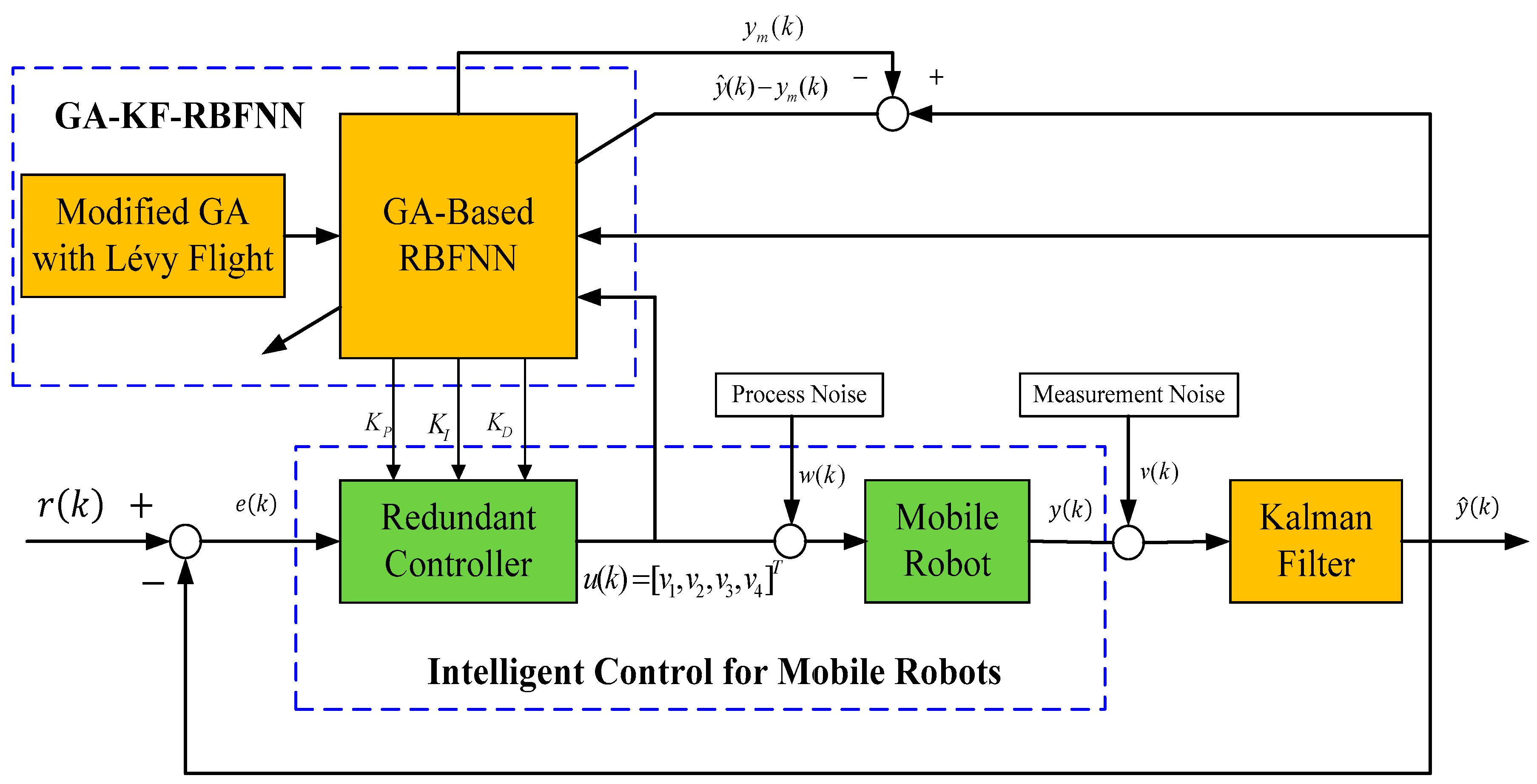
2. Biologically-Inspired Kalman Filter Based RBFNN Control

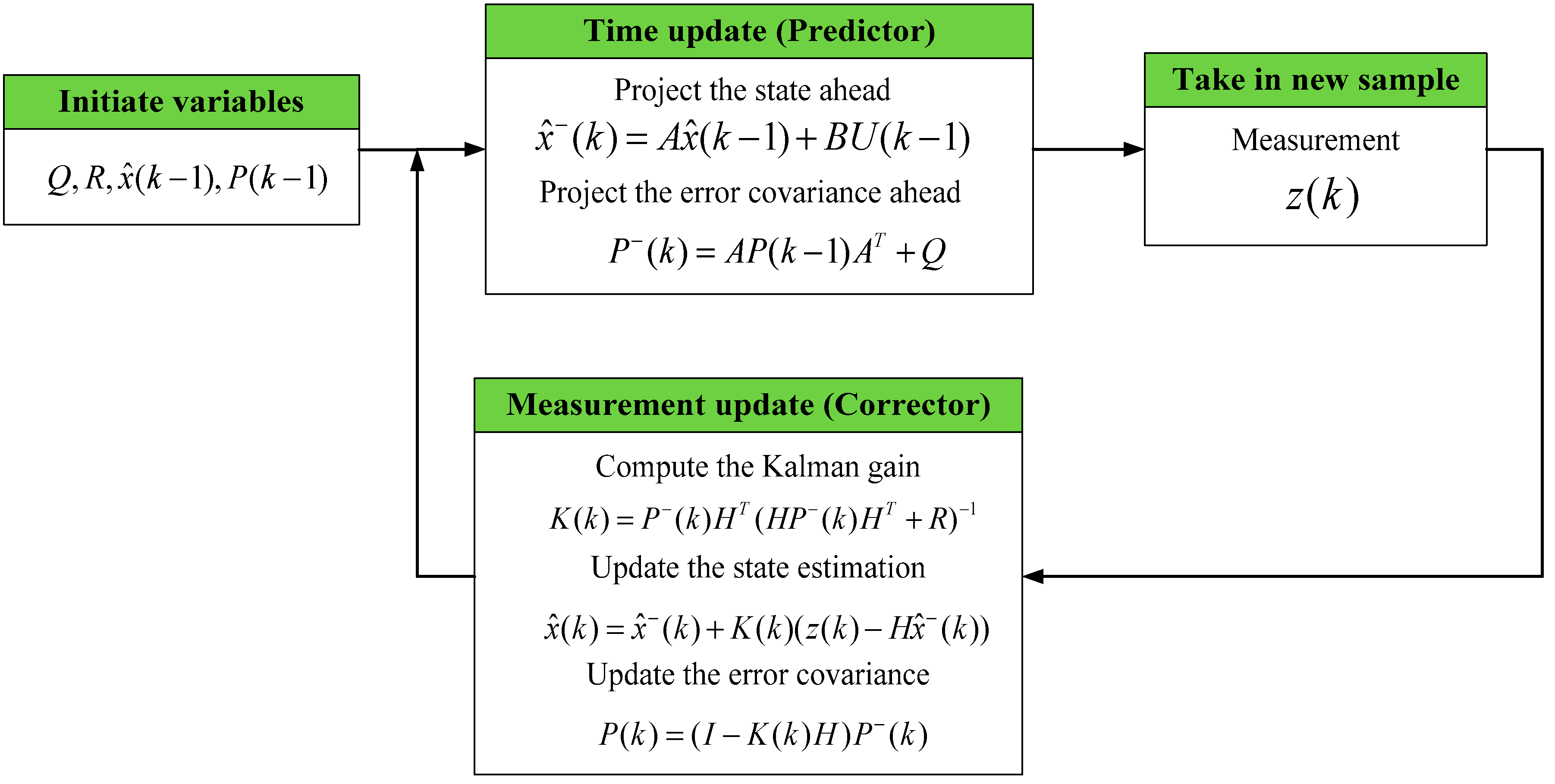
2.1. Kalman Filter Algorithm

This section aims to describe the Kalman filter algorithm by which measurements are taken, and the state is estimated at discrete time points. The Kalman filter deals with the general problems encountered in estimating the state of a discrete-time controlled process, which is governed by the following state-space Equation (1) at time index k:
x ( k ) = A x ( k 1 ) + B U ( k 1 ) + w ( k ) y ( k ) = C x ( k ) z ( k ) = H y ( k ) + v ( k )
where A, B, and C are matrices in the state-space Equation (2). w ( k ) is the process noise and v ( k ) is the measurement noise. z ( k ) is the measured signal and H is the sensor matrix. The probability of the process noise w ( k ) is p(w) and the probability of measurement noise v ( k ) is p(v). The process noise covariance of p(w) is Q and the measured noise covariance of p(v) is R. In Kalman filtering, p(w) and p(v) are independent white noises with normal probability distributions, expressed by:
p ( w ) N ( 0 , Q ) p ( v ) N ( 0 , R )
Figure 1 presents the structure of Kalman filter algorithm in which the estimated state x ^ ( k 1 ) and the error covariance P(k − 1) are included [13]. As shown in Figure 1, The Kalman filter algorithm consists of two phases: time update phase (predictor) and measurement update phase (corrector). The following summarizes the two important phases in classical Kalman filter algorithm.
  • Time update phase:
    • At time step k − 1, calculate x ^ ( k 1 ) and P ( k 1 ) .
    • Update the estimation of state vector x ^ ( k ) and the estimation of error covariance matrix P ^ ( k ) .
  • Measurement update phase:
    • Update the optimal gain K(k) of Kalman filter.
    • Update the estimation of state vector x ^ ( k ) using z ( k ) , x ^ ( k ) and K(k).
    • Update the estimation of error covariance matrix p(k) by utilizing K(k) and P ( k ) for next iteration in the Kalman filter algorithm process.

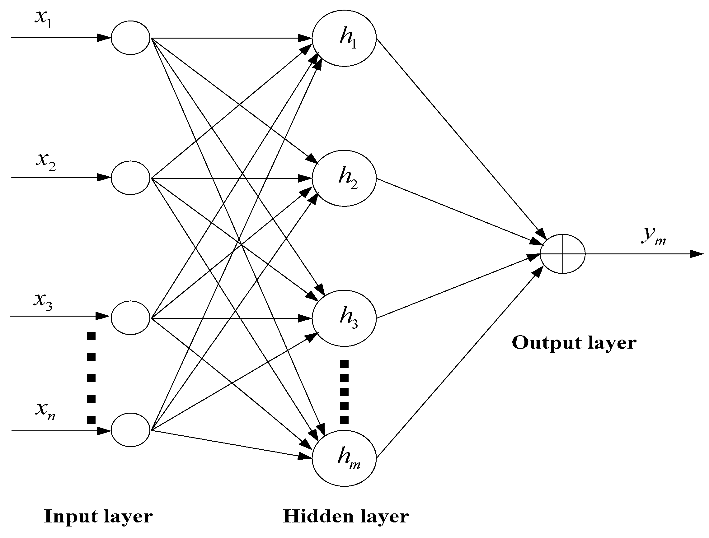
2.2. Classical RBFNN

Figure 2 presents the structure of a classical RBFNN. This feed forward multilayer neural network has three layers, comprising the input layer, hidden layer and output layer. As shown in Figure 2, the inputs of the hidden layer in the RBFNN structure are the linear combinations of the weights and the input vector [ x 1   x 2 ,   x 3 ,   ,   x n ] T . These vectors are then mapped by means of a radial basis functions in each node. Finally, the output layer of RBFNN generates a vector y p for m outputs by linear combination of the outputs of the hidden nodes. This kind of artificial neural network has been regarded as a powerful tool that can approximate any continuous function with satisfactory accuracy [11]. In Figure 2, the output of the RBFNN is expressed by:
y m = j = 1 m w j h j
where h j is the radial basis vector. This vector is described by using the following Gaussian function:
h j = exp ( X C j 2 2 b j 2 ) , j = 1 , 2 , , m
where is the Euclidean norm operation, C j = [ c j 1 , c j 2 ,   ,   c j m ] T is the center vector of the jth node, B = [ b 1 , b 2 ,   ,   b m ] T is the basis width vector. W = [ w 1 , w 2 ,   ,   w m ] T is the weight vector in the RBFNN. Typically, this neural network is initialized with a randomly determined of RBFNN parameters, including C j , B , and W .
Gradient descent is an effective method for training RBFNN networks compared with other conventional training approaches [9,10]. In gradient descent training with one neuron in the output layer, the weights are updated at each time step by using the following rules:
w j ( k + 1 ) = w j ( k ) + η e ( k ) h j ( k ) ,
C j i ( k + 1 ) = C j i ( k ) + η e ( k ) w j h j x i ( k ) C j i ( k ) b j 2 ( k ) ,
b j ( k + 1 ) = b j ( k ) + η e ( k ) w j h j X ( k ) C j ( k ) 2 b j 3 ( k ) ,
where e ( k ) represents the error at the kth time step and η denotes the learning rate. Since the initial parameters for an RBFNN using the gradient descent method are determined either by a trial-and-error approach or randomly set, convergence to a local optimum solution is inevitable [10]. To improve the learning performance of the RBFNN, this paper has developed a Kalman filter to train the RBFNN network structure based on a gradient descent approach. The proposed KF-RBFNN is applied to the self-learning control of networked mobile robots.

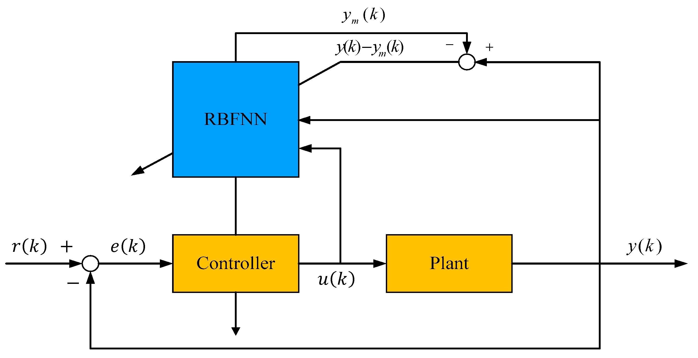
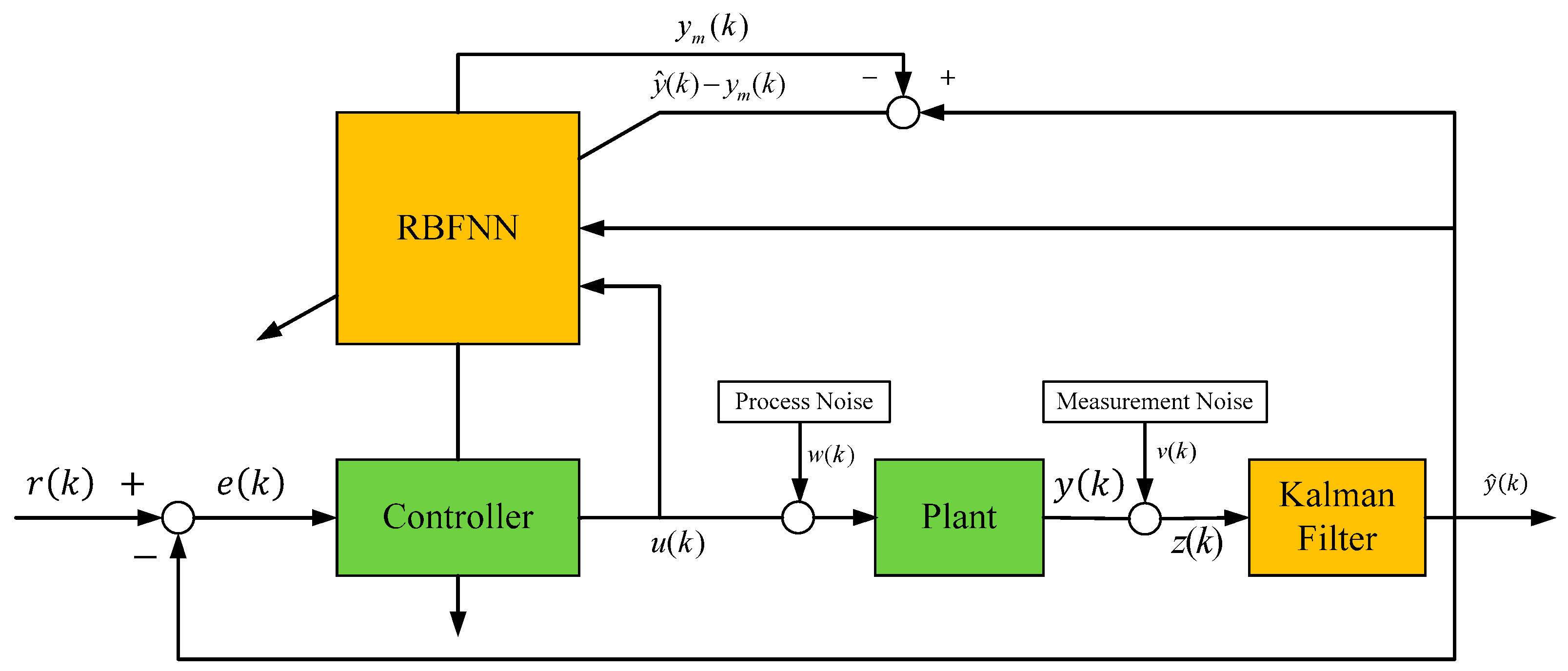
2.3. Kalman Filter Based RBFNN Control

Figure 3 depicts the block diagram of the RBFNN-based control. In Figure 3, the error between the real output y(k) and the estimated output of the neural network y m ( k ) are considered to develop a self-learning RBFNN. The cost function or performance index is defined by the squared estimation error:
J ( k ) = 1 2 [ y ( k ) y m ( k ) ] 2 .
Considering the gradient descent method in Equations (5)–(7), the structure parameters: wj, Cji, and bj are updated online at every sampling point, expressed by:
Δ w j = [ y ( k ) y m ( k ) ] h j w j ( k ) = w j ( k 1 ) + η Δ w j + ς [ w j ( k 1 ) w j ( k 2 ) ] Δ b j = [ y ( k ) y m ( k ) ] w j h j X C j 2 b j 3 b j ( k ) = b j ( k 1 ) + η Δ b j + ς [ b j ( k 1 ) b j ( k 2 ) ] Δ c j i = [ y ( k ) y m ( k ) ] w j x j c j i b j 2 c j i ( k ) = c j i ( k 1 ) + η Δ c j i + ς [ c j i ( k 1 ) c j i ( k 2 ) ] ,
where ς denotes the momentum factor and η is the learning rate of the neural network.
Based on Figure 3, the proposed KF-RBFNN control scheme depicted in Figure 4 considers the process noise w(k) and measurement noise v(k). In the proposed intelligent KF-RBFNN control scheme, the KF-RBFNN serves as an on-line learning and adapting mechanism in the intelligent controller. As shown in Figure 4, the effects of the process uncertainty w(k) and the measurement noise v(k) in the control scheme can be reduced via the implementation of the Kalman filter. To retrain the uncertainty and noise, the measured output z(k) is employed to derive an estimation y ^ ( k ) of the output y(k) in the proposed KF-RBFNN. Both the control signal u(k) and output y m ( k ) of the RBFNN are fed into the neural network for on-line learning. Moreover, the estimated output value y m ( k ) of the RBFNN is then utilized to update the control parameters to achieve self-learning control using the Kalman filter.

2.4. Evolutionary KF-RBFNN Control

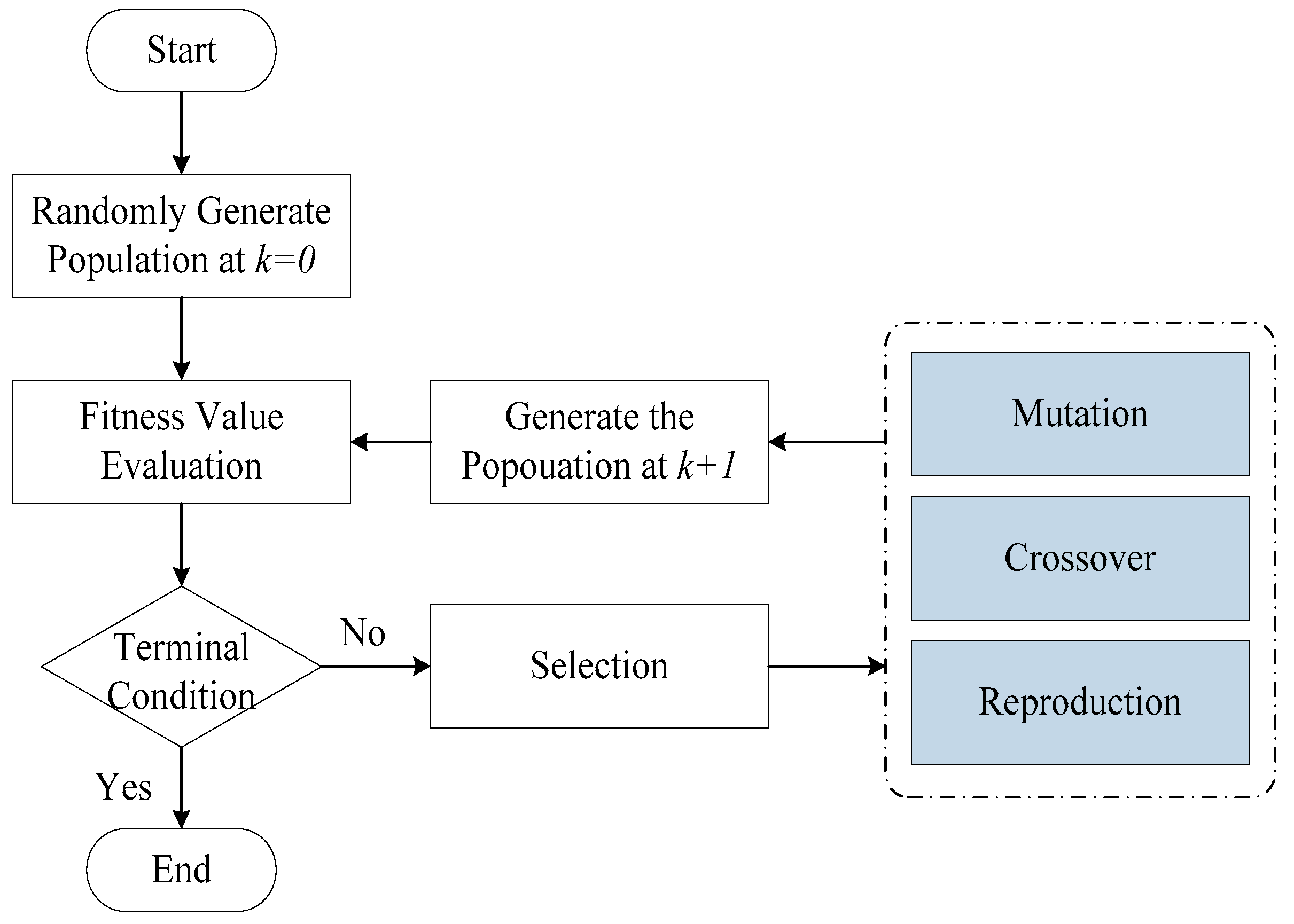
2.4.1. Modified GA with Lévy Flight

The GA developed by John Holland is a search algorithm that is inspired by Charles Darwin’s theory of natural evolution. This evolutionary algorithm reflects the process of natural selection where the fittest individuals are selected for reproduction, thereby producing offspring of the next generation. This stochastic optimization technique starts with a set of solutions (chromosomes), called a population. This paradigm employs probabilistic rules to evolve a population from one generation to the next via the genetic operators: reproduction, crossover, and mutation. This paradigm is widely used to solve multidimensional optimization problems. When applying a GA to deal with optimization problems, an initial population of feasible solutions is generated. Each feasible solution is encoded as a chromosome string. These chromosomes are evaluated using a predefined fitness function or objective function based on the optimization problems. Figure 5 presents the flowchart of a GA. The initial population is randomly generated and the fitness function is defined before the GA evolutionary process begins. This study employs tournament selection, single-point crossover and single-point mutation strategies to develop a modified GA paradigm.
Crossover and mutation are important operations for generating new individuals in the GAs. The performance of a GA is sensitive to the control parameter setting. The probabilities of crossover and mutation are significant parameters that influence the convergence performance of a GA. The use of unsuitable probability for crossover and mutation can result in poor convergence performance. More precisely, choosing suitable parameter values is a problem dependent task and requires previous experiences. Most studies adopt fixed crossover and mutation probabilities; this paper employs the Lévy flight which is a specialized random walk to increase the search diversity, expressed by:
L e v y ( β ) = | Γ ( β + 1 ) × sin ( π β 2 ) Γ ( 1 + β 2 ) × β × 2 ( β 1 2 ) | 1 β ,
where Γ denotes the gamma function and β is a constant ( 1 < β 3 ) . The proposed modified GA is then applied to optimally set the initial parameters of the KF-RBFNN.

2.4.2. GA-Based KF-RBFNN

In the proposed KF-RBFNN, the accuracy and performance are influenced by the selections of the radial functions that are defined by a center vector B, width vector Cj, and weight vector W. In other words, proper tuning of these parameters is an important part of the optimal KF-RBFNN designs. This study employs the modified GA to develop a parameter tuning process that optimizes the KF-RBFNN. When applying the GA to address this issue, a chromosome is defined by the RBFNN parameter sequence C h r o m o s o m e = { C j , B , W } and the optimal RBFNN structure can be evolved via the GA process with Lévy flight. The following fitness function (root mean square error, RMSE) for the N s sample is used to evaluate the GA chromosomes.
F i t n e s s = 1 N s k = 1 N s ( y p * ( k ) y p ( k ) ) 2
where y p ( k ) is the output and y p * ( k ) is the predicted output at the kth sampling time. The following describes the GA process for KF-RBFNN optimization.
Step 1:
Initialize the GA computing with Lévy flight.
Step 2:
Each GA chromosome in the population contains genes to represent the KF-RBFNN parameters, meaning that C h r o m o s o m e = { C j , B , W } .
Step 3:
Construct the KF-RBFNN using C h r o m o s o m e = { C j , B , W } and evaluate the performance using the fitness function (11).
Step 4:
Perform GA crossover and mutation with the probabilities set by Lévy flight.
Step 5:
Update the GA population.
Step 6:
Check the termination criterion. Go to Step 3 or output the optimized GA individual C h r o m o s o m e * = { C j * , B * , W * } for the proposed GA-KF-RBFNN.

3. Application to Self-Evolving Control of Networked Mobile Robots

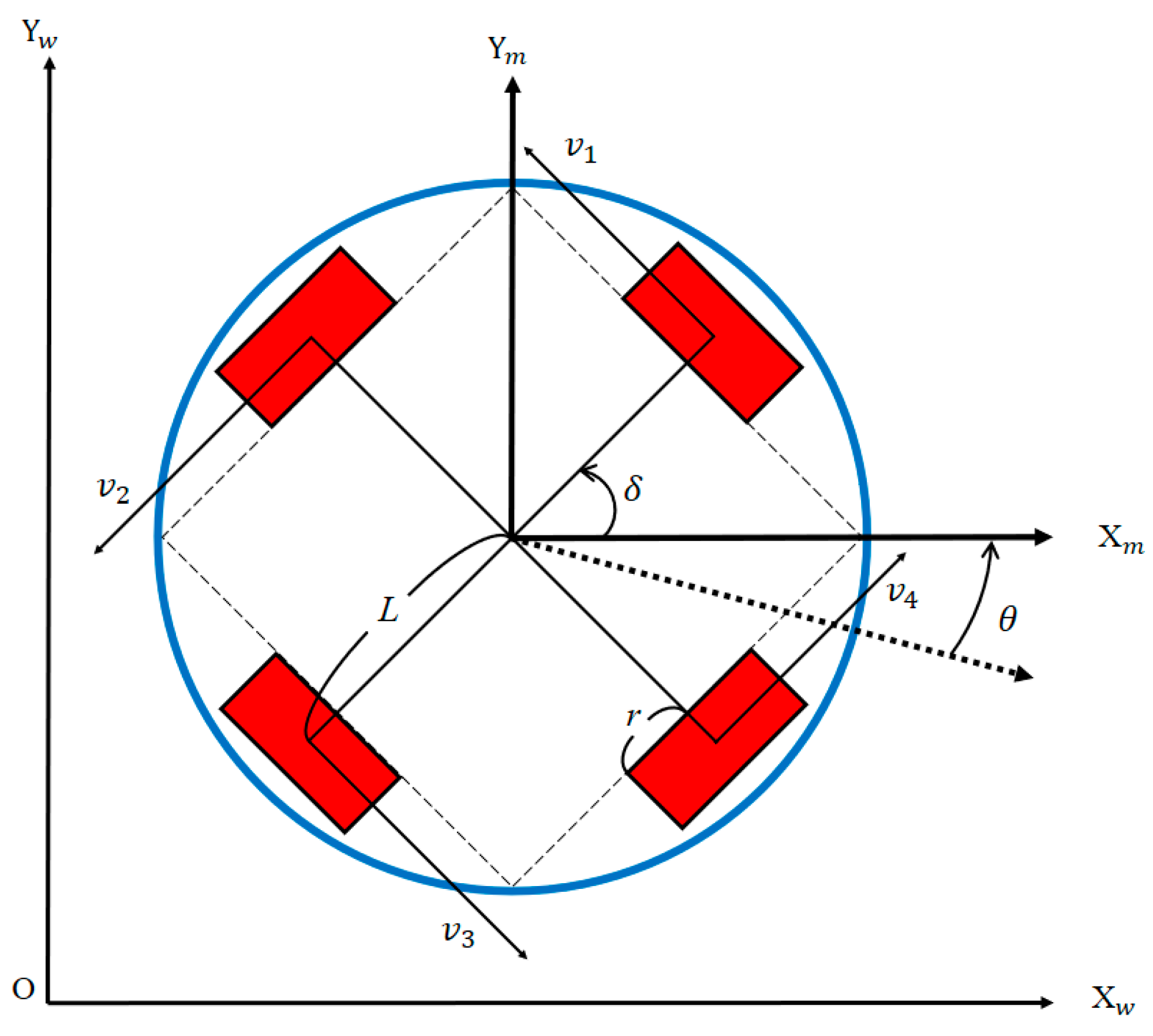
3.1. Modeling and Lyapunov-Based Control

Figure 6 depicts the geometrical structure of a mobile robot with four Swedish wheels for the proposed networked mobile robot system. Compared to the conventional differential-drive (non-holonomic) mobile robots, this kind of mobile robot with omnidirectional capability has superior mobility. The kinematic model of the four-wheeled Swedish mobile robot is expressed by:
[ v 1 ( t ) v 2 ( t ) v 3 ( t ) v 4 ( t ) ] = [ r ω 1 ( t ) r ω 2 ( t ) r ω 3 ( t ) r ω 4 ( t ) ] = T ( θ ( t ) ) [ x ˙ ( t ) y ˙ ( t ) θ ˙ ( t ) ] ,
where:
T ( θ ( t ) ) = [ sin ( δ + θ ) cos ( δ + θ ) sin ( δ + θ ) cos ( δ + θ ) cos ( δ + θ ) sin ( δ + θ ) cos ( δ + θ ) sin ( δ + θ ) L L L L ] ,
δ is π / 4 ; r represents the radius of the Swedish wheel; L denotes the distance from the Swedish wheel’s center to the geometric center of the mobile robot; v i ( t ) and ω i ( t ) , i = 1 , 2 , 3 , 4 respectively denote the linear and angular velocities of each omnidirectional wheel. [ x ( t )   y ( t )   θ ( t ) ] T is the pose vector that includes the position and orientation of the mobile robot measured at time t.
In mobile robotic research, robots with over three degrees-of-freedom (DOFs) are classified as redundant robots because they provide redundancy. Note that T ( θ ( t ) ) in Equation (12) is singular for any θ in this redundant mobile robot system. This study adopts the pseudo inverse matrix approach to address the redundant control problem of mobile robots. Considering the left pseudo-inverse matrix T # ( θ ( t ) ) of T ( θ ( t ) ) by using T # ( θ ( t ) ) P ( θ ( t ) ) = I , the matrix T # ( θ ( t ) ) is expressed by:
T # ( θ ( t ) ) = [ sin ( δ + θ ) 2 cos ( δ + θ ) 2 1 4 L cos ( δ + θ ) 2 sin ( δ + θ ) 2 1 4 L sin ( δ + θ ) 2 cos ( δ + θ ) 2 1 4 L cos ( δ + θ ) 2 sin ( δ + θ ) 2 1 4 L ] .
Combining Equations (12) and (13), the kinematics of the four-wheeled omnidirectional mobile robot is derived as follows:
[ x ˙ ( t ) y ˙ ( t ) θ ˙ ( t ) ] = T # ( θ ( t ) ) [ v 1 ( t ) v 2 ( t ) v 3 ( t ) v 4 ( t ) ] .
After the kinematics analysis of the Swedish mobile robots, the next step is to design a motion control law and prove its stability using Lyapunov theory. The current pose of the omnidirectional Swedish mobile robot at time t is defined as S = [ x ( t ) y ( t ) θ ( t ) ] T , and the desired reference trajectory of the Swedish mobile robot is expressed as S r = [ x r ( t ) y r ( t ) θ r ( t ) ] T . With the two pre-defined vectors, the tracking error of the mobile robot is given by:
S e = [ x e ( t ) y e ( t ) θ e ( t ) ] = [ x ( t ) y ( t ) θ ( t ) ] [ x r ( t ) y r ( t ) θ r ( t ) ] = S S r ,
which gives:
S ˙ e = [ x ˙ e ( t ) y ˙ e ( t ) θ ˙ e ( t ) ] = [ x ˙ ( t ) y ˙ ( t ) θ ˙ ( t ) ] [ x ˙ r ( t ) y ˙ r ( t ) θ ˙ r ( t ) ] = T # ( θ ( t ) ) [ r ω 1 ( t ) r ω 2 ( t ) r ω 3 ( t ) r ω 4 ( t ) ] [ x ˙ r ( t ) y ˙ r ( t ) θ ˙ r ( t ) ] .
The goal of control law design is to derive the angular velocity vector [ ω 1 ( t ) ω 2 ( t ) ω 3 ( t ) ω 4 ( t ) ] T for tracking the desired differentiable trajectory [ x r ( t ) y r ( t ) θ r ( t ) ] T with asymptotical stability. Based on the PID (Proportional-Integral-Derivative) control strategy, the following redundant control law is proposed:
[ v 1 ( t ) v 2 ( t ) v 3 ( t ) v 4 ( t ) ] = T ( θ ( t ) ) ( K P [ x e ( t ) y e ( t ) θ e ( t ) ] K I [ 0 t x e ( τ ) d τ 0 t y e ( τ ) d τ 0 t θ e ( τ ) d τ ] K D [ x ˙ e ( t ) y ˙ e ( t ) θ ˙ e ( t ) ] + [ x ˙ r ( t ) y ˙ r ( t ) θ ˙ r ( t ) ] ) ,
where K P , K I   and   K D are the control matrices. They are diagonal and positive, thus K P = d i a g [ k x p   k y p   k θ p ] , K I = d i a g [ k x i   k y i   k θ i ] , and K D = d i a g [ k x d   k y d   k θ d ] . By substituting Equations (17) into (16), the closed-loop error system is obtained:
S ˙ e = [ x ˙ e ( t ) y ˙ e ( t ) θ ˙ e ( t ) ] = ( K P [ x e ( t ) y e ( t ) θ e ( t ) ] K I [ 0 t x e ( τ ) d τ 0 t y e ( τ ) d τ 0 t θ e ( τ ) d τ ] K D [ x ˙ e ( t ) y ˙ e ( t ) θ ˙ e ( t ) ] ) .
To prove the asymptotical stability of the closed-loop error system in (18) via Lyapunov theory, the following Lyapunov function is selected:
V ( t ) = 1 2 [ x e ( t ) y e ( t ) θ e ( t ) ] [ x e ( t ) y e ( t ) θ e ( t ) ] + 1 2 [ 0 t x e ( τ ) d τ 0 t y e ( τ ) d τ 0 t θ e ( τ ) d τ ] K I [ 0 t x e ( τ ) d τ 0 t y e ( τ ) d τ 0 t θ e ( τ ) d τ ] + 1 2 [ x e ( t ) y e ( t ) θ e ( t ) ] K D [ x e ( t ) y e ( t ) θ e ( t ) ] > 0
one obtains:
V ˙ ( t ) = [ x e ( t ) y e ( t ) θ e ( t ) ] K P [ x e ( t ) y e ( t ) θ e ( t ) ] < 0 .
Since V ˙ is negative definite, the asymptotical stability is therefore proven. The proposed motion control law can steer the mobile robot to achieve S S r as t .

3.2. GA-KF-RBFNN Self-Learning Control

Figure 7 depicts the GA-KF-RBFNN self-learning control scheme, in which the noise from the process and measurement phases are included. As shown in Figure 7, the proposed GA-KF-RBFNN is employed to online adjust the parameters K P = d i a g [ k x p   k y p   k θ p ] , K I = d i a g [ k x i   k y i   k θ i ] , and K D = d i a g [ k x d   k y d   k θ d ] of the mobile robot. It is worthy to mention that the control matrices in Equation (17) are online adjusted at every sampling point to achieve tracking control. This GA-KF-RBFNN evolutionary online tuning method with noise reduction outperforms the traditional off-line and hand-tuning approaches.
In Figure 7, the control law u ( k ) = [ v 1 , v 2 , v 3 , v 4 ] T and the output y m ( k ) of the RBFNN are fed into the network for on-line learning. Moreover, the estimated output value y m ( k ) of the RBFNN is then employed to update the control matrices K P = d i a g [ k x p   k y p   k θ p ] , K I = d i a g [ k x i   k y i   k θ i ] , and K D = d i a g [ k x d   k y d   k θ d ] of the four-wheeled omnidirectional mobile robot to achieve the auto-tuning control with a Kalman filter.

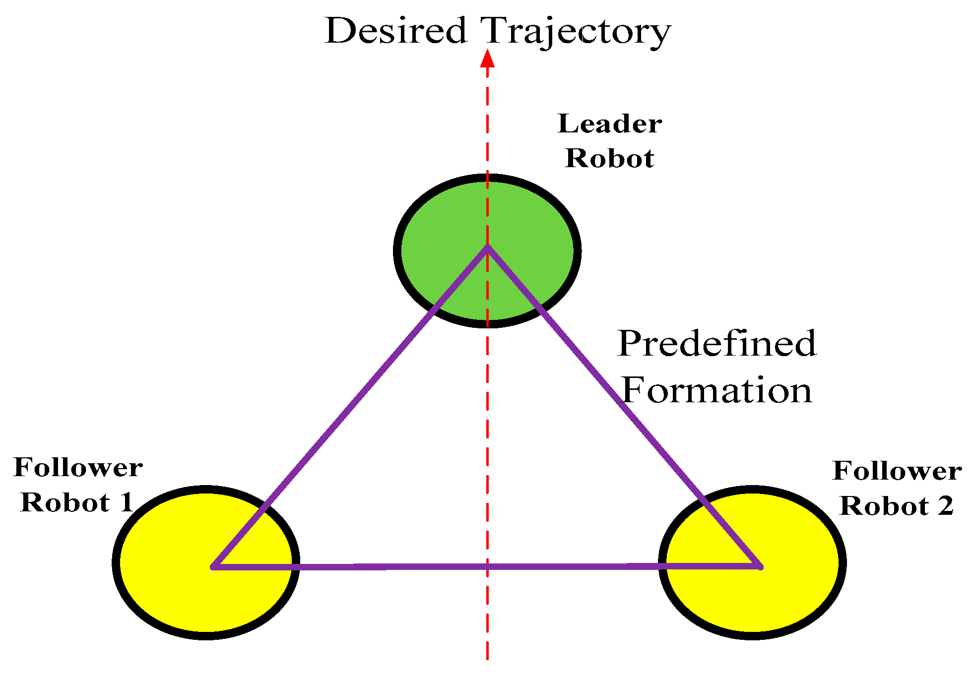
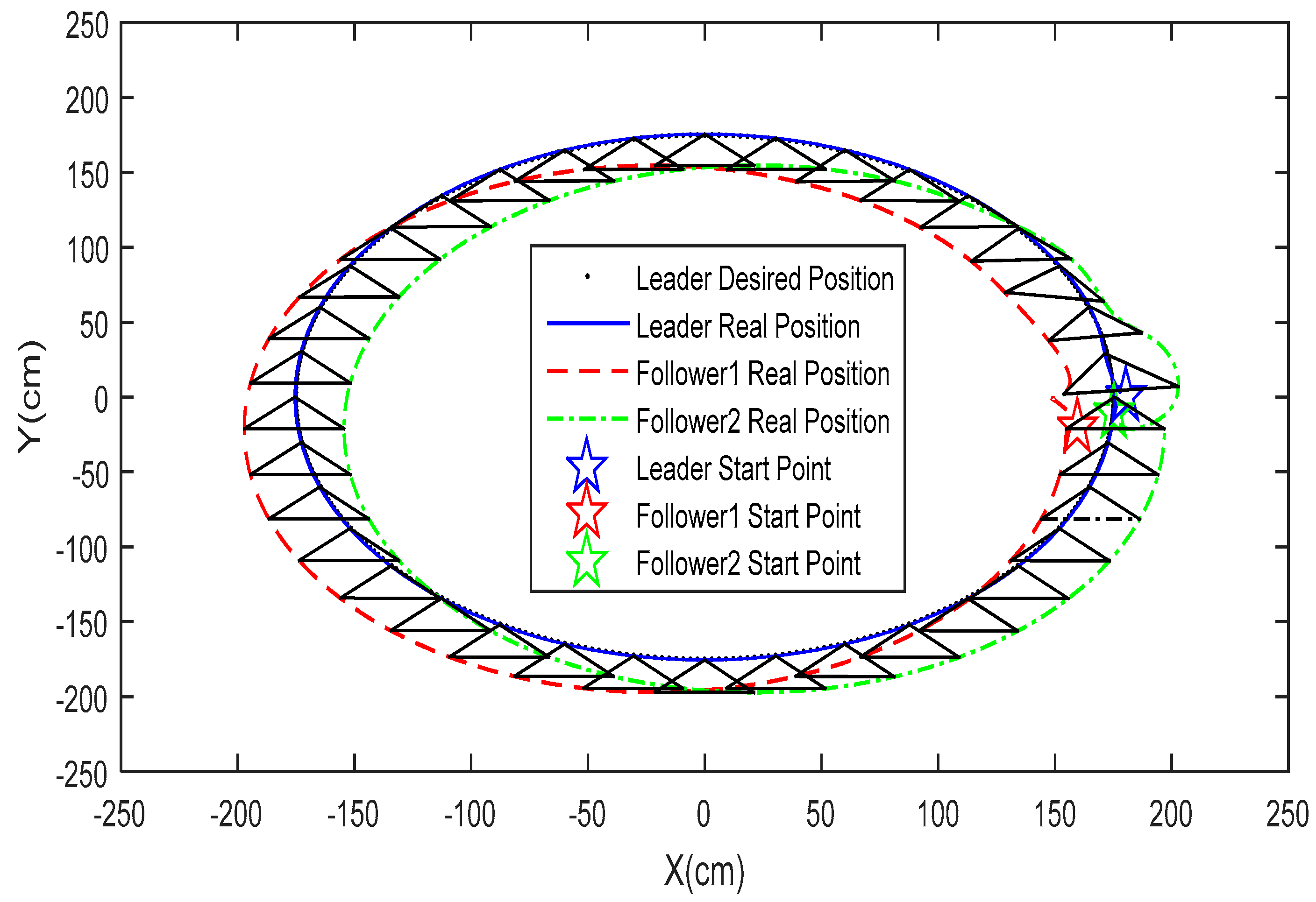
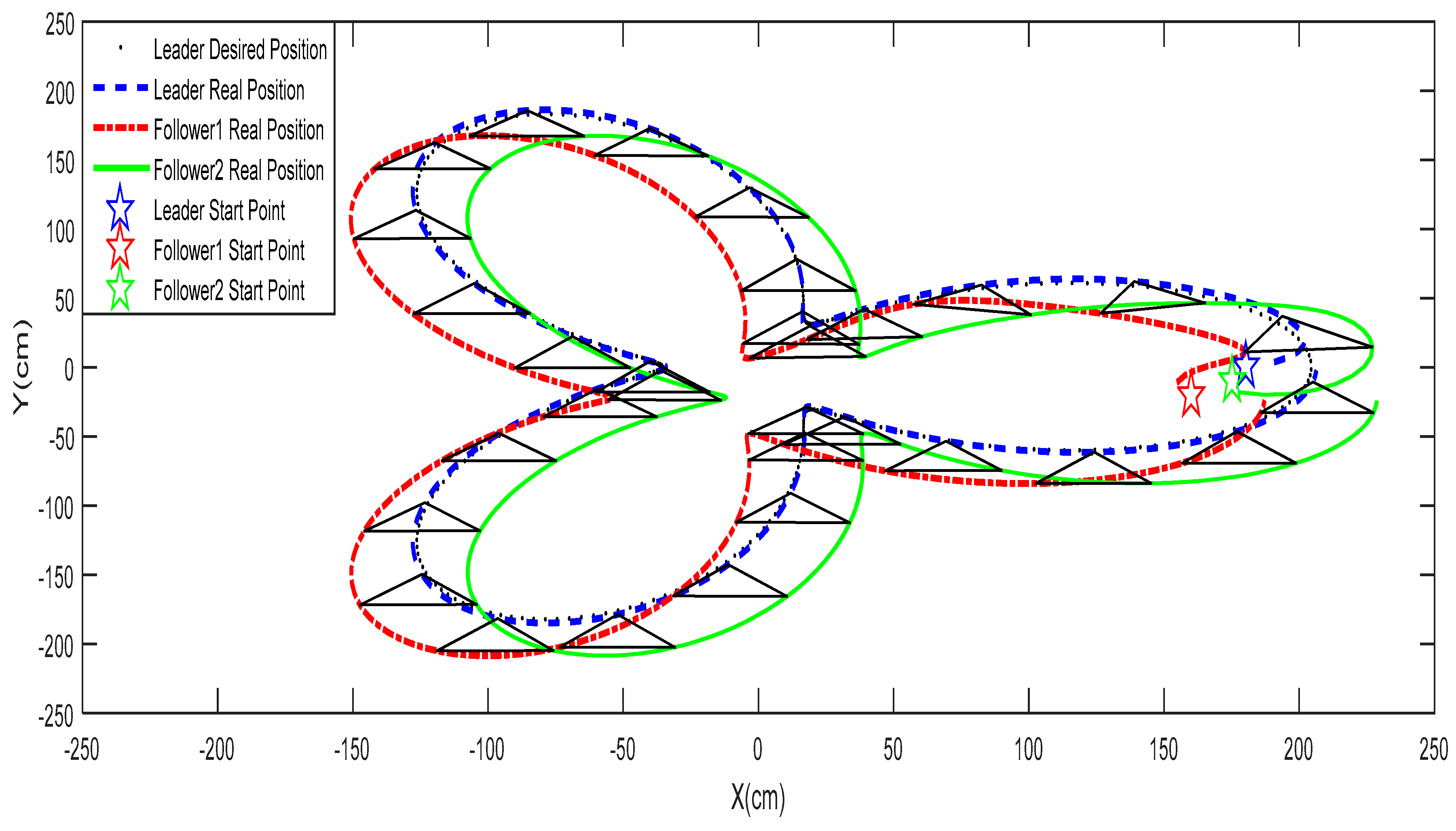
3.3. Leader-Follower Formation Control of Networked Mobile Robots

The leader-follower model is the main trend of networked mobile robotics, where a leader robot and several follower robots are included in a multi-robot system [32]. For networked mobile robots, formation control is an important topic that the leader robot tracks the desired trajectory while the follower robots maintain the formation shape. Figure 8 depicts a leader-follower networked mobile robotic system to achieve triangular formation control with three robots.
In this paper, all mobile robots are independently controlled by using Equation (17) to accomplish leader-follower formation control, and the control parameters are self-tuned via the GA-KF-RBFNN paradigm. Compared to traditional consensus multiple robot systems with directed graph topology, the proposed broadcast leader-follower networked mobile robot system circumvents the delay problem. The position and orientation of the robots are broadcasted via the network. To maintain the desired formation shape, the geometrical relationship of the leader robot and follower robots in Figure 7 is calculated. Since the data flow is broadcasted online to every robot, the communication delay issues that occur in the consensus multiple robot system are therefore avoided. The proposed GA-KF-RBFNN self-evolving formation control for networked mobile robots not only reduces the system noises, but also avoids the communication delay.

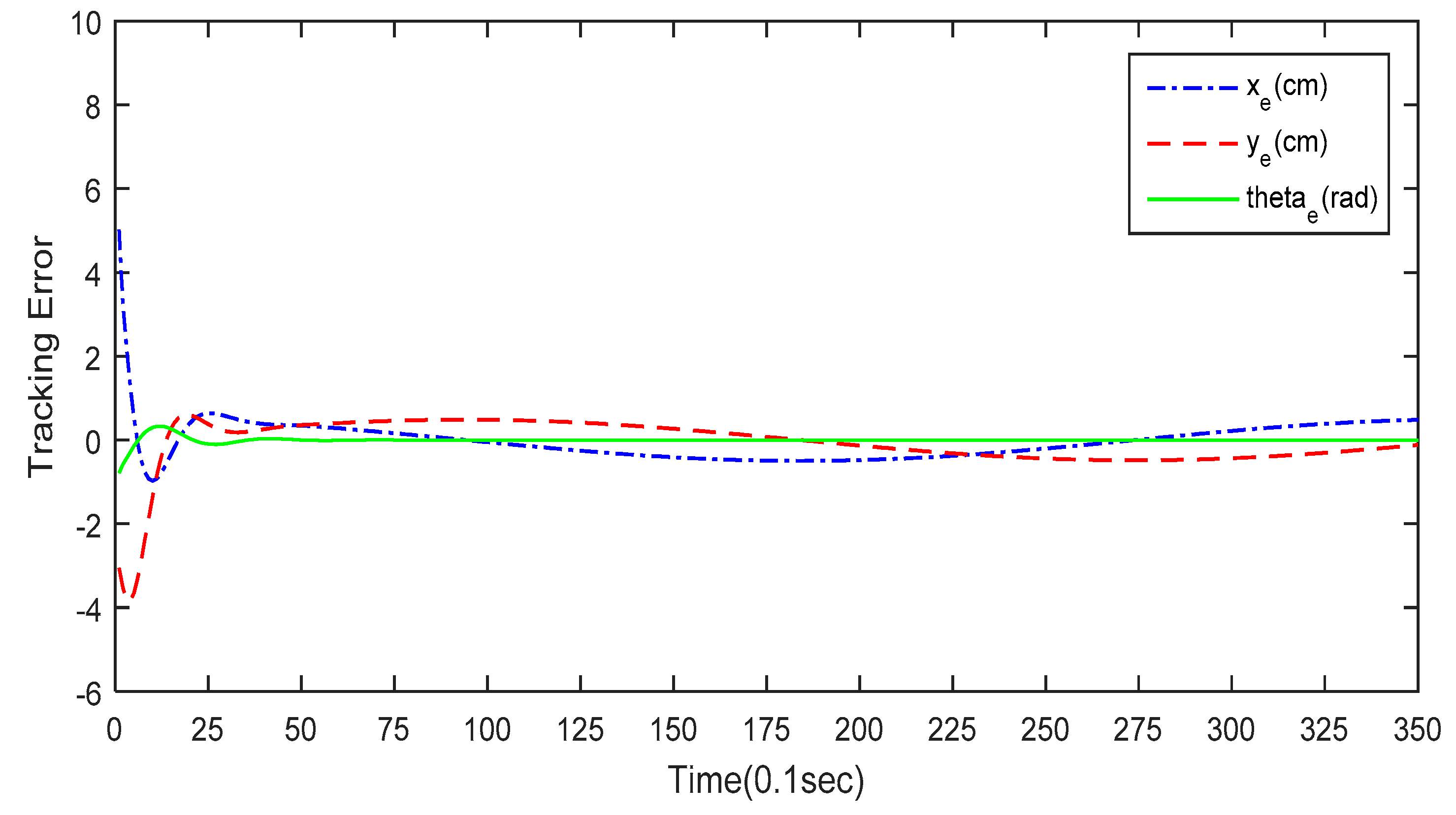
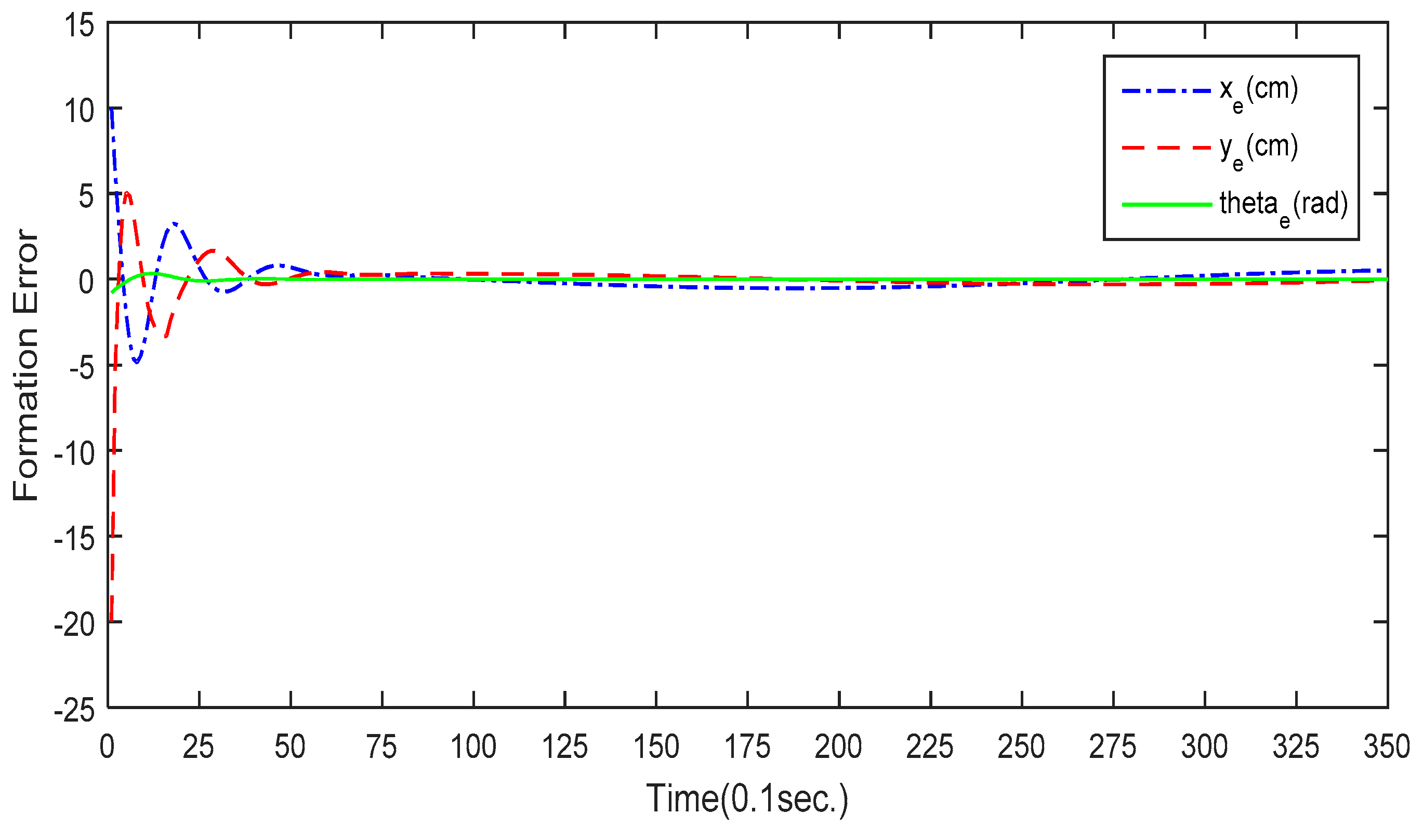
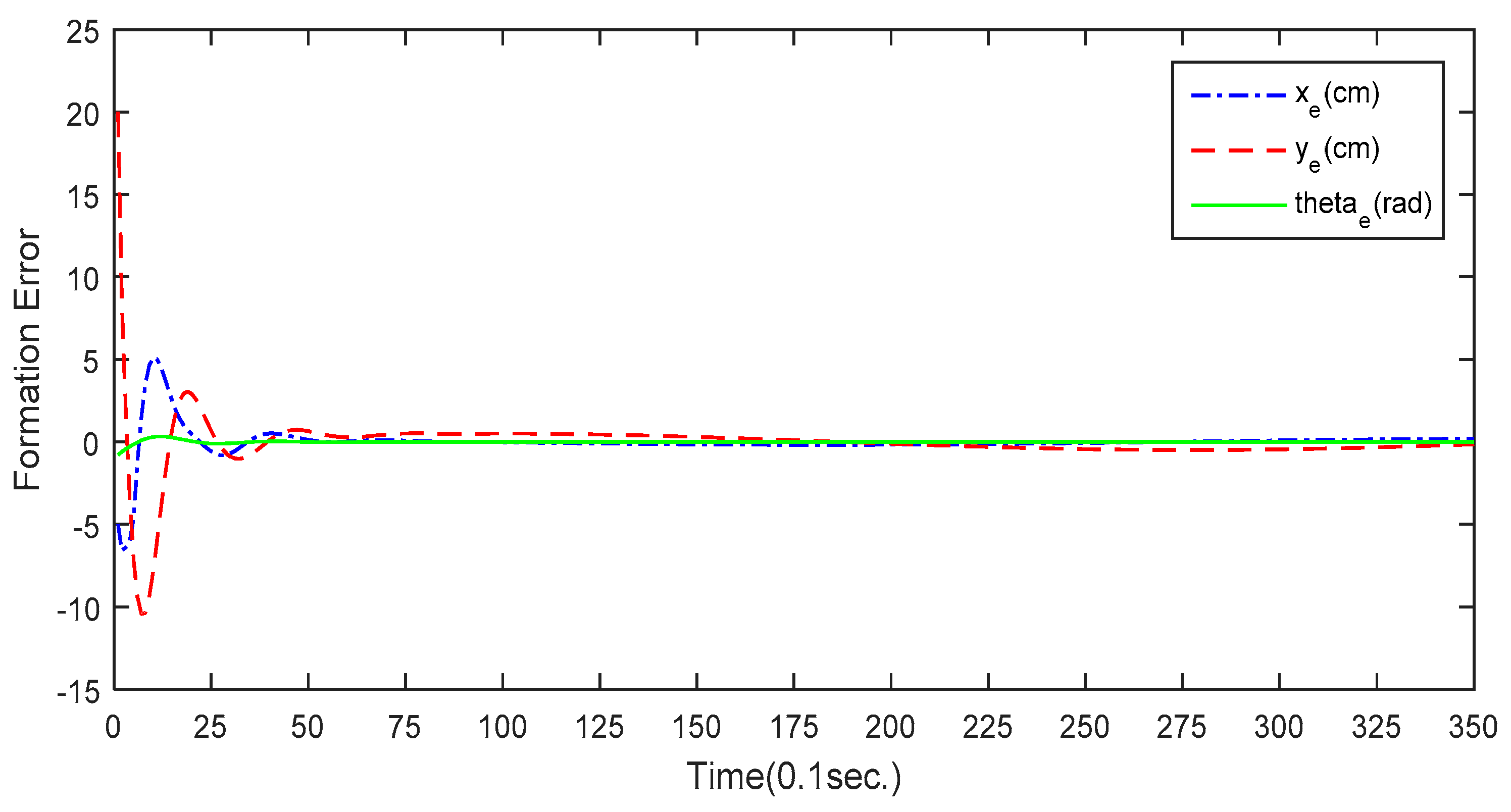
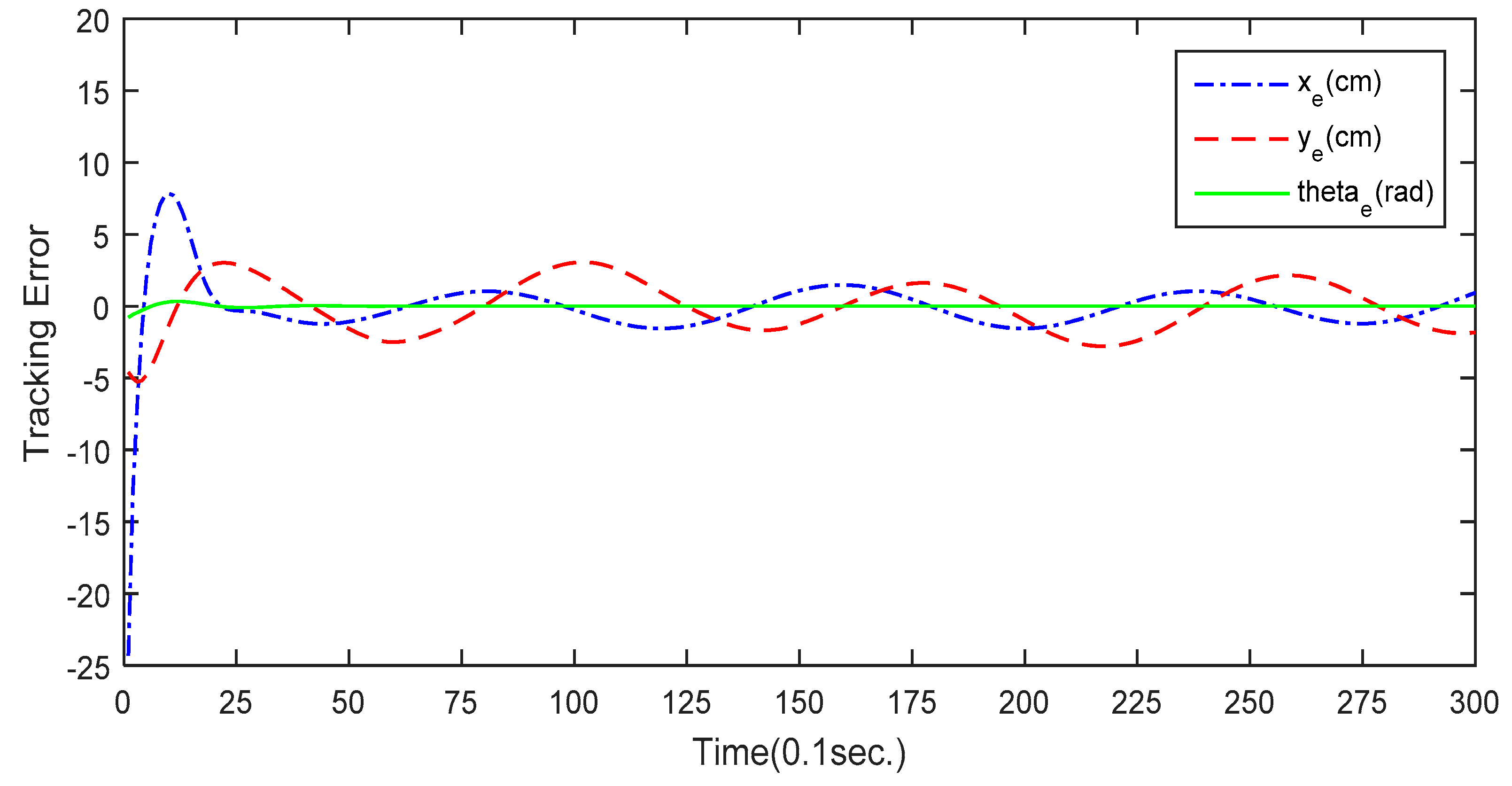
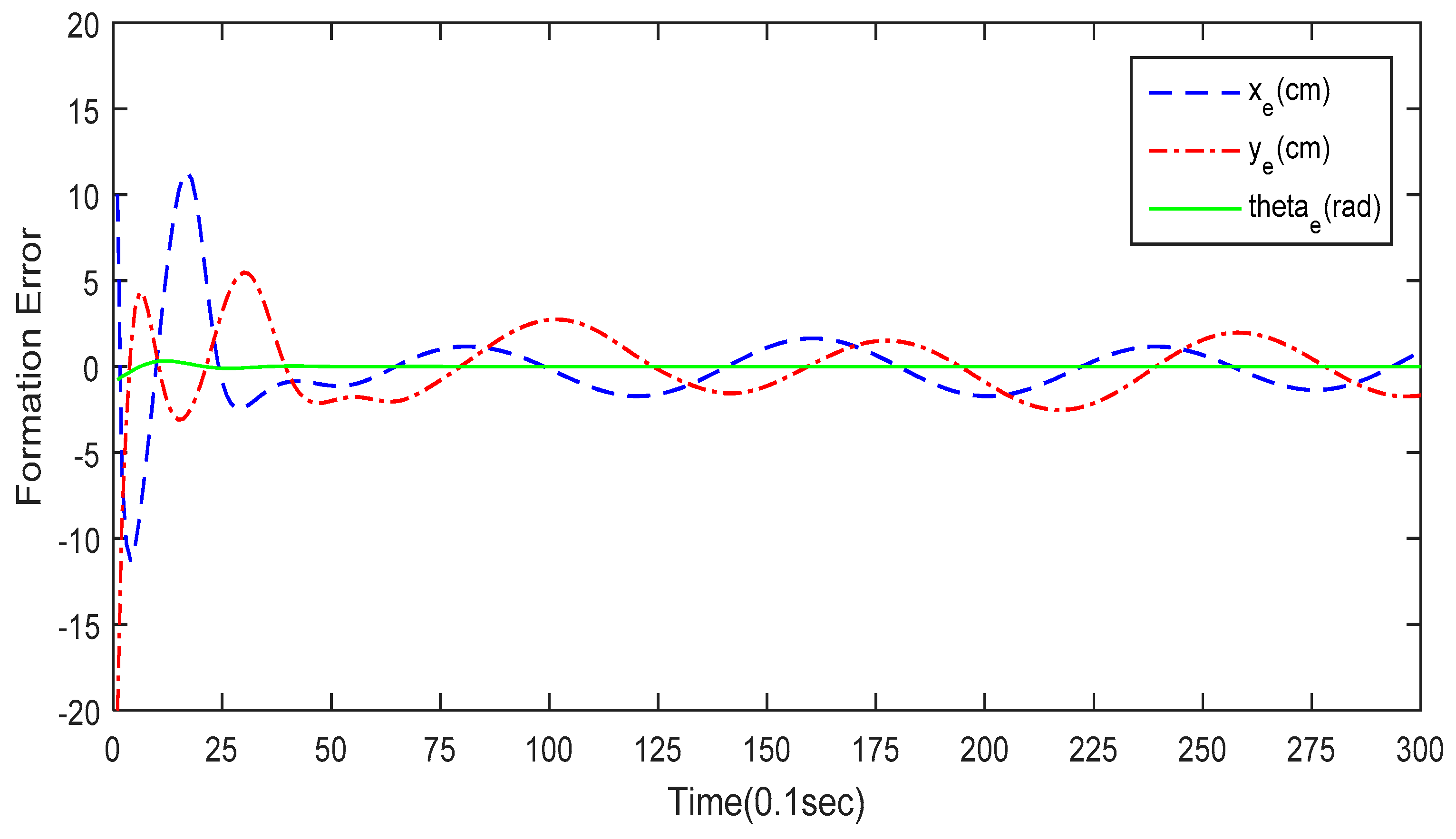
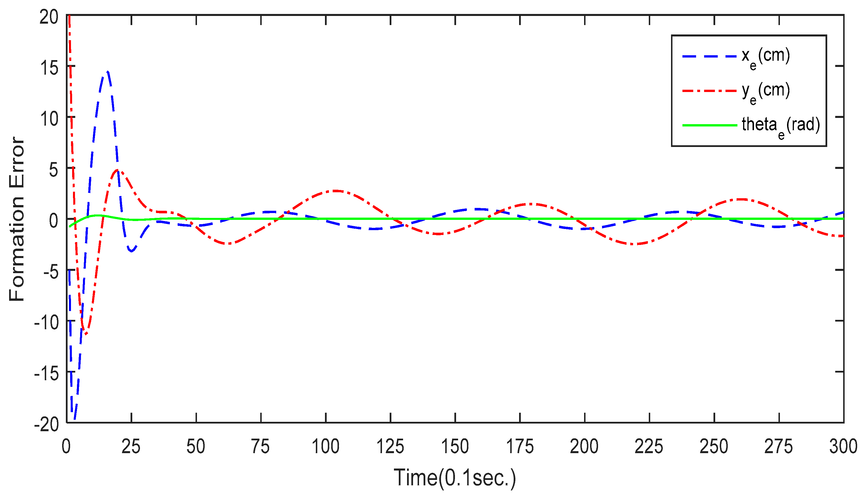
4. Simulations, Comparative Analysis, and Discussion

This section aims to conduct several simulations to examine the effectiveness of the proposed methods. The proposed networked mobile robot system consists of three four-wheeled Swedish omnidirectional mobile robots, including one leader and two follower mobile robots in a broadcast communication environment. The desired formation shape is triangular as shown in Figure 8. The system parameters in the proposed networked mobile robot system are L = 0.25 m and r = 5.08 cm.
The first simulation is conducted to demonstrate the performance of the circular formation control using the proposed GA-KF-RBFNN control approach. The number of iterations for the modified GA is 150, and the probabilities of crossover and mutation are determined by the Lévy flight. The circular trajectory for the leader robot is expressed as [ x r ( t ) y r ( t ) θ r ( t ) ] T = [ 1.75 cos ( ω i t )   m 1.75 sin ( ω i t )   m π / 4   rad ] T , ω i = 0.35   rad / sec . Figure 9 depicts the simulation result of the circular formation control. The three omnidirectional mobile robots are initially placed at different poses in the workspace. The desired trajectory for leader robot is a circular trajectory and the two follower robots aim to maintain a triangular formation. The tracking error of the leader mobile robot is presented in Figure 10. As shown in Figure 10, the leader mobile robot successfully tracks the desired circular trajectory in 4 s. Figure 11 depicts the formation error of follower robot #1 and Figure 12 depicts the formation error of follower robot #2. These simulation results demonstrate that the proposed GA-KF-RBFNN optimization is capable of accomplishing the self-learning formation control of networked mobile robotic systems.
The second simulation is provided to show the effectiveness of the proposed GA-KF-RBFNN formation control for daisy curve tracking. The desired trajectory of the leader robot is a special daisy curve with three petals, expressed by [ x r ( t ) y r ( t ) θ r ( t ) ] T = [ 1 2 + b ( a + r cos ( p ω i t ) ) cos ( ω i t )   m 1 2 + b ( a + r cos ( p ω i t ) ) sin ( ω i t )   m π / 4   rad ] T , b = 0.2 m, a = 0.6 m, r′ = 0.42 m, p = 3, and ω i = 0.35   rad / sec . To illustrate the noise reduction capability of the proposed GA-KF-RBFNN self-learning controller, a Gaussian noise is added into the process and measurement phases. Figure 13 presents the simulation result of daisy curve formation control using the proposed GA-KF-RBFNN and Figure 14 depicts the tracking error of the leader robot. Moreover, Figure 15 and Figure 16 present the formation error of follower robot #1 and follower robot #2, respectively, for daisy curve formation control. Both the tracking performance and formation behavior are guaranteed. These simulation results clearly indicate that the proposed metaheuristic GA-KF-RBFNN self-evolving control scheme with noise reduction achieves the formation control task for networked mobile robots. This approach outperforms the traditional consensus control methods where the uncertainty and self-adaptation are not considered.
In order to provide a comparative analysis to illustrate the merits of the proposed methods over other existing approaches, Table 1 lists the comparison of the proposed GA-KF-RBFNN formation control and traditional controllers. As shown in Table 1, the proposed biologically-inspired GA-KF-RBFNN learning and adaptation for self-evolving of networked mobile robots is superior to the traditional formation control methods. With the modified GA metaheuristics and Kalman filter, both the noise and delay problem are avoided. The proposed GA-KF-RBFNN formation control strategy is applicable to all kinds of mobile robots, including different-drive [36] and three-wheeled mobile robotic systems.

5. Conclusions

This paper has presented a biologically-inspired GA-KF-RBFNN learning and adaptation method for the self-evolving control of networked mobile robots. The Kalman filter algorithm is employed to develop a self-learning RBFNN by considering uncertainty and noises. Moreover, the structure of the proposed KF-RBFNN is optimally initialized by means of the modified GA in which a Lévy flight strategy is applied. With the derived kinematic model of a four-wheeled omnidirectional mobile robot and broadcast leader-follower model, the GA-KF-RBFNN is utilized to design a self-evolving motion control law for a networked mobile robotic system. This approach overcomes the problem of communication delay found in conventional consensus networked robotic systems. Simulation results illustrate the merits of the proposed intelligent networked mobile robot system which uses a GA-KF-RBFNN to achieve self-learning formation control and consider the uncertainty and noise.

Author Contributions

Conceptualization, methodology, analysis, writing—review and editing, S.S.-D.X. and H.-C.H.; Experiments, T.-C.C. and S.-K.L.

Funding

This research was funded by the Ministry of Science and Technology, Taiwan, under grant number MOST 107-2221-E-011-145, MOST 106-2221-E-197-002 and MOST 107-2221-E-197-028.

Conflicts of Interest

The authors declare no conflict of interest.

References

  1. Liu, Y.; Gao, J.; Shi, X.; Jiang, C. Decentralization of virtual linkage in formation control of multi-agents via consensus strategies. Appl. Sci. 2018, 8, 2020. [Google Scholar] [CrossRef]
  2. Keviczky, T.; Borrelli, F.; Fregene, K.; Godbole, D.; Balas, G. Decentralized receding horizon control and coordination of autonomous vehicle formations. IEEE Trans. Control Syst. Technol. 2008, 16, 19–33. [Google Scholar] [CrossRef]
  3. Qian, D.; Xi, Y. Leader-follower formation maneuvers for multi-robot systems via derivative and integral terminal sliding mode. Appl. Sci. 2018, 8, 1045. [Google Scholar] [CrossRef]
  4. Qu, Z.; Wang, J.; Hull, R.A.; Martin, J. Cooperative control design and stability analysis for multi-agent systems with communication delays. In Proceedings of the 2006 IEEE International Conference of Robotics and Automation, Orlando, FL, USA, 15–19 May 2006; pp. 970–975. [Google Scholar]
  5. Kantaros, Y.; Zavlanos, M.M. Global planning for multi-robot communication networks in complex environments. IEEE Trans. Robot. 2016, 32, 1045–1061. [Google Scholar] [CrossRef]
  6. Pan, L.; Lu, Q.; Yin, K.; Zhang, B. Signal source localization of multiple robots using an event-triggered communication scheme. Appl. Sci. 2018, 8, 977. [Google Scholar] [CrossRef]
  7. Ferrari-Trecate, G.; Galbusera, L.; Marciandi, M.P.E.; Scattolini, R. Model predictive control schemes for consensus in multi-agent systems with single and double integrator dynamics. IEEE Trans. Autom. Control 2009, 54, 2560–2572. [Google Scholar] [CrossRef]
  8. Dong, F.; Lei, X.; Chou, W. The adaptive radial basis function neural network for small rotary-wing unmanned aircraft. IEEE Trans. Ind. Electron. 2014, 61, 4808–4815. [Google Scholar]
  9. Yang, C.; Li, Z.; Cui, R.; Xu, B. Neural network-based motion control of an underactuated wheeled inverted pendulum model. IEEE Trans. Neural Netw. Learn. Syst. 2014, 25, 2004–2016. [Google Scholar] [CrossRef] [PubMed]
  10. Khosravi, H. A novel structure for radial basis function networks-WRBF. Neural Process. Lett. 2012, 35, 177–186. [Google Scholar] [CrossRef]
  11. Dash, C.S.K.; Dash, A.P.; Cho, S.B.; Wang, G.N. DE+RBFNs based classification: A special attention to removal of inconsistency and irrelevant features. Eng. Appl. Artif. Intell. 2013, 26, 2315–2326. [Google Scholar] [CrossRef]
  12. Chang, G.W.; Chen, C.I.; Teng, Y.F. Radial-basis-function-based neural network for harmonic detection. IEEE Trans. Ind. Electron. 2010, 57, 2171–2179. [Google Scholar] [CrossRef]
  13. Tong, C.C.; Ooi, E.T.; Liu, J.C. Design a RBF neural network auto-tuning controller for magnetic levitation system with Kalman filter. In Proceedings of the 2015 IEEE/SICE International Symposium on System Integration (SII), Nagoya, Japan, 11–13 December 2015; pp. 528–533. [Google Scholar]
  14. Hamid, K.R.; Talukder, A.; Islam, A.K. Implementation of fuzzy aided Kalman filter for tracking a moving object in two-dimensional space. Int. J. Fuzzy Log. Intell. Syst. 2018, 18, 85–96. [Google Scholar] [CrossRef]
  15. Ko, N.Y.; Jeong, S.; Bae, Y. Sine rotation vector method for attitude estimation of an underwater robot. Sensors 2013, 16, 1213. [Google Scholar] [CrossRef]
  16. Lu, X.; Wang, L.; Wang, H.; Wang, X. Kalman filtering for delayed singular systems with multiplicative noise. IEEE/CAA J. Autom. Sin. 2016, 3, 51–58. [Google Scholar]
  17. Wang, S.; Feng, J.; Tse, C. Analysis of the characteristic of the Kalman gain for 1-D chaotic maps in cubature Kalman filter. IEEE Signal Process. Lett. 2013, 20, 229–232. [Google Scholar] [CrossRef]
  18. Foley, C.; Quinn, A. Fully probabilistic design for knowledge transfer in a pair of Kalman filters. IEEE Signal Process. Lett. 2018, 25, 487–490. [Google Scholar] [CrossRef]
  19. Xie, S.; Xie, Y.; Huang, T.; Gui, W.; Yang, C. Generalized predictive control for industrial processes based on neuron adaptive splitting and merging RBF neural network. IEEE Trans. Ind. Electron. 2019, 66, 1192–1202. [Google Scholar] [CrossRef]
  20. Gutiérrez, P.A.; Hervas-Martinez, C.; Martínez-Estudillo, F.J. Logistic regression by means of evolutionary radial basis function neural networks. IEEE Trans. Neural Netw. 2011, 22, 246–263. [Google Scholar] [CrossRef] [PubMed]
  21. Huang, F.; Zhang, W.; Chen, Z.; Tang, J.; Song, W.; Zhu, S. RBFNN-based adaptive sliding mode control design for nonlinear bilateral teleoperation system under time-varying delays. IEEE Access 2019, 7, 11905–11912. [Google Scholar] [CrossRef]
  22. Zao, Y.; Zheng, Z. A robust adaptive RBFNN augmenting backstepping control approach for a model-scaled helicopter. IEEE Trans. Control Syst. Technol. 2015, 23, 2344–2352. [Google Scholar]
  23. Tian, J.; Li, M.; Chen, F.; Feng, N. Learning subspace-based RBFNN using coevolutionary algorithm for complex classification tasks. IEEE Trans. Neural Netw. Learn. Syst. 2016, 27, 47–61. [Google Scholar] [CrossRef] [PubMed]
  24. Chang, G.W.; Shih, M.F.; Chen, Y.Y.; Liang, Y.J. A hybrid wavelet transform and neural-network-based approach for modelling dynamic voltage-current characteristics of electric arc furnace. IEEE Trans. Power Deliv. 2014, 29, 815–824. [Google Scholar] [CrossRef]
  25. Zhao, Y.; Ye, H.; Kang, Z.S.; Shi, S.S.; Zhou, L. The recognition of train wheel tread damages based on PSO-RBFNN algorithm. In Proceedings of the 2012 8th International Conference on Natural Computation, Chongqing, China, 29–31 May 2012; pp. 1093–1095. [Google Scholar]
  26. Wei, Z.Q.; Hai, X.Z.; Jian, W. Prediction of electricity consumption based on genetic algorithm-RBF neural network. In Proceedings of the 2010 2nd International Conference on Advanced Computer Control, Shenyang, China, 27–29 March 2010; Volume 5, pp. 339–342. [Google Scholar]
  27. Wei, H.; Tang, X.S. A genetic-algorithm-based explicit description of object contour and its ability to facilitate recognition. IEEE Trans. Cybern. 2015, 45, 2558–2571. [Google Scholar] [CrossRef] [PubMed]
  28. Huang, H.C. FPGA-based hybrid GA-PSO algorithm and its application to global path planning for mobile robots. Przeglad Elektrotechniczny 2012, 7, 281–284. [Google Scholar]
  29. Ding, S.F.; Xu, L.; Su, C.Y.; Jin, F.X. An optimizing method of RBF neural network based on genetic algorithm. Neural Comput. Appl. 2012, 21, 333–336. [Google Scholar] [CrossRef]
  30. Chou, C.J.; Chen, L.F. Combining neural networks and genetic algorithms for optimising the parameter design of the inter-metal dielectric process. Int. J. Prod. Res. 2012, 50, 1905–1916. [Google Scholar] [CrossRef]
  31. Marshall, J.A.; Broucke, M.E.; Francis, B.A. Formations of vehicles in cyclic pursuit. IEEE Trans. Autom. Control 2004, 49, 1963–1974. [Google Scholar] [CrossRef]
  32. Oh, K.K.; Park, M.C.; Ahn, H.S. A survey of multi-agent formation control. Automatica 2015, 53, 424–440. [Google Scholar] [CrossRef]
  33. Alonso-Mora, J.; Baker, S.; Siegwart, R. Multi-robot navigation in formation via sequential convex programming. In Proceedings of the IEEE/RSJ International Conference on Intelligent Robots and Systems, Hamburg, Germany, 28 September–2 October 2015. [Google Scholar]
  34. Lee, H.C.; Roh, B.S.; Lee, B.H. Multi-hypothesis map merging with sinogram-based PSO for multi-robot systems. Electron. Lett. 2016, 52, 1213–1214. [Google Scholar] [CrossRef]
  35. Tsai, C.C.; Chen, Y.S.; Tai, F.C. Intelligent adaptive distributed consensus formation control for uncertain networked heterogeneous Swedish-wheeled omnidirectional multi-robots. In Proceedings of the Annual Conference of the Society of Instrument and Control Engineers of Japan (SICE), Tsukuba, Japan, 20–23 September 2016; pp. 154–159. [Google Scholar]
  36. Tiep, D.K.; Lee, K.; Im, D.Y.; Kwak, B.; Ryoo, Y.J. Design of fuzzy-PID controller for path tracking of mobile robot with differential drive. Int. J. Fuzzy Log. Intell. Syst. 2018, 18, 220–228. [Google Scholar] [CrossRef]
Figure 1. Structure of the classical Kalman filter.
Applsci 09 01034 g001
Figure 2. Structure of the classical RBFNN (Radial Basis Function Neural Network).
Applsci 09 01034 g002
Figure 3. Block diagram of the RBFNN control scheme.
Applsci 09 01034 g003
Figure 4. Block diagram of the KF-RBFNN control scheme.
Applsci 09 01034 g004
Figure 5. Flowchart of evolutionary GA.
Applsci 09 01034 g005
Figure 6. Geometry of the omnidirectional mobile robot with four Swedish wheels.
Applsci 09 01034 g006
Figure 7. Block diagram of the GA-KF-RBFNN redundant control scheme for mobile robot.
Applsci 09 01034 g007
Figure 8. Leader-follower formation control with three mobile robots.
Applsci 09 01034 g008
Figure 9. Simulation result of circular formation control.
Applsci 09 01034 g009
Figure 10. Tracking error of the leader mobile robot for circular formation control.
Applsci 09 01034 g010
Figure 11. Formation error of follower robot #1 for circular formation control.
Applsci 09 01034 g011
Figure 12. Formation error of follower mobile robot #2 for circular formation control.
Applsci 09 01034 g012
Figure 13. Simulation result for the daisy curve formation control.
Applsci 09 01034 g013
Figure 14. Tracking error of the leader mobile robot for daisy curve formation control.
Applsci 09 01034 g014
Figure 15. Formation error of follower robot #1 for daisy curve formation control.
Applsci 09 01034 g015
Figure 16. Formation error of follower robot #2 for daisy curve formation control.
Applsci 09 01034 g016
Table 1. A comparative analysis of the formation controllers for networked robots.
Evolutionary StrategyNoise ReductionDistributed FormationLeader-Follower ApproachConsensus Delayed FormationOmnidirectional Capability
[1,2]NoNoYesYesYesNo
[3,4,5,6]NoNoYesYesYesNo
[7,8,9]NoNoYesYesYesNo
[10,11,12,13]NoNoYesYesYesNo
[31,32,33,34]NoNoYesYesYesNo
This StudyYesYesYesYesNoYes

