Article

A Compressed Equivalent Source Method Based on Equivalent Redundant Dictionary for Sound Field Reconstruction

1
State Key Laboratory of Mechanical Transmission, Chongqing University, Chongqing 400044, China
2
College of Automotive Engineering, Chongqing University, Chongqing 400044, China
*
Author to whom correspondence should be addressed.
Appl. Sci. 2019, 9(4), 808; https://doi.org/10.3390/app9040808
Submission received: 23 January 2019 / Revised: 18 February 2019 / Accepted: 20 February 2019 / Published: 25 February 2019
(This article belongs to the Section Acoustics and Vibrations)

Abstract

:

Featured Application

Authors are encouraged to provide a concise description of the specific application or a potential application of the work. This section is not mandatory.

Abstract

The equivalent source method (ESM) based on compressive sensing (CS) requires that the source has a sparse or approximately sparse representation in a suitable basis or dictionary. However, in practical applications, it is not easy to find the appropriate basis or dictionary due to the indeterminate characteristics of the source. To solve this problem, an equivalent redundant dictionary is constructed, which contains two core parts: one is the equivalent dictionary used in the CS-based ESMs under the sparse assumption, and the other one is the orthogonal basis obtained by the singular value decomposition (SVD). On this foundation, a method named compressed ESM based on the equivalent redundant dictionary (ERDCESM) is proposed to enhance the performances of source field reconstruction for different types of sources. Moreover, inspired by the idea of functional beamforming (FB), ERDCESM with order v (ERDCESM- v ) can possess a high dynamic range when detecting the source location. The numerical simulations are carried out at different frequencies to evaluate the performance of the proposed method, and the results suggest that the proposed method performs well both for sparse and even spatially extended sources. The validity and practicality of the proposed method are also verified by the experimental results.

Graphical Abstract

1. Introduction

The equivalent source method (ESM) based on Nearfield acoustic holography (NAH) is a powerful tool for identifying sound sources and visualizing sound fields [1,2,3]. The method is based on the fundamental idea that the actual sound field can be approximated as the superposition of waves radiated by a series of discrete simple sources. In the ESM, an equation relating the measured pressures to the equivalent sources is established, and the source strengths vector can be determined by matching the boundary conditions on the source or on the hologram plane. Recently, the ESM is appealing in the field of NAH for its simplicity, computational efficiency, and the adaptability to arbitrarily shaped sources [4,5,6].
The ESM, as well as other holography methods [7,8,9,10], generally leads to underdetermined problems, since the number of microphones is limited in most acoustic studies. The classical way of solving the problem is in a least-squares (LS) sense, by means of Tikhonov regularized Moore–Penrose pseudoinverse with regularization parameter λ . A combined criterion for selecting the parameter λ is described by Leclere in Ref. [11]. However, the above conventional ESM with Tikhonov regularization (TRESM) only gives the minimum-norm solution, which tends to unduly spread errors in the solution space.
In recent years, some compressive sensing (CS) methods have been widely used in the field of signal/image processing [12,13,14]. CS is an effective signal acquisition and processing technique based on the idea that data often have a sparse representation in a suitable basis or dictionary, i.e., they can be described only with few non-zero coefficients [15]. In source identification, Chardon et al. [16] first introduced the concept of CS to NAH and constructed a sparsity framework for NAH. After that, Fernandez-Grande et al. applied the CS theory to a wave expansion method based on measurements with a spherical microphone array [17]. E. Fernandez-Grande has presented a detailed study of the compressive ESM (CESM) [18]. When the source is distributed sparsely, the CS theory can be directly applied to NAH to reduce the number of measurement points or to extend the frequency range, which has been intensively studied in many literatures [19,20,21]. When the source is not distributed sparsely (e.g., the spatially extended source), it is necessary to construct an appropriate basis or dictionary to sparsely decompose the sound field so that the sparsity condition required by the CS theory can be fulfilled. In this case, two typical methods, named the total generalized variation regularization (TGV) [22] and the compressed modal equivalent point source method (CMESM) [23], are introduced. However, in most of the practical applications, the characteristics of the source are not clear. Therefore, it is difficult to choose a suitable basis or dictionary for the sparse representation of source distribution.
In this paper, a compressed ESM based on an equivalent redundant dictionary (ERDCESM) is proposed, which is applicable both for sparse and even spatially extended sources. The method aims at enhancing the performance of source field reconstruction for different types of sources. In this method, the constructed equivalent redundant dictionary contains two core modules: one is a series of orthogonal basis of sound field obtained by employing the singular value decomposition (SVD), and the other one is the equivalent dictionary used in the CS-based ESMs under the sparse assumption. Compared with CMESM and CESM, ERDCESM is more flexible for different types of sources. Moreover, combining the advantages of functional beamforming (FB) [24,25], ERDCESM with order v (ERDCESM- v ) is applied to make further improvement of the dynamic range when detecting the source location.
The remainder of this paper is organized as follows. In Section 2, the basic theory of ESM-based NAH is provided first, and then a theoretical derivation of the proposed method is described. In Section 3, numerical simulations including single-source and plate-source are implemented to evaluate the performance of the proposed method. Section 4 verifies the practicability of the proposed method by identifying the given sound sources. Finally, several conclusions are presented in Section 5.

2. Theory Background and Methodology

The method proposed in this paper is based on the ESM and CS theory. Firstly, rooted on the principle of ESM, the sound field model can be established. And then, two parts called an equivalent dictionary under the sparse assumption and a series of orthogonal basis obtained by SVD are combined to form an equivalent redundant dictionary. On this foundation, ERDCESM is presented under the CS framework. Moreover, to further improve the dynamic range of sound source identification and location, a reformative method which takes advantage of FB is developed.

2.1. Description of the Equivalent Source Method

The principle of ESM is that the sound field radiated by an arbitrarily shaped source can be substituted by a number of equivalent sources on a fictitious plane. This method is not involved in the Fourier transform in the wave number domain, hence it can avoid “windowing effects” and “wraparound errors” fundamentally. The diagrammatic sketch of ESM is shown as Figure 1.
It is assumed that there are N virtual equivalent sources on equivalent source plane and M microphones on the measurement plane. The sound pressure at the   m -th measurement point can be expressed as Equation (1):
p ( m ) = n = 1 N g ( r m | r n ) q n
where g ( r m | r n ) is the monopole pressure–pressure transfer function linking the n -th equivalent source to the m -th microphone, and it can be expressed as in Equation (2) [26]:
g ( r m | r n ) = e x p ( j k || r m n || ) 4 π || r m n ||
where k   is the acoustic wavenumber (in rad/m), and   || r m n || is the distance between the considered source–microphone couple. Then, the relationship between measured sound pressure and equivalent source strengths can be described in matrix vector notation as Equation (3):
p = A q
where A = j ρ ω g ( r m | r n ) is the transfer matrix relating the measured pressures to the equivalent sources, ω is the angular frequency (in rad/s ), and ρ is the density of the fluid (in kg/m3). p (size M × 1 ) is the column vector that contains the pressures at the   M measurement points, and q (size N × 1 ) is the column vector that contains the source strengths.
The source strength vector q is typically obtained in a least-squares sense by minimizing the cost function, as seen in Equation (4) [11]:
Γ λ ( q ) = | | p A q | | 2 2 + λ | | q | | 2 2
where || · || 2 denotes l 2   norm. λ is the regularization parameter. Once the source strengths q   are obtained, the sound pressure on any reconstruction plane can be calculated as Equation (5):
P R = G q
where G is the transfer matrix relating the reconstruction points to the equivalent sources.

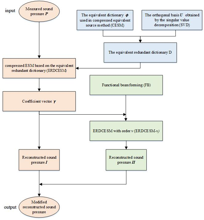
2.2. Compressed ESM Based on the Equivalent Redundant Dictionary

2.2.1. The Equivalent Dictionary Under the Sparse Assumption

When the actual sound sources are distributed sparsely, the source strengths q often have a sparse representation in some basis. In this condition, the equivalent source strengths can be expressed in the following form, as seen in Equation (6) [21]:
q = I α
where I is the identity matrix, which can be regarded as the sparse basis of equivalent source strengths.   α is the coefficient vector of the basis.
Then, the l 2   norm in the penalty term of Equation (4) can be replaced by a l 1   norm, i.e., see Equation (7):
argmin α p A I α 2 2 + λ α 1  
Once the coefficient α is solved , the sound pressure on the reconstruction plane can be obtained by the following formula of Equation (8):
P R = G q = G I α = ϕ α
where ϕ = G I denotes an equivalent dictionary.

2.2.2. Construction of the Equivalent Redundant Dictionary

When the actual sound sources are not sparse, it is necessary to construct an appropriate basis to sparsely decompose the sound field. In this paper, the SVD method is applied to determine this basis.
By applying the SVD to the transfer matrix G , Equation (5) can be rewritten as Equation (9) [27,28]:
P R = G q = U S V H q = i = 1 N u i λ i v i H v i q = i = 1 N u i α i = U β
where U and V are unitary matrices, and   u i and v i represent column vectors of   U and V , respectively. H denotes the conjugate transpose, S is a real diagonal matrix, and λ i denotes singular values.   β is the coefficient vector of the basis.
In Equation (9), U is an orthogonal matrix of singular vectors and contains a set of basis vectors of N-dimensional space, which has been well-studied in literature [11,27]. Similar to the method presented by Bi et al. [23], the basis can also be regarded as acoustic modes [29]. Since the modes are spatially continuous, U is especially suitable for the spatially extended sound source. The acoustic signal can be reconstructed well only by a few column vectors of U , which correspond to the large singular value. This enables the sparsity of the solution to be enhanced when the SVD is utilized, and therefore the ESM in the CS framework can be solved.
However, in most practical applications, the characteristics of the source are not clear [30,31]. It is difficult to choose a suitable basis or dictionary for the sparse representation of source distribution. To solve this problem, a new equivalent redundant dictionary, D = [ ϕ , U ] , is constructed by combining Equations (8) and (9). Therefore, the sound pressure on the reconstruction plane can be expressed as Equation (10):
P R = D Υ
In this equivalent redundant dictionary D , ϕ is the equivalent dictionary used in CESM, which is especially suitable for the sources distributed spatially sparse.   U can be viewed as “acoustic mode”, which is applicable for the spatially extended source. Therefore, by taking advantage of ϕ and U comprehensively, D is expected to be appropriate whether the sources are spatially sparse or spatially extended.
According to Equations (3) and (5), the pressure p can be reformulated as Equation (11):
p = A q = A ( G ) + P R
and substituting Equation (10) to Equation (11) yields Equation (12):
p = A ( G ) + P R = A ( G ) + D Υ = D e Υ
where D e = A ( G ) + D , and the superscript ”+” denotes the Moore–Penrose inverse.
Using the l 1   norm regularization, Equation (12) can be solved by minimizing the cost function as Equation (13):
Γ λ ( Υ ) = || p D e Υ || 2 2 + λ || Υ || 1  
Equation (13) is equivalent to the l 1   norm minimization problem, see Equation (14):
argmin Υ || Υ || 1     s u b j e c t   t o   || p D e Υ || 2 ε
where ε represents the tolerance.
According to Hald [20], the constraints in Equation (14) can be adjusted, and the problem is described by Equation (15):
argmin Υ || Υ || 1   s u b j e c t   t o   || ( D e ) H ( p D e Υ ) || 2 δ
where δ = σ || ( D e ) H p || 2 , and σ is a small number.
Equation (15) is the basis formulation of ERDCESM, which can be solved by CVX toolbox [32]. Once the coefficient Υ is obtained, the pressure can be reconstructed via Equation (10). Since the dictionary D in ERDCESM is a combination of ϕ   (it is suitable for the spatially sparse source) and U (it is suitable for the spatially extended source), the ERDCESM works well for different types of sources.

2.3. A Reformative Method Combining with Functional Beamforming

To further improve the dynamic range of sound source identification and location, the solution of Equation (10) can be reformulated by referring to functional beamforming (FB).
Firstly, the cross spectral matrix (CSM) of Υ is calculated with Equation (16) [24]:
C = Υ Υ H
Since C is nonnegative Hermitian matrix, the spectral decomposition of C can be written as Equation (17):
C = V d i a g ( γ 1 , , γ N ) V H
where V is the unitary matrix whose columns represent the eigenvectors of C .   γ 1 , , γ N are the eigenvalues.
The exponential matrix function of C is defined by Equation (18) [24]:
C 1 ν = V d i a g ( γ 1 1 ν , , γ N 1 ν ) V H
where v is a positive integer, which represents the order.
Based on FB [24,25], the sound pressure at the   i -th point on the reconstruction plane can be expressed as Equation (19):
Z i = ( D e i C 1 ν ( D e i ) H ) ν
where D e i represent column vectors of   D e .
It has to be mentioned that the output peaks values of Equation (19) may be smaller than the actual source amplitude. Therefore, to guarantee the true estimation of maximum pressure amplitude, it is suggested that the sound pressure on the reconstruction plane should be modified through combining Equations (10) and (19). Finally, the final result of ERDCESM- v is as the following Equation (20):
P o u t = { P R v = 0 Z i max ( | P R | ) max ( | Z i | ) v = 1 , 2 , 3 ,
To almost completely reconstruct the sound field, ERDCESM with order v = 0 is suitable. However, if there is a demand for identifying source location with high accuracy and wide dynamic range, ERDCESM with order v = 1 , 2 , 3 , . is recommended. So the application of ERDCESM- v is very flexible and also provides high-precision source localization.

3. Simulated Measurements

To compare the reconstruction performances of the four methods (TRESM, CESM, CMESM, and ERDCESM) for different types of sources, simulated measurements were carried out. For CESM, CMESM, and ERDCESM, the CVX toolbox was used for the l 1   norm optimization. For TRESM, the optimal regularization parameter was determined via the L-curve method [11]. In the measurements, a single source was selected to simulate the sparse source, and a simple supported plate was used as a type of spatially extended source. Simulations of ERDCESM- v were also implemented to verify the superiority of combining with FB.

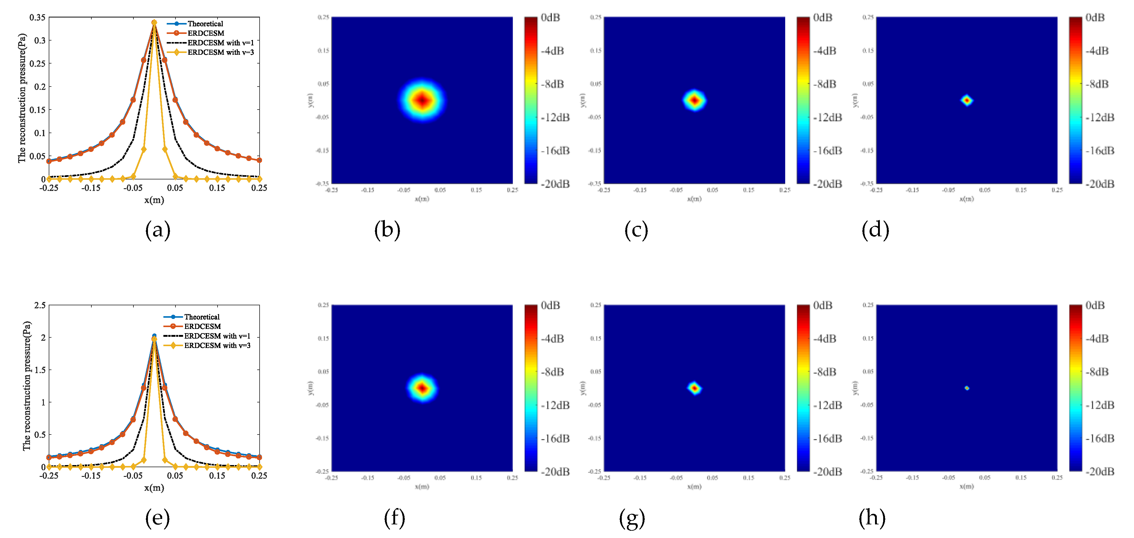
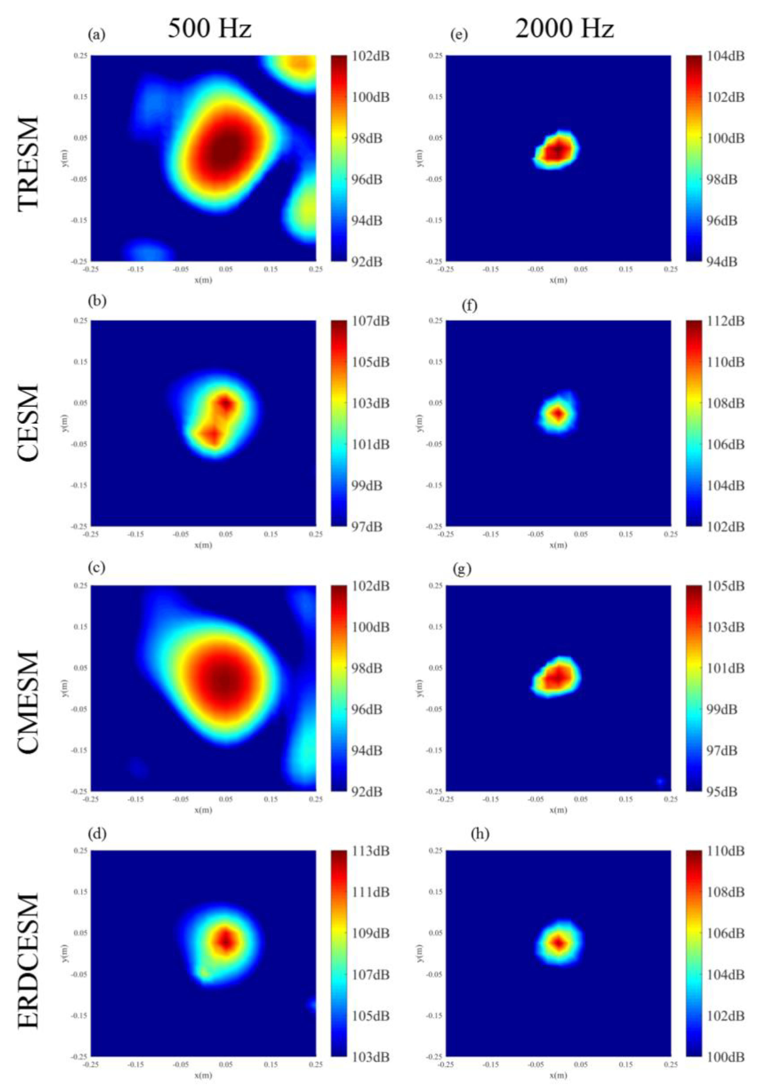
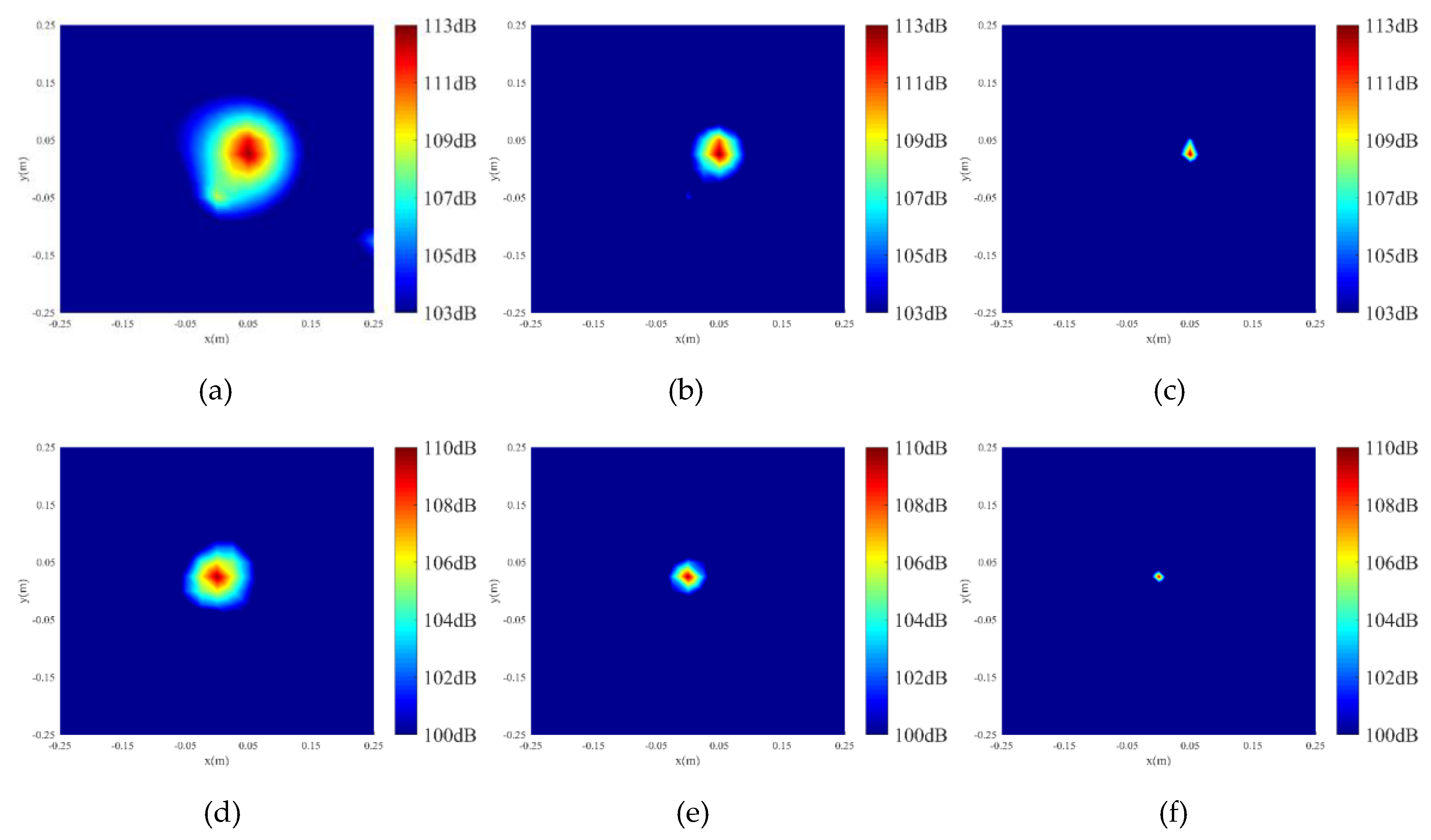
3.1. Single Sound Source

The aim of this simulation was to compare the reconstruction performances of the four methods for a single sound source. The source was placed at (0, 0, 0) m. The distance between the measurement plane and the origin of coordinates was 0.1 m, while the distance between the reconstruction plane and the origin of coordinates was 0.02 m. The equivalent source plane was located at 0.001 m from the real sources. Random noise with a signal-to-noise ratio (SNR) of 20 dB was added to the pressures to simulate the actual measurement. The reconstruction plane and equivalent source plane were meshed by 21 × 21   grids with a uniform interspacing of 0.025 m. There were 64 measurement points which were randomly selected from 441 points located on 21 × 21   grids (with 0.025 m intervals) to simulate a random array, as shown in Figure 2.
To quantitatively evaluate the performance of ERDCESM, the reconstruction error was defined as Equation (21):
L e r r o r = P r P t 2 P t 2 × 100 %  
where P t and P r are the theoretical and reconstructed pressure, respectively.
According to Equation (21), the reconstruction error for a single source in a frequency range from 50 Hz to 3000 Hz is shown in Figure 3. The results at each frequency were obtained 10 times to produce an average reconstruction error. It was observed that the reconstruction accuracy of ERDCESM and CESM were much higher than TRESM and CMESM. The results of CMESM were not satisfactory because, for the source that distributed sparsely in the space domain, its spatial acoustic modes were spatially continuous rather than sparse. In this condition, it was not appropriate to use the l 1   norm as a constraint term. The unsatisfactory reconstruction effect of TRESM was mainly due to insufficient measurement points. When the frequency range was higher than 500 Hz, the accuracy of ERDCESM was almost as good as that of CESM. Viewed as a whole, ERDCESM obtained a satisfactory reconstruction effect in a relatively wide frequency range.
Figure 4 illustrates the theoretical sound source map on the reconstruction plane and the corresponding maps calculated by TRESM, CESM, CMESM, and ERDCESM. For the source at 500 Hz, it is easy to see that ERDCESM and CESM have good consistency with the theoretical source map. The reconstructed source maps based on TRESM and CMESM present a hot-spot at the given position, which is much larger than that on the corresponding maps using other two methods. When the source was set at 2000 Hz, a similar conclusion could be derived that CESM and ERDCESM produced a better resolution than TRESM and CMESM.
To better and vividly illustrate the performance of ERDCESM- ν , Figure 5 shows the pressure distribution on the reconstruction plane at 500 and 2000 Hz. As can be seen from Figure 5a,e, with the order ν increasing, the identified peak sound pressure almost kept constant and approximated the theoretical value. For the source at 500 Hz, it was observed that although ERDCESM with order ν = 1 (Figure 5c) and ν = 3 (Figure 5d) could not fully reconstruct the sound pressure distribution, they could provide a more accurate source position than that of ERDCESM with ν = 0 (Figure 5b). When the source was at 2000 Hz, a similar conclusion was derived.

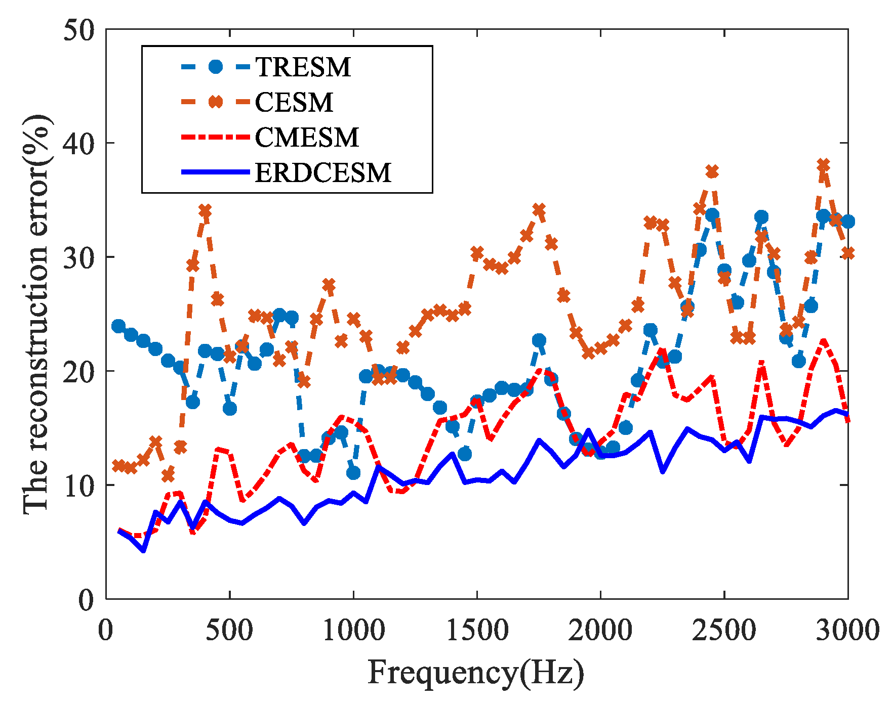
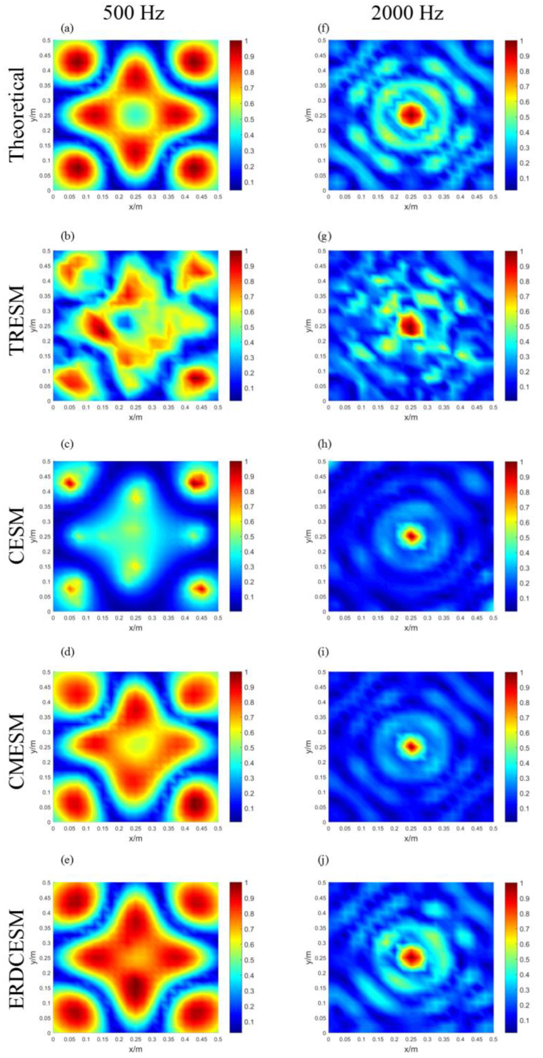
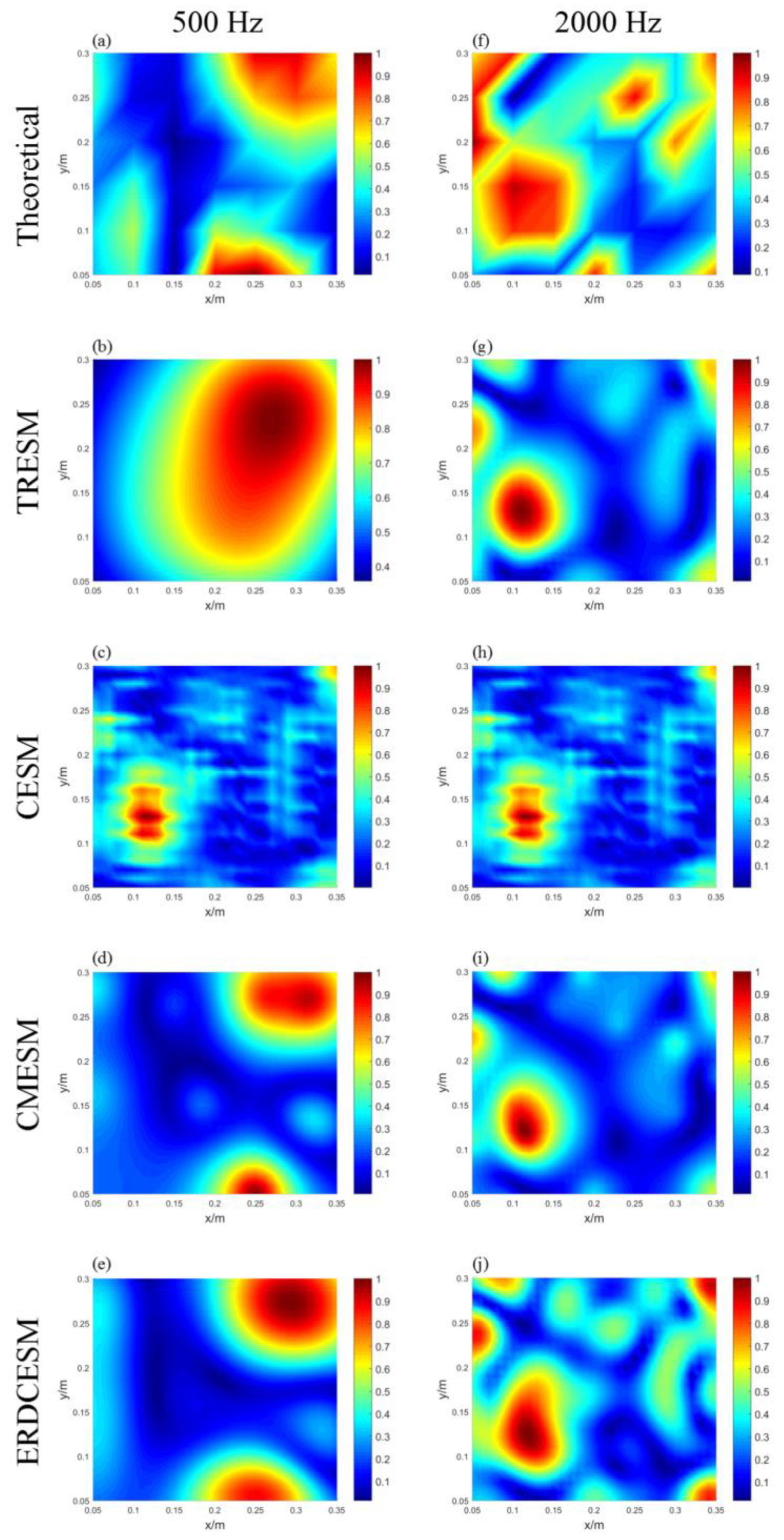
3.2. Simply supported plate

In this simulation, a 50 cm × 50 cm × 3 mm finite simply supported steel plate was used to test the performance of the proposed method. The plate was excited by point force of 1 N at the center. The radiated sound field was calculated by using the Rayleigh’s first integral. The measurement plane and reconstruction plane were meshed by 21 × 21   grids with a uniform interspacing of 0.025 m. The two planes were located 5 cm (measurement plane) and 2 cm (reconstruction plane) above the plate. There were 64 measurement points which were randomly selected from 441 points located on 21 × 21   grids (with a 0.025 m interval) to simulate a random array, as shown in Figure 2. The equivalent sources were distributed on a plane 0.001 m from the plate, with a grid of 21 × 21 and a uniform interspacing of 0.025 m. Random noise with an SNR of 20 dB was added to the pressures to simulate the actual measurement.
Figure 6 shows the reconstruction errors of the four methods over the frequency range of 50–3000 Hz. In a relatively wide frequency range, ERDCESM provided a better accuracy than the other three methods. The CESM performed well only at low frequencies (e.g., at 100 Hz, 200 Hz), and the error gradually became unacceptable with the increased frequency. The main reason resulting in this phenomenon was that the sparse basis of CESM disagreed with the spatially extended sound source, and the equivalent point source strengths could not be well-compressed. The difference between ERDCESM and CMESM was that ERDCESM possessed a complex-valued dictionary which contains more phase information, and consequently yielded better reconstruction effects for the same number of measurement points.
Sound source maps of simply supported plate at 500 Hz and 2000 Hz are presented in Figure 7. It can be seen that the reconstruction accuracy obtained by ERDCESM and CMESM match the theoretical one better than those obtained by TRESM and CESM. CESM provided less accurate reconstruction at these two frequencies. This was because the radiated sound field of simply supported plate was complex which lead to a worse spatial sparsity, and the sparse basis of CESM was not suitable. Therefore, to accurately reconstruct the sound field, the number of measurement points required by CESM was more than required by CMESM and ERDCESM. Moreover, in terms of sources distribution, ERDCESM had a more accurate reconstruction, compared with CMESM.
Using ERDCESM- ν , the comparison of sound pressure distributions with different orders at 500 Hz is shown in Figure 8. It can be seen that when ν = 1 , the identified sound pressure distribution was similar to that of the theoretical one (see the Figure 8b and Figure 7a). With the order ν increasing, the coverage of the identified acoustic center was narrowed gradually. Therefore, the maximum area of sound pressure distribution was located by increasing order ν , which provided direction for the optimization and improvement of structural panels. However, it was worth noting that some important sound pressure information could be lost (e.g., Figure 8d,   ν = 5) if the order ν was too large. Consequently, a smaller order ν was recommended for the sound source identification of structural panels.

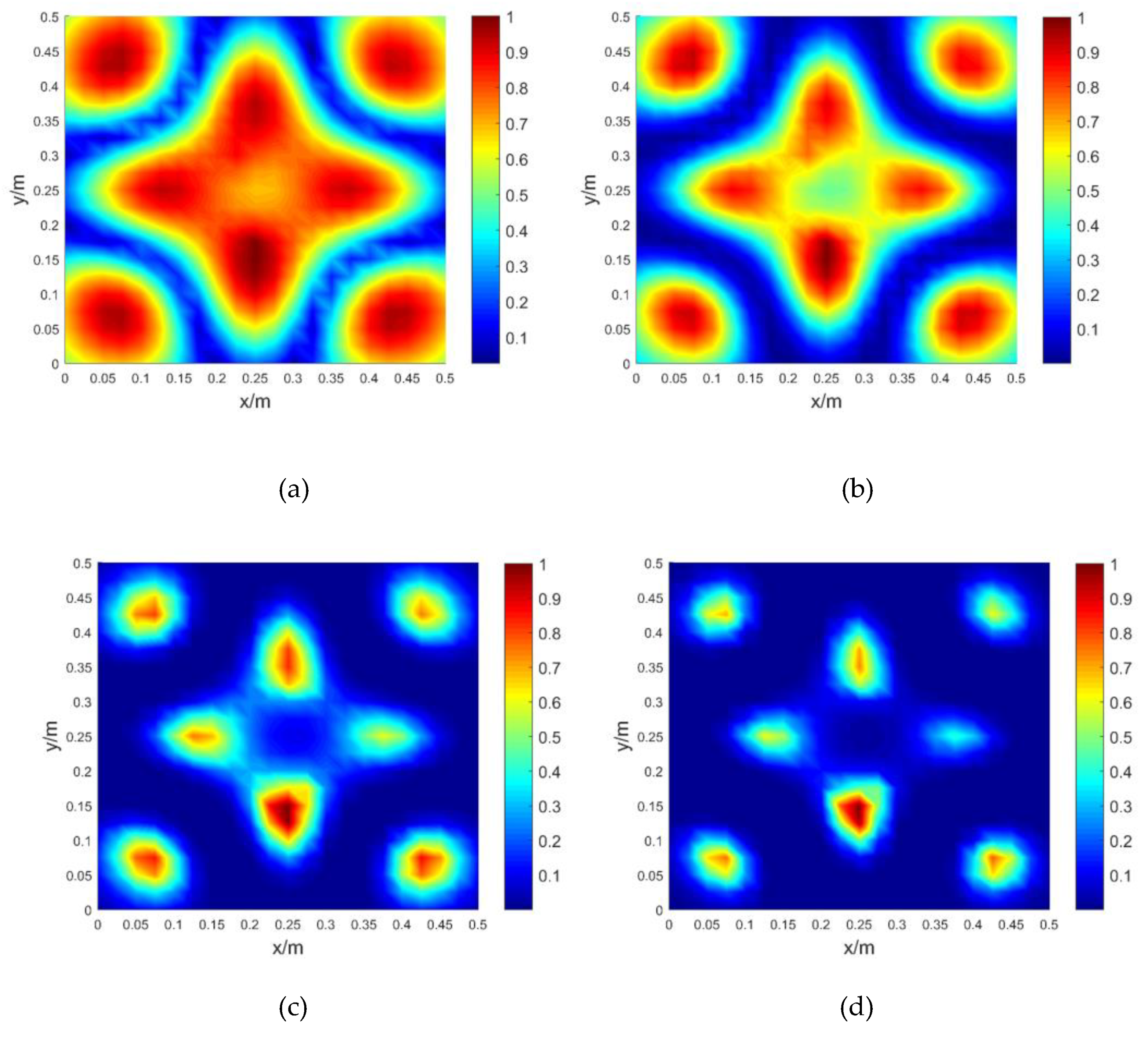
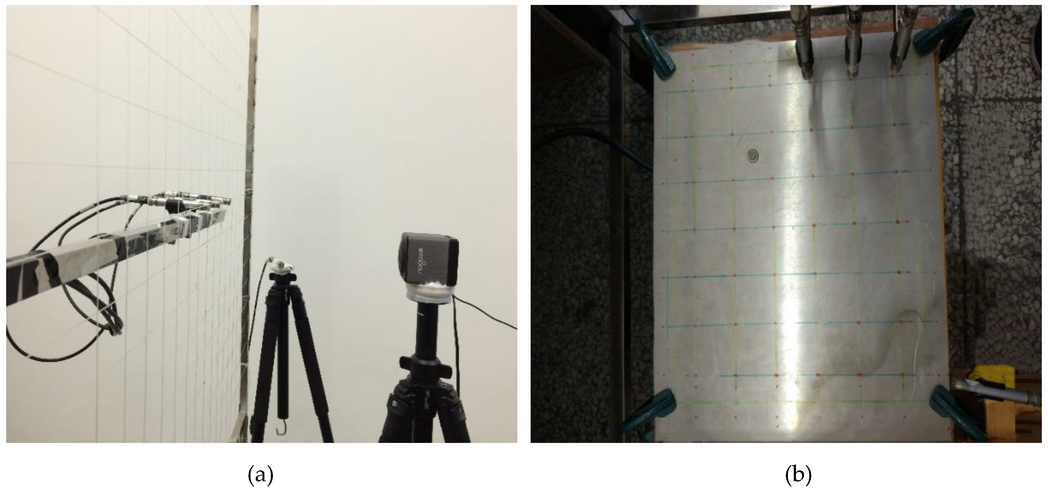
4. Experimental Application

In this section, a couple of experiments including single sound source and plate were carried out to compare the reconstruction performances of the four methods. The experiments were performed in an ordinary room where both sound reflection and random disturbing sources exist. The first experimental setup is shown in Figure 9a. A loudspeaker was used as the sparse sound source. Three microphones with a uniform interspacing of 10 cm were used to measure the pressure on the hologram plane. Another microphone was used as a reference to address the problem that the pressure on all grids points could not be measured simultaneously. The relative phase was preserved by a fixed reference microphone. The pressure was measured on the plane 0.2 m from the loudspeaker with a grid of 6   ×   6 and an interspacing of 10 cm. The reconstruction plane and the equivalent source plane shared the same dimensions of 0.5 m × 0.5 m, a grid of 21   ×   21, and a uniform interspacing of 0.025 m. The two planes were located 0.02 m (reconstruction plane) and 0.001 m (equivalent source plane) from the loudspeaker.
The second experimental setup is shown in Figure 9b. A steel plate with dimensions of 0.35 m ×   0.3 m ×   2 mm was used as the sound source. The plate was fixed by G-type clamps, and it was excited at (0.1 m, 0.1 m) by a vibration exciter. Three microphones with a uniform interspacing of 5 cm were used to measure the pressure on the hologram plane. Another microphone was used as a reference to address the problem that the pressure on all grid points could not be measured simultaneously. The pressure was measured on the plane 5 cm above the plate with a grid of 7   ×   6 and an interspacing of 5 cm. The reconstruction plane and the equivalent source plane shared the same dimensions of 0.3 m   × 0.25 m, a grid of 31 × 26 and a uniform interspacing of 0.01 m. The two planes were located 0.02 m (reconstruction plane) and 0.001 m (equivalent source plane) above the plate. To evaluate the reconstruction, the pressure on the reconstruction plane was also measured to serve as the reference value.
The source maps for a single source based on the four methods are shown in Figure 10. The results showed that for the single source at 500 Hz, it was identified as a large spot in the sound maps of TRESM and CMESM. Compared with the results based on ERDCESM, the resolution of TRESM and CMESM was not satisfactory. For the single source at 2000 Hz, all four methods could detect the position of the target source. However, the accuracy of ERDCESM and CESM was better than that of CMESM and TRESM.
Figure 11 shows contour maps of the reconstructed sound pressure at 500 Hz and 2000 Hz. It shows the results based on ERDCESM- ν on the reconstruction plane. It can be found that all of them identified the peak of the reconstructed sound pressure at the loudspeaker’s location. However, the source map of ERDCESM with order ν = 3 (see Figure 11c and Figure 11f) covered a relatively small area, which demonstrated that it could detect the location of the actual source more accurately. Although there was a position deviation at 500 Hz due to the influence from other interferences, it did not affect the identification of the source localization. Therefore, similar to the simulation, the experimental results also suggested that ERDCESM- ν could identify the source with high accuracy and wide dynamic range.
The reconstructed pressures for plate sound source based on the four methods are shown in Figure 12. It can be seen that for the source at 500 Hz, except TRESM and CESM, the other two methods could reconstruct the sound pressure distribution similar to that of the reference sound pressure. The unsatisfactory reconstruction results of TRESM was mainly due to insufficient measurement points and the influence of environmental noise. At the same time, the main reason for the unsatisfactory effect of CESM was that the basis of CESM was no longer suitable for the spatially extended sound source. Compared with CMESM, ERDCESM had a pressure distribution closer to the referenced. When the plate sound source was set at 2000 Hz, the reconstruction results of the four methods were deviated. This could be explained by the high order acoustic modes possessing high spatial frequency details, which were considered as the evanescent waves in NAH, and were more easily excited when the thickness of the plate was reduced, and thus the sparsity of the sound field was weakened. Another reason was that CS was based on the theory of signal compression, and the evanescent components always had lower weights. Therefore, when the measurement points were not enough, the evanescent components would be discarded. However, it did not affect the identification and location for the area where the radiated sound pressure was the strongest. Compared with the other three methods, ERDCESM realized that the reconstructed strongest radiated sound pressure area was the closest to that of the referenced area.
Figure 13 demonstrates the results based on ERDCESM- ν . It can be seen that with the order ν increasing, the coverage of the identified acoustic center on the reconstruction plane was narrowed gradually and the strongest radiated sound pressure area became more and more obvious. The identification and location for the main noise sources was thus more accurate. Combining the simulation with the application of the experiment, it was found that ERDCESM- v was effective and practical in reconstructing the radiated sound field of the plate.

5. Conclusions

CS is an effective technique rooted on the idea that signal often has a sparse or nearly sparse representation in some bases or dictionaries. However, in many practical applications of acoustics, the characteristics of the source are not clear. It is difficult to find a suitable basis or dictionary for the source. To solve this problem and improve the performance of sound field reconstruction for different types of sources, a compressed ESM based on equivalent redundant dictionary was proposed. In the present work, the following key findings were acquired.
(1) An equivalent redundant dictionary, which combined a series of orthogonal basis U obtained by the SVD method with the equivalent dictionary ϕ used in CESM, was constructed, and it made the proposed method applicable both for sparse and even spatially extended sources.
(2) A reformative method taking advantage of FB, named ERDCESM- v , was developed in this paper. This improved the dynamic range when detecting the source location.
Numerical simulations were performed to compare the reconstructed results of TRESM, CESM, CMESM, and ERDCESM. The results showed that whether the source was distributed sparsely or not sparsely, the reconstruction effect of TRESM was unsatisfactory due to the insufficient measurement points. When the source was distributed sparsely, CESM achieved the best reconstruction effect, and the accuracy of ERDCESM was almost as good as that of CESM. When the source was not distributed sparsely (e.g., the spatially extended source), both CMESM and ERDCESM had higher reconstruction accuracy than TRESM and CESM. However, compared with CMESM, ERDCESM could provide more accurate results since the dictionary of ERDCESM was complex-valued and contained more phase information. Therefore, ERDCESM produced a satisfactory reconstruction result, which indicated that it was more flexible for different types of sources. By combining the advantages of FB, ERDCESM- v could provide more a accurate source position (for the spatially sparse source) or locate the strongest radiated sound pressure area (for the spatially extended source).
The proposed method was also tested by experimental applications. The results indicated that the proposed method was practical and reliable for different types of sound sources.

Author Contributions

Investigation, Y.H.; Writing—original draft, Y. H.; Methodology, Y.H and L.C.; Software. L.C.; Data curation, L.C.; Writing—review and editing, Y.H. and L.C.; Project administration, Z.X. and Z.Z.; Resources, Z.X. and Z.Z.

Funding

This research received no external funding.

Acknowledgments

This work was supported by the Natural Science Foundation of China (Grant No. 11874096) and the Fundamental Research Funds for the Central Universities (Project No. 106112016CDJXZ338825). These projects covered all the costs of this series of research. The authors appreciate their support in this research.

Conflicts of Interest

The authors declare no conflict of interest.

Nomenclature

SymbolDescription
p ( m ) Sound pressure at the m-th point
g ( r m | r n ) The pressure transfer function linking the n -thequivalent source to the m -th microphone
k Acoustic wavenumber, rad/m
|| r m n || The distance between the considered source microphone couple
A The transfer matrix relating the measured pressures to the equivalent sources
ω Angular frequency, rad/s
ρ Density, kg/m3
p Measured sound pressure
q Source strength vector
Γ λ ( q ) Cost function
λ Regularization parameter
P R Sound pressure on the reconstruction plane
G The transfer matrix relating the reconstruction points to the equivalent sources
I Identity matrix
α Coefficient vector of the basis
ϕ Equivalent dictionary
U Unitary matrix
V Unitary matrix
H Conjugate transpose
S Real diagonal matrix
λ i Singular values
β Coefficient vector of the basis
D Equivalent redundant dictionary
+ Moore–Penrose inverse
ε Tolerance
σ A small number
Υ Coefficient vector
C Cross spectral matrix
v Order
Z i Sound pressure at the   i -th point on the reconstruction plane
P t Theoretical pressure
P r Reconstructed pressure

References

  1. Koopmann, G.H.; Song, L.; Fahnline, J.B. A method for computing acoustic fields based on the principle of wave superposition. J. Acoust. Soc. Am. 1989, 86, 2433–2438. [Google Scholar] [CrossRef]
  2. Sarkissian, A. Method of superposition applied to patch near-field acoustic holography. J. Acoust. Soc. Am. 2005, 118, 671–678. [Google Scholar] [CrossRef]
  3. Valdivia, N.P.; Williams, E.G. Study of the comparsion of the methods of equivalent sources and boundary element methods for near-field acoustic holography. J. Acoust. Soc. Am. 2006, 120, 3694–3705. [Google Scholar] [CrossRef] [PubMed]
  4. Ping, G.; Chu, Z.; Xu, Z.; Shen, L. A refined wideband acoustical holography based on equivalent source method. Sci. Rep. 2017, 7, 43458. [Google Scholar] [CrossRef] [PubMed] [Green Version]
  5. Zhongming, X.; Qinghua, W.; Yansong, H.; Zhifei, Z.; Shu, L.; Mengran, L. A monotonic two-step iterative shrinkage/thresholding algorithm for sound source identification based on equivalent source method. Appl. Acoust. 2018, 129, 386–396. [Google Scholar] [CrossRef]
  6. Xu, C.; Mao, Y.J.; Hu, Z.W. Improved Equivalent Source Method to Predict Sound Scattered by Solid Surfaces. AIAA J. 2018, 57, 513–520. [Google Scholar] [CrossRef]
  7. Bai, M.R. Application of BEM (boundary element method)-based acoustic holography to radiation analysis of sound sources with arbitrarily shaped geometries. J. Acoust. Soc. Am. 1992, 92, 533–549. [Google Scholar] [CrossRef]
  8. Wu, S.F.; Yu, J. Reconstructing interior acoustic pressure field via Helmholtz equation least-squares method. J. Acoust. Soc. Am. 1998, 104, 2054–2060. [Google Scholar] [CrossRef]
  9. Hald, J. Basic theory and properties of statistically optimized near-field acoustical holography. J. Acoust. Soc. Am. 2009, 125, 2105–2120. [Google Scholar] [CrossRef] [PubMed]
  10. Antoni, J. A Bayesian approach to sound source reconstruction: Optimal basis, regularization, and focusing. J. Acoust. Soc. Am. 2012, 131, 2873–2890. [Google Scholar] [CrossRef] [PubMed]
  11. Leclere, Q. Acoustic imaging using under-determined inverse approaches: Frequency limitations and optimal regularization. J. Sound Vib. 2009, 321, 605–619. [Google Scholar] [CrossRef]
  12. Bai, M.R.; Chung, C.; Wu, P.C. Solution strategies for linear inverse problems in spatial audio signal processing. Appl. Sci. 2017, 7, 582. [Google Scholar] [CrossRef]
  13. Gao, B.; Xiao, S.; Zhao, L. Convergence Gain in Compressive Deconvolution: Application to Medical Ultrasound Imaging. Appl. Sci. 2018, 8, 2558. [Google Scholar] [CrossRef]
  14. Jin, W.; Kleijn, W.B. Theory and design of multizone sound field reproduction using sparse methods. IEEE/ACM Trans. Audio Speech Lang. Process. 2015, 23, 2343–2355. [Google Scholar]
  15. Candes, E.J.; Wakin, M.B. An introduction to compressive sampling. IEEE Signal Proc. Mag. 2008, 25, 21–30. [Google Scholar] [CrossRef]
  16. Chardon, G.; Daudet, L.; Peillot, A.; Bertin, N. Near-field acoustic holography using sparse regularization and compressive sampling principles. J. Acoust. Soc. Am. 2012, 132, 1521–1534. [Google Scholar] [CrossRef] [PubMed]
  17. Fernandez-Grande, E.; Xenaki, A. Compressive sensing with a spherical microphone array. J. Acoust. Soc. Am. 2016, 139, 45–49. [Google Scholar] [CrossRef] [PubMed]
  18. Fernandez-Grande, E.; Daudet, L. A sparse equivalent source method for near-field acoustic holography. J. Acoust. Soc. Am. 2017, 141, 532–542. [Google Scholar] [CrossRef] [PubMed]
  19. Hald, J. Wideband acoustical holography. In Proceedings of the Inter-Noise 2014, Melbourne, Australia, 16–19 November 2014. [Google Scholar]
  20. Hald, J. Fast wideband acoustical holography. J. Acoust. Soc. Am. 2016, 139, 1508–1517. [Google Scholar] [CrossRef] [PubMed]
  21. Fernandez-Grande, E.; Xenaki, A. The equivalent source method as a sparse signal reconstruction. In Proceedings of the Inter-Noise 2015, San Francisco, CA, USA, 9–12 August 2015. [Google Scholar]
  22. Fernandez-Grande, E.; Daudet, L. Near-field acoustic imaging based on Laplacian sparsity. In Proceedings of the 22nd International Congress on Acoustic, Buenos Aires, Argentina, 5–9 September 2016. [Google Scholar]
  23. Bi, C.X.; Liu, Y.; Xu, L.; Zhang, Y.B. Sound field reconstruction using compressed modal equivalent point source method. J. Acoust. Soc. Am. 2017, 141, 73–79. [Google Scholar] [CrossRef] [PubMed]
  24. Li, S.; Xu, Z.; He, Y.; Zhang, Z.; Song, S. Functional Generalized Inverse Beamforming Based on the Double-Layer Microphone Array Applied to Separate the Sound Sources. ASME J. Vib. Acoust. 2016, 138, 021013. [Google Scholar] [CrossRef]
  25. Harker, B.M.; Gee, K.L.; Neilsen, T.B.; Wall, A.T. Comparison of beamforming methods to reconstruct extended, partially-correlated sources. J. Acoust Soc. Am. 2017, 141, 3984. [Google Scholar] [CrossRef]
  26. Oudompheng, B.; Pereira, A.; Picard, C.; Leclere, Q.; Nicolas, B. A Theoretical and Experimental Comparison of the Iterative Equivalent Source Method and the Generalized Inverse Beamforming. In Proceedings of the Berlin Beamforming Conference, Berlin, Germany, 19–20 February 2014; pp. 1273–1282. [Google Scholar]
  27. Photiadis, D.M. The relationship of singular value decomposition to wave vector filtering in sound radiation problems. J. Acoust. Soc. Am. 1990, 88, 1152–1159. [Google Scholar] [CrossRef]
  28. Hu, D.Y.; Li, H.B.; Hu, Y.; Fang, Y. Sound field reconstruction with sparse sampling and the equivalent source method. Mech. Syst. Signal Process. 2018, 108, 317–325. [Google Scholar] [CrossRef]
  29. Williams, E.G.; Houston, B.H.; Herdic, P.C. Fast Fourier transform and singular value decomposition formulations for patch nearfield acoustical holography. J. Acoust. Soc. Am. 2003, 114, 1322–1333. [Google Scholar] [CrossRef] [PubMed]
  30. Cannistraro, G.; Cannistraro, M.; Cannistraro, A. Evaluation of the Sound Emission and Climate Acoustic in Proximity of one Railway Station. IJH T 2016, 34, S589–S596. [Google Scholar]
  31. Cannistraro, M.; Chao, J.; Ponterio, L. Experimental study of air pollution in the urban centre of the city of Messina. Model. Meas. Control C 2018, 79, 133–139. [Google Scholar] [CrossRef]
  32. Grant, M.; Boyd, S. CVX: MATLAB Software for Disciplined Convex Programming, Version 2.1. Available online: http://cvxr.com/cvx (accessed on 10 December 2018).
Figure 1. The diagrammatic sketch of the equivalent source method (ESM).
Applsci 09 00808 g001
Figure 2. The array with 64 randomly distributed microphones.
Applsci 09 00808 g002
Figure 3. Reconstructed error for a single sound source. Frequency interval is 50 Hz.
Applsci 09 00808 g003
Figure 4. The calculated sound maps of (a) Theoretical map at 500 Hz, (b) TRESM map at 500 Hz, (c) CESM map at 500 Hz, (d) CMESM map at 500 Hz, (e) ERDCESM map at 500 Hz, (f) Theoretical map at 2000 Hz, (g) TRESM map at 2000 Hz, (h) CESM map at 2000 Hz, (i) CMESM map at 2000 Hz and (j) ERDCESM map at 2000 Hz for a single source.
Applsci 09 00808 g004
Figure 5. Pressure distributions of (a) the sound pressure at 500 Hz, (b) ERDCESM with ν = 0 at 500 Hz, (c) ERDCESM with ν = 1 at 500 Hz, (d) ERDCESM with ν = 3 at 500 Hz, (e) the sound pressure at 2000 Hz, (f) ERDCESM with ν = 0 at 2000 Hz, (g) ERDCESM with ν = 1 at 2000 Hz and (h) ERDCESM with ν = 3 at 2000 Hz for a single source.
Applsci 09 00808 g005
Figure 6. Reconstructed error for a simply supported plate. Frequency interval is 50 Hz.
Applsci 09 00808 g006
Figure 7. The calculated sound maps of (a) Theoretical map at 500 Hz, (b) TRESM map at 500 Hz, (c) CESM map at 500 Hz, (d) CMESM map at 500 Hz, (e) ERDCESM map at 500 Hz, (f) Theoretical map at 2000 Hz, (g) TRESM map at 2000 Hz, (h) CESM map at 2000 Hz, (i) CMESM map at 2000 Hz and (j) ERDCESM map at 2000 Hz for a simply supported plate.
Applsci 09 00808 g007
Figure 8. Pressure distributions of (a) ERDCESM with ν = 0 , (b) ERDCESM with ν = 1 , (c) ERDCESM with ν = 3 and (d) ERDCESM with ν = 5 for a simply supported plate at 500 Hz.
Applsci 09 00808 g008
Figure 9. Experimental setup: (a) Single source; (b) Plate sound source.
Applsci 09 00808 g009
Figure 10. The Experimental results of (a) TRESM map at 500 Hz, (b) CESM map at 500 Hz, (c) CMESM map at 500 Hz, (d) ERDCESM map at 500 Hz, (e) TRESM map at 2000 Hz, (f) CESM map at 2000 Hz, (g) CMESM map at 2000 Hz and (h) ERDCESM map at 2000 Hz for a single source.
Applsci 09 00808 g010
Figure 11. Pressure distributions under experimental conditions of (a) ERDCESM with ν = 0 at 500 Hz, (b) ERDCESM with ν = 1 at 500 Hz, (c) ERDCESM with ν = 3 at 500 Hz, (d) ERDCESM with ν = 0 at 2000 Hz, (e) ERDCESM with ν = 1 at 2000 Hz and (f) ERDCESM with ν = 3 at 2000 Hz for a single source.
Applsci 09 00808 g011
Figure 12. The Experimental results of (a) Theoretical map at 500 Hz, (b) TRESM map at 500 Hz, (c) CESM map at 500 Hz, (d) CMESM map at 500 Hz, (e) ERDCESM map at 500 Hz, (f) Theoretical map at 2000 Hz, (g) TRESM map at 2000 Hz, (h) CESM map at 2000 Hz, (i) CMESM map at 2000 Hz and (j) ERDCESM map at 2000 Hz for a plate sound source.
Applsci 09 00808 g012
Figure 13. Pressure distributions under experimental conditions of (a) ERDCESM with ν = 0 , (b) ERDCESM with ν = 1 , (c) ERDCESM with ν = 3 and (d) ERDCESM with ν = 5 for a plate sound source at 500 Hz.
Applsci 09 00808 g013

