Day-Ahead Optimal Battery Operation in Islanded Hybrid Energy Systems and Its Impact on Greenhouse Gas Emissions

Abstract

This paper proposes a management strategy for the daily operation of an isolated hybrid energy system (HES) using heuristic techniques. Incorporation of heuristic techniques to the optimal scheduling in day-head basis allows us to consider the complex characteristics of a specific battery energy storage system (BESS) and the associated electronic converter efficiency. The proposed approach can determine the discharging time to perform the load peak-shaving in an appropriate manner. A recently proposed version of binary particle swarm optimization (BPSO), which incorporates a time-varying mirrored S-shaped (TVMS) transfer function, is proposed for day-ahead scheduling determination. Day-ahead operation and greenhouse gas (GHG) emissions are studied through different operating conditions. The complexity of the optimization problem depends on the available wind resource and its relationship with load profile. In this regard, TVMS-BPSO has important capabilities for global exploration and local exploitation, which makes it a powerful technique able to provide a high-quality solution comparable to that obtained from a genetic algorithm.

1. Introduction

Global warming and other environmental problems are driving the adoption of renewable energy sources at the residential, commercial, and industrial levels. Estimating the impact of climate change on the ecosystem involves the accurate knowledge of the carbon cycle and its associated uncertainty. Calculating cumulative emissions in order to prevent an extreme warming level is a key step to guide the manner in which industrial processes, including power generation, should be carried out. Actions for reducing global warming are adjusted following the threshold of 1.5 or 2 °C as the critical limit in a time interval between the years 2000 and 2050 or 2100. However, depending on the established assumptions and scenarios, the risk of experiencing extreme conditions at the middle of the century could be a realistic prospect [1].

Under these circumstances, many countries have been changing their energy mix from a fossil-fuel based one to a renewable-based one, incorporating wind and solar photovoltaic energies, as well as demand response programs [2]. In addition, financial tools such as mutual funds are also implemented to provide economic support for these technologies [3].

As renewable energies are intrinsically variable, the power system requires a high degree of flexibility to effectively manage the uncertainty introduced by these sources, and this could be achieved by implementing demand side management or by installing any type of energy storage system (ESS).

Incorporation of ESS can improve the accommodation of renewable generation while reducing greenhouse gas (GHG) emissions. As an example, incorporation of renewable power combined with ESS in California could reduce carbon dioxide (CO₂) emissions from 90% to 72%, whereas renewable power curtailment reduces from 33% to 9%. In the case of Texas, CO₂ emissions could be reduced from 58% to 54% and renewable power curtailment could be reduced from 3% to 0.3% [4]. Combination of carbon capture and storage devices with conventional generation units is also an option to reduce GHG emissions. However, the combination of renewable generation with ESS can be energetically more effective [5].

Historically, the acquisition costs of a battery energy storage system (BESS) have been considerably high, limiting their economic performance and consequently their mass adoption. However, when very low GHG emissions are required, BESS can be a critical device to achieve such an ambitious goal.

In the case of energy provision for an isolated hybrid energy system (HES), incorporation of BESS becomes profitable due to the fact that the fuel consumption and operating hours of a conventional generator are considerably reduced. In the case of a grid-connected HES, retailing rates and feed-in tariffs as well as favorable resources are crucial for their successful adoption [6].

Heuristic techniques are commonly used to carry out the optimal sizing of a specific HES. Consequently, some of them have been implemented in computational programs such as HOMER Pro^® [7], iHOGA^® [8], and Hybrid2^® [9], among others. Dispatch strategies implemented in most of these tools are based on load following and cycle charging concepts. Load following consists of generating power from conventional units only to satisfy net load (NL), and this approach is frequently suggested in a HES with high share of renewable power, which is much higher than load demand over the year. Conversely, a cycle charging strategy forces conventional generator to operate at its rating power when needed to charge BESS with the remaining energy, so this strategy is frequently implemented when renewable generation is limited [10]. It is important to mention that these strategies do not require any forecast of renewable generation or load demand. However, they are very effective in the management of HES of small scale used on rural electrification projects.

In the case of a HES of larger scale, energy forecasts are frequently employed to optimize the daily operation. This is a topic that has been widely studied and it is the focus of this work. A complete literature review is presented in the next section.

1.1. Literature Review

Management of isolated HES considering the influence of renewable resources and their associated variability has been treated by many authors. In this regard, Li et al. [11] developed a procedure for sizing and management of wind–BESS units. Historical wind power time series is analyzed to estimate the low-frequency component, which is the most prominent one. Using the resulting signal, charging–discharging cycles of BESS are determined considering constant power levels. During the charging period, the power to be provided by the wind–BESS unit is set to the minimum power of low-frequency component within that period. Conversely, power generation is scheduled to the highest power of low-frequency component during discharging periods. In theory, these mechanisms ensure the existence of sequential charging–discharging intervals. However, power dispatch settings could be modified to avoid the charging–discharging cycles at partial level. Other issues related to the wind power forecasting error and BESS lifetime have also been incorporated.

Luo et al. [12] created a model for the operation and sizing of wind–BESS to compensate for the forecasting error. Forecasting error is modeled by using a beta distribution, considering extreme conditions related to pessimistic and optimistic perspectives. BESS dynamic behavior, as well as its lifetime, have been also incorporated.

Mohammadi et al. [13] proposed a day-ahead scheduling model of a microgrid (MG) composed of electrical as well as hydrogen and thermal energy storage technologies. Problem formulation was based on a two-stage stochastic programming approach, while its solution was carried out using an enhanced version of cuckoo optimization algorithm. The high flexibility of the studied configuration results is useful to deal with the fact that thermal and electrical energy consumption are typically not synchronized.

O’Dwyer and Flynn [14] paid special attention to the power system operation on a daily basis, using hourly and sub-hourly time steps, under high renewable energy integration and ESS. According to the reported results, the traditional hourly analysis cannot properly estimate the ramping requirements, the number of starts of conventional generators, as well as the role and potential of ESS on the cycling reduction. Consequently, the interdependence between renewable power curtailment, CO₂ emissions, and the cycling process of thermal units is not accurately described.

Wen et al. [15] presented an enhanced security-constrained unit commitment (SCUC) model, which incorporates BESS to mitigate the negative effects of a sudden contingency and consequently to prevent cascading outages. The methodology was formulated as a two-stage mixed integer programming problem and solved by means of Benders decomposition. The same author in [16] introduced a model based on frequency dynamic constrained unit commitment (UC) able to incorporate wind power uncertainty. Interval optimization approach was combined with mixed integer linear programming (MILP) to determine the appropriate unit schedule.

Nguyen and Crow [17] presented a scheduling model with probabilistic constraints based on stochastic dynamic programming (DP). The proposed BESS-model is inspired by the functioning of conventional fuel-based units. Thus, a detailed cost model was developed considering the electrochemical process of BESS.

Khorramdel et al. [18] proposed a UC model based on cost-benefit analysis, in which a probabilistic analysis based on a here-and-now approach was incorporated. Then, particle swarm optimization (PSO) was implemented in order to minimize total generating costs.

Li et al. [19] developed a framework to quantify the benefits of ESS incorporation to HES. The methodology is based on stochastic UC solved by means of MILP.

Jiang et al. [20] proposed a management model for a residential HES provided by wind generation, micro-combined heat and power generation and smart appliances, enrolled in a real-time pricing (RTP) program. Additionally, optimal behavior of several aggregated HESs is analyzed by means of a day-ahead stochastic economic dispatch (ED) and UC model based on MILP.

Anand and Ramasubbu [21] presented a scheduling model of a system enrolled in a RTP program composed of wind and photovoltaic generation, as well as a microturbine and a fuel cell, based on anti-predatory PSO.

Wu et al. [22] proposed a methodology to solve ED and UC problems using the time-scaling transformation combined with an auxiliary continuous vector.

Dui et al. [23] proposed a two-stage scheduling methodology for BESS performance evaluation. In the first step, UC problem including the effects of thermal and wind generators is solved by means of second-order cone programming. Then, in the second step, the management strategy for BESS is designed and evaluated using a genetic algorithm (GA).

Psarros et al. [24] investigated the operation of HESs using a MILP. BESS sizing is deeply discussed, concluding that this element is a key device for the provision of fast energy reserve. The same author in [25] proposed a model able to consider different time resolutions, based on the combination of model predictive control and MILP.

Ahmadi et al. [26] presented a model for the solution of SCUC including BESS. Aging cost related to BESS operation is incorporated to the objective function. Then, MILP is combined with information-gap decision theory so that the conservatism of the strategy to be implemented can be adjusted by the system operator.

Saleh [27] created and experimentally tested the performance of an energy management system (EMS) based on the solution of UC by Lagrangian relaxation. Thus, control values of permanent magnet generator of the wind turbine and the power-electronic converter are obtained.

Gupta et al. [28] formulated a SCUC model including the effects of BESS in order to compensate the variability of renewable power sources. The mathematical problem is solved by using Benders decomposition, determining the locational marginal price, wind power curtailment, as well as the line contingency.

Alvarez et al. [29] proposed a general purpose ESS model inspired by the behavior of hydraulic reservoirs. Using the results obtained from stochastic dual DP, carried out to determine the long-term energy schedule, the linear model of ESS cost is derived. Finally, stochastic UC, including the aforementioned ESS model, was formulated.

Chen et al. [30] developed a scheduling model based on multi-agent system for the coordination of multiple MGs. Such coordination is carried out by means of the alternating direction method of multipliers, obtaining the optimal energy management of the multiple MGs. Additionally, the negative effects of uncertainty sources are compensated by using day-in rolling.

Tan et al. [31] proposed a dispatch model able to incorporate different operating perspectives related to fuel savings, carbon emissions, power generation costs, amount of renewable energy integrated, and power generation efficiency. Uncertainty of renewable generation and forecasting of carbon-trading price were included by using Monte Carlo simulations, while the associated optimization model was solved by implementing the technique for order preference by similarity to ideal solution combined with Grey relational analysis.

Yiwei et al. [32] presented a scheduling model for a HES based on renewable and thermal generation, as well as cascade hydropower and pumped ESS. The model focuses on the economy and security aspects of system operation. The optimization strategy is divided into three main stages. During the first stage, integer variables are preprocessed using heuristic rules. Then, during the second stage, ED and UC are solved. Finally, during stage three, power system feasibility was evaluated.

Once the literature review has been exposed, describing the state-of-the-art techniques used for day-ahead scheduling, the main contribution and novelty of this work are carefully explained in the next section.

1.2. Main Contributions

As can be observed from the presented literature review, a vast family of methodologies has been created, some of them based on heuristic techniques such as GA and PSO, another group inspired by DP, and most of them based on MILP combined with Benders decomposition.

In a general sense, the optimization technique to be selected strongly depends on the characteristics and assumptions of the ESS model, as well as the context (isolated or grid-connected system) and the information available.

To take advantage of the vast family of BESS models, a recently developed version of binary PSO (BPSO), which incorporates a time-varying mirrored S-shaped (TVMS) transfer function, has been adopted in this paper. Consequently, hourly behavior of charging–discharging efficiency as well as the influence of charge controller on battery operation can be effectively incorporated. Additionally, the influence of wind-speed daily profile on battery schedule and GHG emissions is deeply analyzed. The impact of battery operation on the emissions of total hydrocarbons (THC), carbon monoxide (CO), oxides of nitrogen (NO_X), CO₂, and particulate matter (PM) is investigated.

The remainder of the paper is organized as follows. Section 2 describes the mathematical models of the system configuration under study. Section 3 explains the formulation of the optimization problem and its solution by TVMS-BPSO. Then, problem formulation is tested in Section 4 through a sensitivity analysis based on GA. As TVMS-BPSO is a novel version of BPSO, its performance is compared with GA in Section 5. Finally, conclusions and main findings are discussed in Section 6.

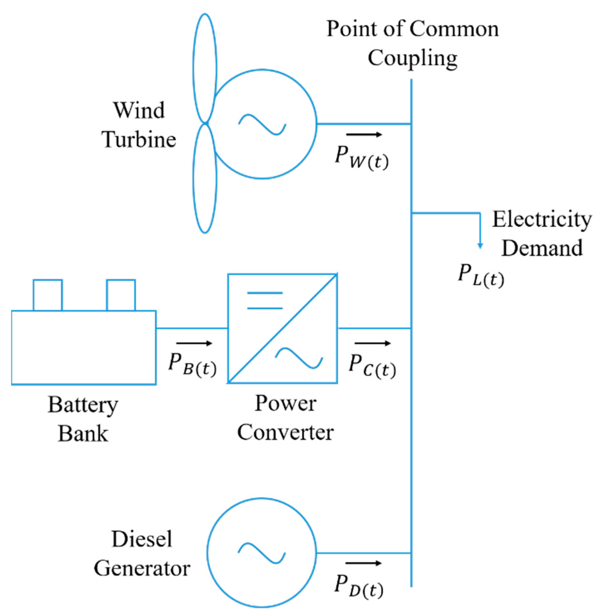
2. Hybrid Energy System Model

The structure of the HES under analysis is shown in Figure 1. On one hand, the diesel generator represents the controllable power source able to provide energy under any circumstance. Thus, energy not supplied (ENS) is neglected. Due to the fact that the diesel generator has important operating costs related to fuel consumption and overhauling, the incorporation of the wind generator combined with BESS and power converter allows us to reduce the number of operating hours of the diesel unit, reducing the operating costs of the whole system.

Besides the wind generator, BESS, power converter, and diesel generator, the dump load (not shown in Figure 1) allows us to consume all the energy surplus of the system in order to maintain the energy balance. This could occur when BESS reaches its maximum capacity and a high magnitude of wind power is available.

In the next sections, computational models of the wind generator, BESS, and diesel generator will be carefully described.

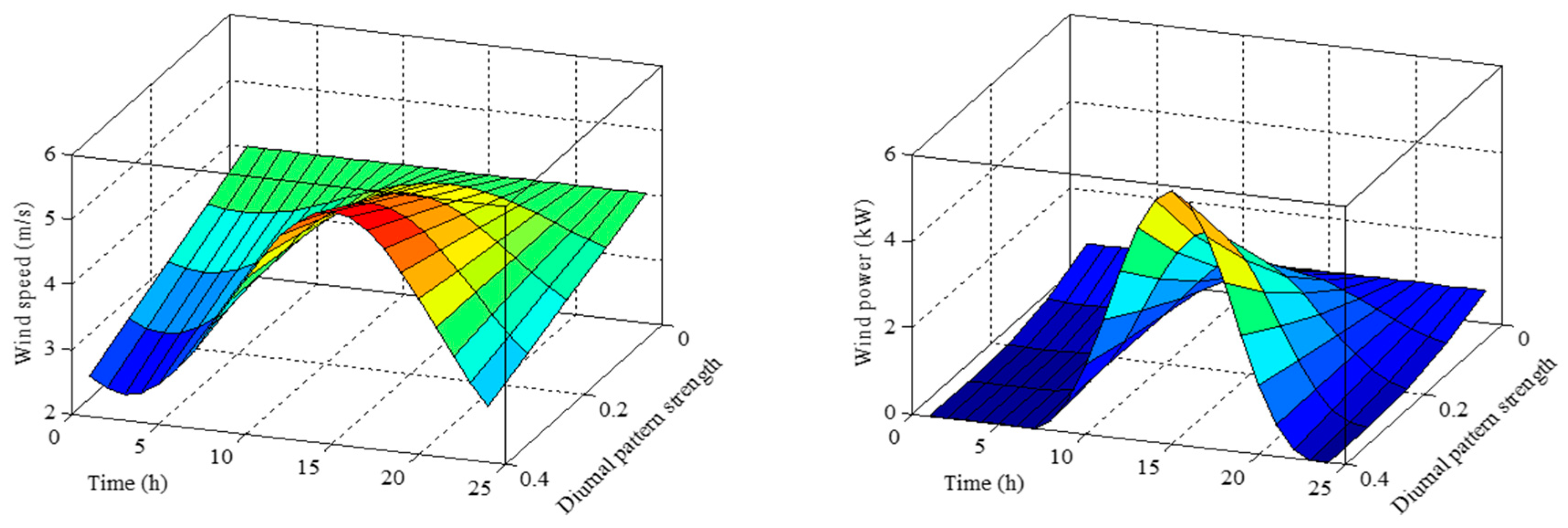
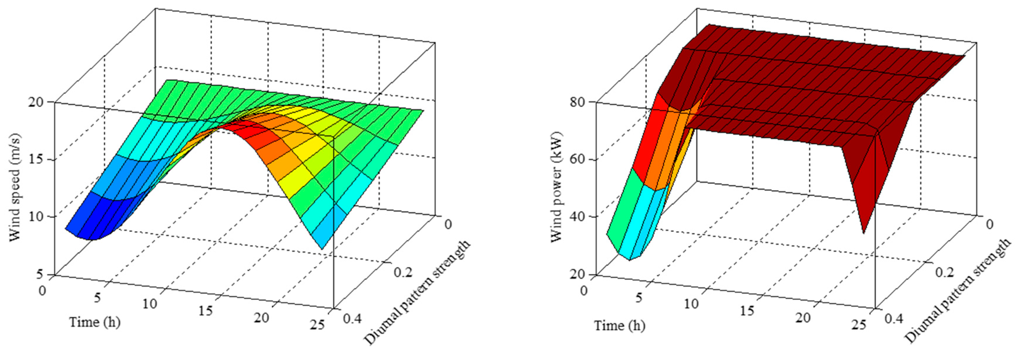
2.1. Wind Generator Model

Wind power generation has been modeled using a typical power curve described according to Equations (1)–(4) [33,34]:

$$P_{W\left(t\right)}=\{\begin{array}{c}0; 0\le S_{W\left(t\right)}\le S_W^o\\ P_W^a+P_W^b\left(S_{W\left(t\right)}\right)+P_W^c{\left(S_{W\left(t\right)}\right)}^2; S_W^o\le S_{W\left(t\right)}\le S_W^r\\ \begin{array}{c}{P}_W^{max}; S_W^r\le S_{W\left(t\right)}\le S_W^f\\ 0; S_{W\left(t\right)}>S_W^f\end{array}\end{array} \forall t=1,\dots ,T;$$

(1)

$$P_W^a=\frac{1}{{\left(S_W^o-S_W^r\right)}^2}\left[S_W^o\left(S_W^o+S_W^r\right)-4S_W^o{S}_W^r{\left(\frac{S_W^o+S_W^r}{2S_W^r}\right)}^3\right];$$

(2)

$$P_W^b=\frac{1}{{\left(S_W^o-S_W^r\right)}^2}\left[4\left(S_W^o+S_W^r\right){\left(\frac{S_W^o+S_W^r}{2S_W^r}\right)}^3-\left(3S_W^o+S_W^r\right)\right];$$

(3)

$$P_W^c=\frac{1}{{\left(S_W^o-S_W^r\right)}^2}\left[2-4{\left(\frac{S_W^o+S_W^r}{2S_W^r}\right)}^3\right];$$

(4)

In this way, the relationship between the wind speed ($S_{W\left(t\right)}$) at a determined time step ($t$) and the corresponding wind power production ($P_{W\left(t\right)}$) is clearly established.

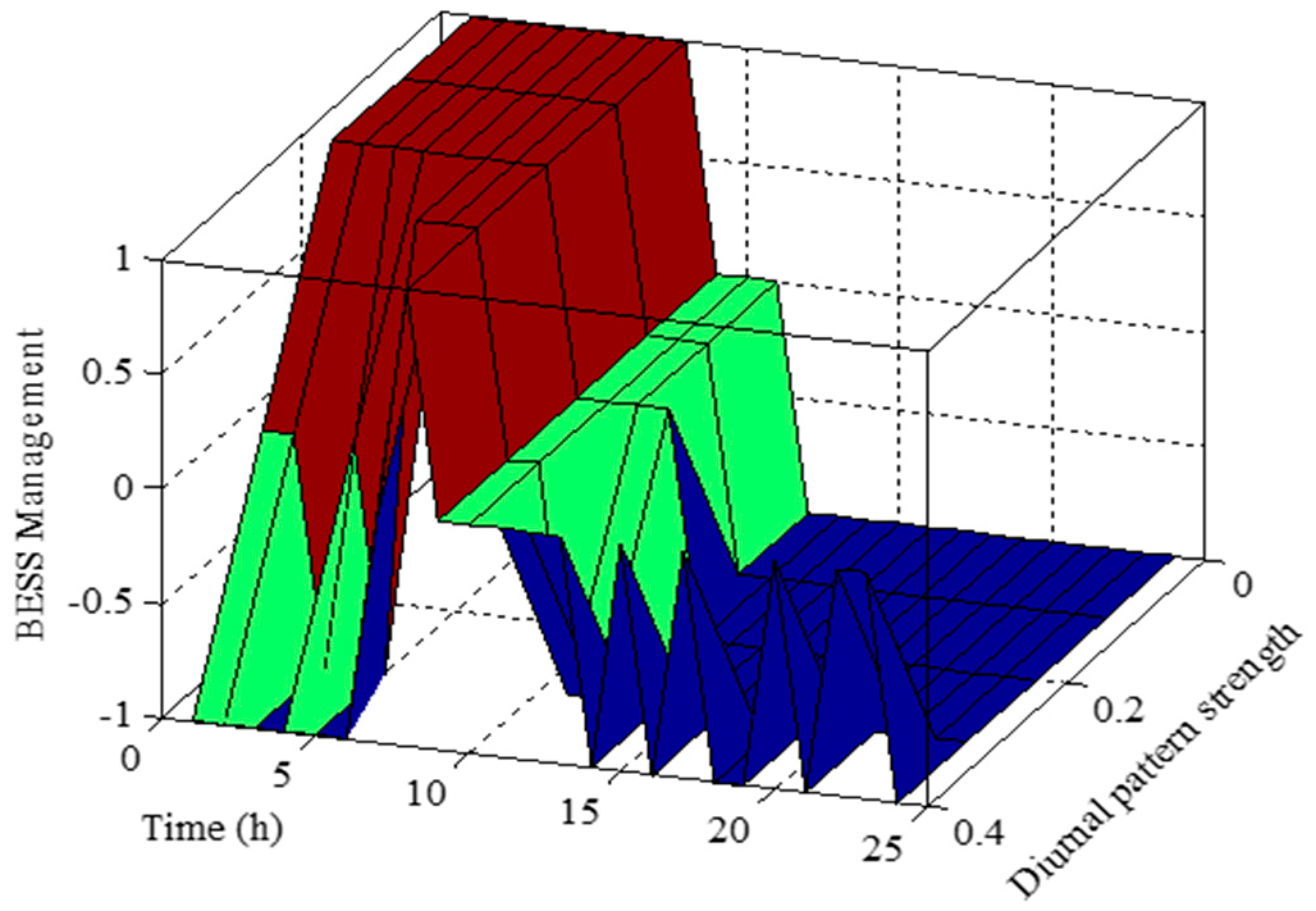
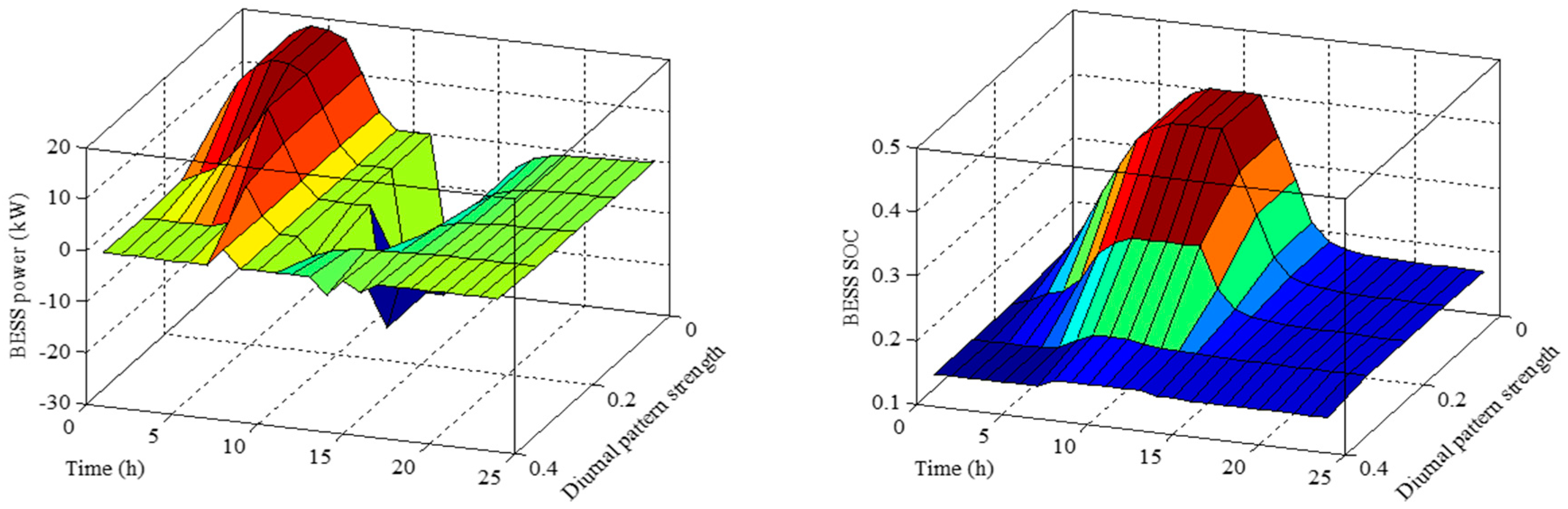
2.2. BESS and Power Converter Models

BESS is a crucial device for the appropriate operation of HES because it provides operational flexibility to the whole system. The technology chosen in this work is the vanadium redox flow battery (VRFB) due to its easy scalability, which makes it appropriate for large-scale integration. The mathematical model adopted is shown in Equations (5)–(15), and it has been experimentally tested and validated in [35,36,37].

Battery voltage ($U_{B\left(t\right)}$) and efficiency (${\eta }_{B\left(t\right)}$) are defined according to charging and discharging processes using Equations (5) and (6), respectively.

$$U_{B\left(t\right)}=\{\begin{array}{c}{U}_{B\left(t\right)}^{ch}; P_{B\left(t\right)}>0\\ U_{B\left(t\right)}^{dis}; P_{B\left(t\right)}\le 0 \end{array}\forall t=1,\dots ,T;$$

(5)

$${\eta }_{B\left(t\right)}=\{\begin{array}{c}{\eta }_{B\left(t\right)}^{ch}; P_{B\left(t\right)}>0\\ {\eta }_{B\left(t\right)}^{dis}; P_{B\left(t\right)}<0\end{array} \forall t=1,\dots ,T.$$

(6)

During charging process, when battery power ($P_{B\left(t\right)}$) is positive, battery voltage ($U_{B\left(t\right)}^{ch}$) is related to the state of charge (SOC) ($SO{C}_{B\left(t\right)}$) according to (7), while charging efficiency for voltage (${\eta }_{V\left(t\right)}^{ch}$) and energy (${\eta }_{E\left(t\right)}^{ch}$) are related to SOC and battery power as shown in (8) and (9), respectively. Then, global efficiency of charging phenomena (${\eta }_{B\left(t\right)}^{ch}$) can be estimated using (10).

$$U_{B\left(t\right)}^{ch}=\left(U_{ch}^{a}SO{C}_{B\left(t\right)}+U_{ch}^b\right)P_{B\left(t\right)}+U_{ch}^{c}SO{C}_{B\left(t\right)}+U_{ch}^d \forall t=1,\dots ,T;$$

(7)

$${\eta }_{V\left(t\right)}^{ch}=\frac{U_{ch}^e{T}_E\left(SO{C}_{B\left(t\right)}-U_{ch}^f\right)+U_{ch}^g}{\left(U_{ch}^{h}SO{C}_{B\left(t\right)}+U_{ch}^j\right)P_{B\left(t\right)}+U_{ch}^{k}SO{C}_{B\left(t\right)}+U_{ch}^l} \forall t=1,\dots ,T;$$

(8)

$${\eta }_{E\left(t\right)}^{ch}=\frac{\left(U_{ch}^{m}SO{C}_{B\left(t\right)}+U_{ch}^n\right)P_{B\left(t\right)}+U_{ch}^{p}SO{C}_{B\left(t\right)}-U_{ch}^q}{P_{B\left(t\right)}} \forall t=1,\dots ,T;$$

(9)

$${\eta }_{B\left(t\right)}^{ch}={\eta }_{V\left(t\right)}^{ch}{\eta }_{E\left(t\right)}^{ch} \forall t=1,\dots ,T.$$

(10)

During discharging process ($P_{B\left(t\right)}<0$), battery voltage ($U_{B\left(t\right)}^{dis}$) and SOC are related according to the linear expression shown in (11). Voltage and energy efficiencies (${\eta }_{V\left(t\right)}^{dis}$ and ${\eta }_{E\left(t\right)}^{dis}$) depend on battery power and SOC following (12) and (13), respectively. Thus, discharging efficiency (${\eta }_{B\left(t\right)}^{dis}$) is estimated through the product of these variables (${\eta }_{V\left(t\right)}^{dis}$ and ${\eta }_{E\left(t\right)}^{dis}$), as suggested in (14).

$$U_{B\left(t\right)}^{dis}=U_{dis}^a\left|P_{B\left(t\right)}\right|+U_{dis}^{b}SO{C}_{B\left(t\right)}+U_{dis}^c \forall t=1,\dots ,T;$$

(11)

$${\eta }_{V\left(t\right)}^{dis}=\frac{U_{dis}^d\left|P_{B\left(t\right)}\right|+U_{dis}^{e}SO{C}_{B\left(t\right)}+U_{dis}^f}{U_{dis}^g{T}_E\left(SO{C}_{B\left(t\right)}-U_{dis}^h\right)+U_{dis}^j} \forall t=1,\dots ,T;$$

(12)

$${\eta }_{E\left(t\right)}^{dis}=\frac{\left|P_{B\left(t\right)}\right|}{U_{dis}^k\left|P_{B\left(t\right)}\right|+U_{dis}^{l}SO{C}_{B\left(t\right)}\left(SO{C}_{B\left(t\right)}-1\right)+U_{dis}^m} \forall t=1,\dots ,T;$$

(13)

$${\eta }_{B\left(t\right)}^{dis}={\eta }_{V\left(t\right)}^{dis}{\eta }_{E\left(t\right)}^{dis} \forall t=1,\dots ,T.$$

(14)

SOC at a determined time interval ($t$) is defined using (15), which depends on the battery power and efficiency, calculated by following the equations previously described.

$$SO{C}_{B\left(t\right)}=SO{C}_{B\left(t-1\right)}+\underset{t-1}{\overset{t}{{\displaystyle \int }}}\left(\frac{P_{B\left(t\right)}{\eta }_{B\left(t\right)}}{E_B^{max}}\right)d\tau \forall t=1,\dots ,T.$$

(15)

Additionally, some operational constrains of VRFB have to be fulfilled. This idea is expressed in (16) for the battery voltage, in (17) for the cell-stack power, and in (18) for SOC:

$$U_B^{min}\le U_{B\left(t\right)}\le U_B^{max} \forall t=1,\dots ,T;$$

(16)

$$-P_B^{max}\le P_{B\left(t\right)}\le P_B^{max} \forall t=1,\dots ,T;$$

(17)

$$SO{C}_B^{min}\le SO{C}_{B\left(t\right)}\le SO{C}_B^{max} \forall t=1,\dots ,T.$$

(18)

Regarding the behavior of power converter, it has been represented through its variable efficiency shown (19), which allows us to estimate the power according to (20).

$${\eta }_{C\left(t\right)}=\frac{P_{B\left(t\right)}}{P_C^a\left(P_C^{max}\right)+\left(1+P_C^b\right)P_{B\left(t\right)}} \forall t=1,\dots ,T;$$

(19)

$$P_{C\left(t\right)}=\pm \frac{\left|P_{B\left(t\right)}\right|-P_C^a{P}_C^{max}}{\left(1+P_C^b\right)} \forall t=1,\dots ,T.$$

(20)

Regarding the parameters of the VRFB model previously described in (5–15), specifically the parameters $U_{ch}^a-U_{ch}^h$, $U_{ch}^j-U_{ch}^n$, $U_{ch}^p$, $U_{ch}^q$ for charging and $U_{dis}^a-U_{dis}^h$, $U_{dis}^j-U_{dis}^m$ for discharging; they can be found in [35,36,37]. Similarly, the parameters $P_C^a$ and $P_C^b$ related to the power converter efficiency have been obtained from the experimental data published in [38].

2.3. Diesel Generator Model

The diesel generator is in charge of satisfying the load that cannot be provided by the wind generator, the battery bank, or both. In addition, this task has to be done considering the technical constraints of the diesel unit. If only the effect of wind generator needs to be considered, NL is calculated according to (21):

$$P_{N\left(t\right)}=P_{L\left(t\right)}-P_{W\left(t\right)} \forall t=1,\dots ,T;$$

(21)

On the other hand, if the joint effect of the wind generator and BESS needs to be considered, NL can be defined using (22):

$$P_{N\left(t\right)}=P_{L\left(t\right)}-P_{W\left(t\right)}+P_{B\left(t\right)} \forall t=1,\dots ,T.$$

(22)

As aforementioned, the diesel generator has to supply NL as defined in (21) or (22), fulfilling the constraint (23):

$$P_D^{min}\le P_{D\left(t\right)}\le P_D^{max} \forall t=1,\dots ,T.$$

(23)

To determine the power dispatch of the diesel unit, the parameter $P_D^a$ is defined according to (24):

$$P_D^a=max\left(0,P_{N\left(t\right)}\right) \forall t=1,\dots ,T.$$

(24)

Then, depending on the value of $P_D^a$, diesel generation ($P_{D\left(t\right)}$), power surplus ($P_{EXC\left(t\right)}$), and power not supplied ($P_{ENS\left(t\right)}$) are determined by following (25–27), respectively,

$$P_{D\left(t\right)}=\{\begin{array}{c}{P}_D^{min}; P_D^a>0, P_D^a\le P_D^{min}\\ P_D^a; P_D^a>P_D^{min}, P_D^a\le P_D^{max}\\ P_D^{max}; P_D^a>P_D^{max}\end{array} \forall t=1,\dots ,T;$$

(25)

$$P_{EXC\left(t\right)}=\{\begin{array}{c}{P}_D^{min}-P_D^a; P_D^a>0, P_D^a\le P_D^{min}\\ 0; P_D^a>P_D^{min}, P_D^a\le P_D^{max}\\ 0; P_D^a>P_D^{max}\end{array} \forall t=1,\dots ,T;$$

(26)

$$P_{ENS\left(t\right)}=\{\begin{array}{c}0; P_D^a>0, P_D^a\le P_D^{min}\\ 0; P_D^a>P_D^{min}, P_D^a\le P_D^{max}\\ P_D^a-P_D^{max}; P_D^a>P_D^{max}\end{array} \forall t=1,\dots ,T.$$

(27)

Once the mathematical model of HES has been defined, the optimization technique proposed in this paper will be clearly explained in the next section.

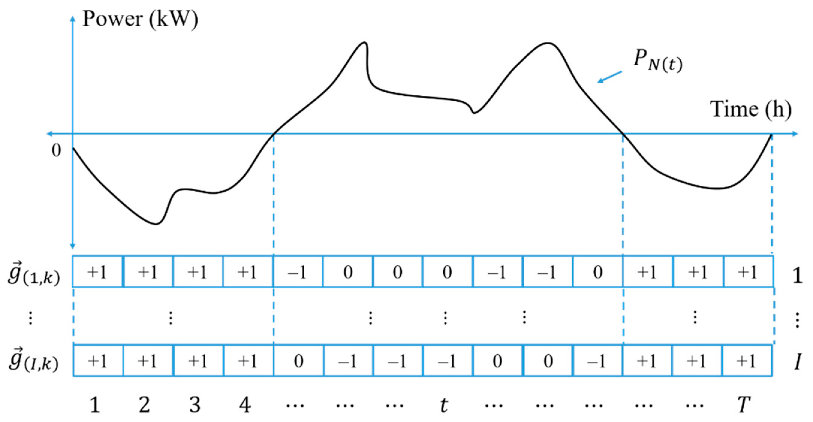
3. Optimization of Day-Ahead Operation

In this section, the optimization problem and the proposed methodology are carefully described. Section 3.1 pays special attention to the objective function definition, whereas Section 3.2 explains how TVMS transfer function is embedded into BPSO for the daily scheduling of BESS.

3.1. Problem Formulation

The focus of this work is on developing a methodology for load peak-shaving to be applied to the management of autonomous HES. In this regard, EMS monitors the state variables of all the elements connected to the point of common coupling (Figure 1). Then, using this information and the day-ahead forecasts of wind power and load demand, determines how power sources should be dispatched to minimize the operating costs of the system for the corresponding day. Note that the influence of forecasting error on system operation has not been considered in this work.

In a general sense, BESS operation can be defined by means of three different states: charging, discharging, and disconnection. These states can be represented by using integers: charging can be represented as +1, discharging can be represented as −1, whereas 0 represents the battery disconnection.

The goal of the management strategy proposed in this paper consists of finding out the appropriate pattern (charging, discharging, and disconnection) of usage of BESS during the day in order to reduce NL-peak. This is carried out by means of a heuristic optimization algorithm in which each individual or agent is represented as shown in Figure 2. If NL is negative, it means that BESS should be charged in order to store the energy surplus during periods of high wind speed. On the contrary, when NL is positive, it is not evident whether BESS should be discharged or disconnected from HES. Thus, a set of $I$ individuals, who take into account different operational conditions (discharging and disconnection) during different hours, is considered.

The structure of a single individual ($i=1,\dots ,I$) at a determined iteration ($k$) of the heuristic optimization algorithm can be described according to (28):

$${\overrightarrow{g}}_{\left(i,k\right)}=\left[\begin{array}{ccc}{g}_{\left(i,1,k\right)}& \begin{array}{ccc}\dots & g_{\left(i,t,k\right)}& \dots \end{array}& g_{\left(i,T,k\right)}\end{array}\right] \forall i=1,\dots ,I;$$

(28)

where each element $g_{\left(i,t,k\right)}$ is an integer between −1 and +1, depending on the time ($t$) and NL value ($P_{N\left(t\right)}$). Similarly, the population or group of agents of the optimization algorithm for iteration $k$ can be expressed as a matrix according to (29):

$$G_{\left(k\right)}=\left[\begin{array}{c}{\overrightarrow{g}}_{\left(1,k\right)}\\ \begin{array}{c}⋮\\ {\overrightarrow{g}}_{\left(i,k\right)}\\ ⋮\end{array}\\ {\overrightarrow{g}}_{\left(I,k\right)}\end{array}\right].$$

(29)

Considering a determined individual $i$, the value of its objective function ($O_{\left(i,k\right)}$) during a determined iteration ($k$), which has to be minimized, is calculated according to (30):

$$O_{\left(i,k\right)}={\displaystyle \sum }_{t=1}^T{P}_{N\left(t\right)}{P}_{C\left(i,t,k\right)} \forall i=1,\dots ,I;k=1,\dots ,K;$$

(30)

where the pattern $P_{C\left(i,t,k\right)}$ corresponds to that obtained from the application of the model previously described in Section 2 (Equation (20)), considering the influence of power converter ($P_{C\left(i,t,k\right)}=P_{C\left(t\right)}$). In other words, $P_{C\left(i,t,k\right)}$ is calculated according to (20), the indexes $i$ and $k$ have been introduced to represent the fact that it is calculated for a specific individual ($i$) during a determined iteration ($k$).

The magnitude presented in (30) does not have any physical meaning. Indeed, this has been taken from previous experience of BESS operating in RTP programs [39], where sold and purchased power all over the day is considered as the optimization variable. Following this analogy, $P_{C\left(i,t,k\right)}$ can be considered as the transaction power of BESS (sold and purchased power), whereas $P_{N\left(t\right)}$ could be considered as linearly related to the fuel-consumption curve of the diesel generator. In other words, in the analogy with selling and purchasing prices under RTP, the variable $P_{N\left(t\right)}$ could be considered as a linear function of fuel-consumption costs.

The main conclusion of this reasoning is that, the hour at which BESS should be discharged, in order to maximize profits from energy trading with the RTP scheme, is exactly the same hour at which BESS should be discharged in order to reduce NL-peak in an autonomous HES.

3.2. Optimization by TVMS-BPSO

PSO is an optimization algorithm based on the dynamic behavior of a group of agents interacting with each other. Important variables such as the position ($g_{\left(i,t,k\right)}$) and velocity ($v_{\left(i,t,k\right)}$) of each agent ($i$) are considered during the evolution of the algorithm ($k$). Using constriction factor approach, the agent velocity can be expressed using (31):

$$v_{\left(i,t,k+1\right)}=\chi \left[v_{\left(i,t,k\right)}+C_{PSO}^a{R}_{PSO}^a\left(g_{\left(t\right)}^{PBEST}-g_{\left(i,t,k\right)}\right)+C_{PSO}^b{R}_{PSO}^b\left(g_{\left(t\right)}^{GBEST}-g_{\left(i,t,k\right)}\right)\right]$$

(31)

where $C_{PSO}^a$ and $C_{PSO}^b$ are coefficients selected so that the condition (32) is fulfilled,

$$\varnothing =C_{PSO}^a+C_{PSO}^b; \varnothing >4.$$

(32)

The coefficient $\varnothing$ is then used to calculate the factor $\chi$ required in (31),

$$\chi =\frac{2}{\left|2-\varnothing -\sqrt{{\varnothing }^2-4\varnothing }\right|}.$$

(33)

Using the coefficient ∅, the convergence of the algorithm can be managed.

TVMS transfer function has been recently proposed by Beheshti [40] to improve the capabilities of BPSO. TVMS-BPSO uses two sigmoid functions during the conversion of reals to binaries, and these functions are shown in (34) and (35):

$$S_{PSO\left(i,t,k+1\right)}^a=\frac{1}{1+e^{{\sigma }_{\left(k\right)}\left(-v_{\left(i,t,k+1\right)}\right)}};$$

(34)

$$S_{PSO\left(i,t,k+1\right)}^b=\frac{1}{1+e^{{\sigma }_{\left(k\right)}\left(v_{\left(i,t,k+1\right)}\right)}};$$

(35)

where the coefficient ${\sigma }_{\left(k\right)}$ varies during the algorithm evolution according to (36):

$${\sigma }_{\left(k\right)}=\left({\sigma }_{max}-{\sigma }_{min}\right)\left(\frac{k}{K}\right)+{\sigma }_{min}.$$

(36)

Once the variables $S_{PSO\left(i,t,k+1\right)}^a$ and $S_{PSO\left(i,t,k+1\right)}^b$ have been calculated, they are evaluated on (37) and (38) to get the binary variables $J_{PSO\left(i,t,k+1\right)}^a$ and $J_{PSO\left(i,t,k+1\right)}^b$, which are a preliminary result of the algorithm.

$$J_{PSO\left(i,t,k+1\right)}^a=\{\begin{array}{c}1; R_{PSO}^c<S_{PSO\left(i,t,k+1\right)}^a\\ 0; R_{PSO}^c\ge S_{PSO\left(i,t,k+1\right)}^a\end{array};$$

(37)

$$J_{PSO\left(i,t,k+1\right)}^b=\{\begin{array}{c}1; R_{PSO}^d<S_{PSO\left(i,t,k+1\right)}^b\\ 0; R_{PSO}^d\ge S_{PSO\left(i,t,k+1\right)}^b\end{array}.$$

(38)

The definitive result from the conversion of reals to binaries is based on the value of the objective function $O_{\left(i,k\right)}^a$ and $O_{i,k}^b$ obtained from the evaluation of $J_{PSO\left(i,t,k+1\right)}^a$ and $J_{PSO\left(i,t,k+1\right)}^b$ previously estimated. Then, the positions to be considered during the next iteration ($k$ + 1) are defined by using (39):

$$g_{\left(i,t,k+1\right)}=\{\begin{array}{c}{J}_{PSO\left(i,t,k+1\right)}^a; O_{PSO\left(i,k+1\right)}^a<O_{PSO\left(i,k+1\right)}^b\\ J_{PSO\left(i,t,k+1\right)}^b; O_{PSO\left(i,k+1\right)}^a>O_{PSO\left(i,k+1\right)}^b\end{array}.$$

(39)

Once the principles of TVMS-BPSO have been exposed. The problem of day-ahead BESS scheduling on a daily basis and the TVMS-BPSO performance to solve this problem are analyzed in Section 4 and Section 5, respectively.

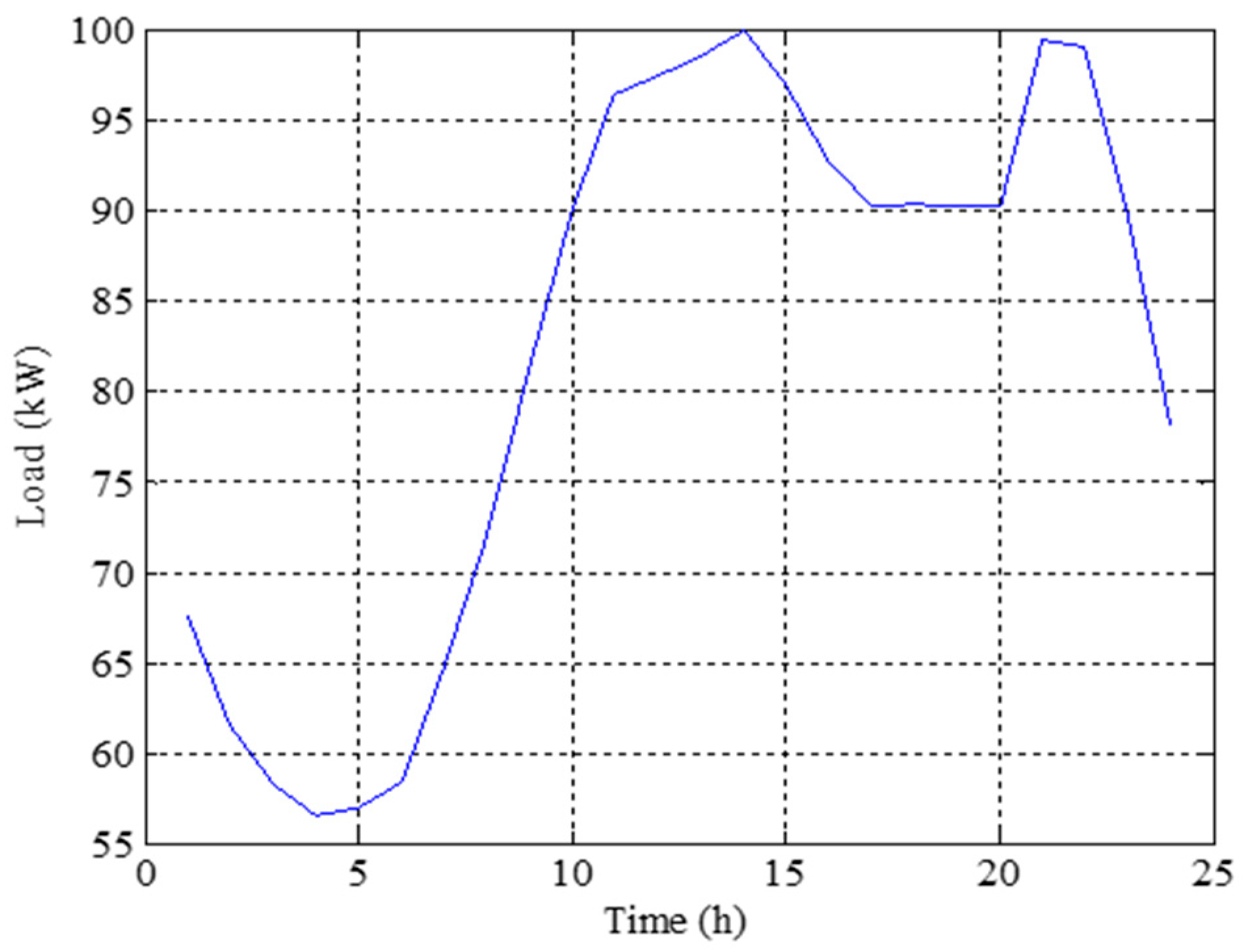
4. Testing the Problem Formulation

To evaluate the mathematical formulation previously presented in Section 3.1, the performance of HES of Figure 1 is analyzed using a GA and a typical system with a wind generator of 75 kW ($P_W^{max}$ = 75 kW), and the load profile of Figure 3 has been used. Cut-in, rated, and cut-out wind speeds equal to 3, 12, and 25 m/s, respectively, have been assumed.

Regarding the fuel-based generator, a diesel unit of 100 kW ($P_D^{max}$ = 100 kW) with minimum operating power of 50% ($P_D^{min}$ = 50 kW) has been assumed.

As the effects of wind generation and BESS management on the reduction of fuel consumption have been deeply studied in the technical literature [41], special attention to the influence of these devices on GHG emissions has been paid in this work. Thus, the GHG-emission measurements published in [42] have been adopted.

During the GA implementation, the initial population is randomly initialized, so that an operator has to be incorporated in order to fix the elements of the matrix $G_{\left(k\right)}$ to +1 at those hours at which NL is negative (Figure 2). Additionally, such operator has to be included after the application of mutation operator.

Regarding the GA parameters, a population with 75 individuals, 100 generations, a crossover rate of 90%, and a mutation rate of 5% were considered.

Wind speed profile has been modeled by using the general purposes profile of (40) [7,10], which depends on the average wind speed ($S_W^a$), diurnal pattern strength ($S_W^b$), and the hour of peak wind speed ($S_W^c$).

$$S_{W\left(t\right)}=S_W^a\left\{1+S_W^{b}cos\left[\left(\frac{2\pi }{T}\right)\left(t-S_W^c\right)\right]\right\} \forall t=1,\dots ,T.$$

(40)

Different values of average wind speed and diurnal pattern strength have been considered. Specifically, $S_W^b$ = 0, 0.1, 0.2, 0.3, 0.4 and $S_W^c$ = 15 h were evaluated through the analysis of three case studies. These are typical values for places located in the United States. In this way, different values of $S_W^b$ allow us to evaluate the wind speed profile with high or low oscillation, and consequently their impact on the operation of BESS.

A typical VRFB of 5 kW/20 kWh ($P_B^{max}$ = 5 kW/ $E_B^{max}$ = 20 kWh) has been considered. Minimum and maximum SOC were assumed as 15 and 90% ($SO{C}_B^{min}$ = 0.15 and $SO{C}_B^{max}$ = 0.9), respectively, and minimum and maximum voltage were assumed as 42 and 56.5 V ($U_B^{min}$ = 42 V and $U_B^{max}$ = 56.5 V), respectively. The entire bank is composed of 10 of these batteries connected in parallel.

The simulation and optimization analysis were implemented in MATLAB^®, using a personal computer with i7-3630QM CPU at 2.4 GHz, 8 GB of memory and a 64-bit operating system.

The previously mentioned cases are carefully discussed in the next subsections.

4.1. Case I: Low Wind Speed with Fully Charged Battery

Conditions of low wind speed and fully charged BESS were simulated by considering an average speed of 4 m/s ($S_W^a$ = 4 m/s) and an initial SOC equal to 85% ($SO{C}_{B\left(0\right)}$ = 0.85).

Figure 4 presents the wind speed (left) and wind power (right) obtained from the evaluation of (40) for the aforementioned values of $S_W^b$. Because the average speed is close to the cut-in one, high wind speed oscillations ($S_W^b$ = 0.4) are directly reflected in the wind power profile.

Figure 5 shows the GA-convergence, which takes around 20 iterations to establish a near-optimal schedule.

Figure 6 presents the day-ahead schedule of BESS for this case. As can be observed, BESS remains disconnected during the morning, between $t$ = 1 h and $t$ = 10 h in all cases. Then, BESS is discharged between $t$ = 11 h and $t$ = 15 h for most of the cases, followed by some disconnection periods, so as to be later discharged during the last hours of the day, between $t$ = 20 h and $t$ = 24 h. These resting intervals or periods of battery disconnection allow us to improve the management of the stored energy by moving it towards the NL-peak hours.

Figure 7 shows the power (left) and SOC (right) of VRFB, where it is possible to observe how battery power is gradually reduced in order to fulfill the operating conditions (16) and (17) for battery voltage and SOC, respectively.

Figure 8 presents NL considering the entire architecture of Figure 1 (left) and only considering the wind and diesel generators (right), calculated using (22) and (21), respectively. According to these results, the proposed peak-shaving strategy is effective at discharging the energy initially stored on BESS during those hours of high electricity demand.

Figure 9 presents THC (left) and CO (right) emissions. By comparing NL considering the effect of wind and BESS previously shown in Figure 8 (left) with THC emissions shown in Figure 9 (left), it is possible to observe how NL has a convex shape, whereas THC emissions have concave behavior, which clearly suggests that THC emissions could increase as NL is reduced. Regarding the relationship between NL (Figure 8 left) and CO emissions (Figure 9 right), concave behavior of both surfaces is clearly observed, which means that CO emissions can be reduced with the corresponding limitation of the NL to be supplied by diesel generator.

Figure 10 shows NO_x (left) and CO₂ (right) emissions, and Figure 11 presents PM emissions. It is possible to observe how all of them slightly increase at the end of the day, due to the fact that BESS management strongly focuses on NL-peak mitigation.

Figure 12 verifies that there is no energy surplus (left) or energy not supplied (right) because renewable generation is very low and the diesel generator is able to supply all electricity demand.

Table 1. Total GHG emissions without battery (Case I).

${\mathit{S}}_{\mathit{W}}^{\mathit{b}}$	THC (kg)	CO (kg)	NOX (kg)	CO2 (kg)	PM (kg)
0	1.37	7.18	31.18	1444.12	0.49
0.1	1.38	7.08	31.13	1442.31	0.48
0.2	1.38	6.94	30.98	1438.01	0.48
0.3	1.39	6.75	30.76	1431.30	0.47
0.4	1.40	6.53	30.47	1422.96	0.46

,

Table 2. Total GHG emissions with battery (Case I).

${\mathit{S}}_{\mathit{W}}^{\mathit{b}}$	THC (g)	CO (g)	NOX (kg)	CO2 (kg)	PM (g)
0	1.57	3.51	24.70	1261.25	0.32
0.1	1.57	3.50	24.65	1260.11	0.32
0.2	1.58	3.36	24.57	1257.46	0.32
0.3	1.58	3.30	24.36	1251.68	0.31
0.4	1.58	3.22	24.09	1244.37	0.31

,

Table 3. Reduction of GHG emissions (Case I).

${\mathit{S}}_{\mathit{W}}^{\mathit{b}}$	THC (%)	CO (%)	NOX (%)	CO2 (%)	PM (%)
0	−14.43	51.19	20.79	12.66	33.54
0.1	−14.10	50.61	20.79	12.63	32.98
0.2	−13.97	51.54	20.68	12.56	33.37
0.3	−13.48	51.09	20.80	12.55	32.72
0.4	−12.92	50.66	20.95	12.55	32.00

and

Table 4. Diesel power generation (Case I).

$\mathit{t}$/${\mathit{S}}_{\mathit{W}}^{\mathit{b}}$	Without BESS					With BESS
	0	0.1	0.2	0.3	0.4	0	0.1	0.2	0.3	0.4
1	66.8	67.3	67.5	67.6	67.6	66.8	67.3	67.5	67.6	67.6
2	60.8	61.3	61.5	61.5	61.5	60.8	61.3	61.5	61.5	61.5
3	57.4	57.9	58.2	58.2	58.2	57.4	57.9	58.2	58.2	58.2
4	55.7	56.2	56.5	56.5	56.5	55.7	56.2	56.5	56.5	56.5
5	56.2	56.6	56.9	56.9	56.9	56.2	56.6	56.9	56.9	56.9
6	57.6	58.0	58.3	58.4	58.4	57.6	58.0	58.3	58.4	58.4
7	63.9	64.2	64.4	64.6	64.6	63.9	64.2	64.4	64.6	64.6
8	71.0	71.2	71.3	71.4	71.5	71.0	71.2	71.3	71.4	71.5
9	80.6	80.6	80.6	80.6	80.6	80.6	80.6	80.6	80.6	80.6
10	89.2	89.0	88.8	88.6	88.3	89.2	89.0	88.8	88.6	88.3
11	95.7	95.3	94.9	94.3	93.7	58.4	58.0	57.6	57.0	56.4
12	96.7	96.2	95.5	94.6	93.6	61.6	61.0	60.3	59.5	58.4
13	97.8	97.1	96.2	95.0	93.6	64.7	64.0	63.0	61.9	60.5
14	99.2	98.4	97.4	96.0	94.4	68.1	67.3	66.2	64.9	63.2
15	96.1	95.3	94.1	92.7	91.0	66.9	66.0	64.9	63.4	61.7
16	91.9	91.1	90.0	88.7	87.0	64.4	63.6	62.6	61.2	87.0
17	89.4	88.7	87.8	86.6	85.2	89.4	88.7	87.8	86.6	85.2
18	89.6	89.1	88.4	87.5	86.5	63.8	63.2	88.4	87.5	86.5
19	89.4	89.0	88.6	88.1	87.4	67.4	67.0	88.6	88.1	60.0
20	89.4	89.2	89.0	88.8	88.5	79.5	79.3	63.2	62.9	62.7
21	98.6	98.6	98.6	98.6	98.6	94.3	94.3	76.6	76.6	76.6
22	98.2	98.4	98.5	98.6	98.7	95.9	96.0	88.6	88.8	88.9
23	88.8	89.1	89.3	89.5	89.5	87.2	87.6	85.0	85.2	85.2
24	77.3	77.7	77.9	78.0	78.0	76.1	76.6	75.6	75.7	75.7

summarize the daily results related to GHG emissions and diesel generation. By comparing the second columns of Table 1 and Table 2, it is possible to observe how THC emissions increase as previously discussed. In the contrary case, a reduction on CO, NO_x, CO₂, and PM is clearly observed.

Table 3 shows the change on GHG emissions based on the results reported in Table 1 and Table 2. The increment of THC emissions is between 12.92% and 14.43%, whereas the reduction of CO, NO_x, CO₂, and PM are approximately 51.02%, 20.80%, 12.59%, and 32.92%, respectively.

Table 4 shows in bold those hours at which power generation is reduced as a result of BESS incorporation, especially during the peak-load of the afternoon and night.

4.2. Case II: High Wind Speed with Empty Battery

In this case, conditions of high wind speed with an empty battery are studied. Specifically, an average wind speed of 14 m/s ($S_W^a$ = 14 m/s) and an initial SOC of 15% ($SO{C}_{B\left(0\right)}$ = 0.15) are considered. Wind speed and wind power under these conditions are shown in Figure 13, in the left and right sides, respectively, for $S_W^b$ between 0 and 0.4, as previously specified.

According to the wind power profile (Figure 13 right), rating power is reached in almost all cases, except when a high wind speed oscillation ($S_W^b\to$0.4) is observed, resulting in a wind power reduction during the morning.

GA evolution is shown in Figure 14, where it can be observed how fast the algorithm converges due to the influence of the high wind speed. In other words, in the presence of high wind speed, the energy surplus forces BESS to be charged, limiting the number of possible operational combinations, and consequently speeding up the convergence.

BESS management is shown in Figure 15, where the battery is charged during the morning in most situations. However, discharging actions are also advised sometimes in the morning, and this is observed when wind generation reduces as a consequence of wind speed profile oscillations. Initially, the battery is empty, so that discharging the battery in this situation does not result in any load satisfaction, because the battery is not able to provide any power. In other words, battery discharge when $SO{C}_{B\left(t\right)}=SO{C}_B^{min}$ is equivalent to the battery disconnection obtained by setting $g_{\left(i,t,k\right)}\leftarrow$0.

Figure 16 shows the results obtained from the simulation of the management signal previously shown in Figure 15. Battery power (Figure 16 left) and SOC (Figure 16 right) are presented, and the battery is charged during the morning and then discharged during the afternoon. The situations of high wind speed oscillations result in a reduction of energy surplus, and consequently less power is available to be used in the peak-shaving process during the afternoon.

Figure 17 shows the NL profile depending on if the effects of BESS are considered (left) or not (right), calculated by using (22) and (21), respectively. By comparing these results, it is possible to observe how NL-peak is reduced.

As NL is so low when BESS is incorporated, energy surplus is produced because the diesel generator is forced to operate at its minimum capacity in order to satisfy a very low load. This operating mode produces a fixed amount of GHG emissions. This reasoning can be verified in Figure 18 for THC (left) and CO (right), in Figure 19 for NO_X (left) and CO₂ (right), and in Figure 20 for PM.

Figure 21 shows the daily profiles of energy surplus (left) and ENS (right), respectively. As wind generation is abundant from the high wind speed, energy excess is observed at almost any time. Conversely, there is no ENS.

Table 5. Total GHG emissions without battery (Case II).

${\mathit{S}}_{\mathit{W}}^{\mathit{b}}$	THC (kg)	CO (kg)	NOX (kg)	CO2 (kg)	PM (kg)
0	1.17	0.62	8.48	629.60	0.14
0.1	1.17	0.62	8.48	629.60	0.14
0.2	1.17	0.62	8.48	629.60	0.14
0.3	1.53	0.82	11.13	826.35	0.19
0.4	1.68	0.90	12.19	905.05	0.21

and

Table 6. Total GHG emissions with battery (Case II).

${\mathit{S}}_{\mathit{W}}^{\mathit{b}}$	THC (kg)	CO (kg)	NOX (kg)	CO2 (kg)	PM (kg)
0	1.02	0.55	7.42	550.90	0.13
0.1	1.02	0.55	7.42	550.90	0.13
0.2	1.10	0.59	7.95	590.25	0.14
0.3	1.53	0.82	11.13	826.35	0.19
0.4	1.68	0.90	12.19	905.05	0.21

report the cumulative daily values of GHG emissions for different wind speed profiles. Then, the reduction on the emitted pollutants as a consequence of BESS integration is reported in

Table 7. Reduction of GHG emissions (Case II).

${\mathit{S}}_{\mathit{W}}^{\mathit{b}}$	THC (%)	CO (%)	NOX (%)	CO2 (%)	PM (%)
0	12.5	12.5	12.5	12.5	12.5
0.1	12.5	12.5	12.5	12.5	12.5
0.2	6.25	6.25	6.25	6.25	6.25
0.3	0	0	0	0	0
0.4	0	0	0	0	0

. Because the diesel generator is operating at its minimum allowed power ($P_{D\left(t\right)}=P_D^{min}$), the reduction of GHG emissions is the same for all the factors considered, up to 12.5%.

To improve understanding of the HES operation,

Table 8. Diesel power generation (Case II).

$\mathit{t}$/${\mathit{S}}_{\mathit{W}}^{\mathit{b}}$	Without BESS					With BESS
	0	0.1	0.2	0.3	0.4	0	0.1	0.2	0.3	0.4
1	0	0	0	50	50	0	0	0	50	50
2	0	0	0	50	50	0	0	0	50	50
3	0	0	0	50	50	0	0	0	50	50
4	0	0	0	50	50	0	0	0	50	50
5	0	0	0	50	50	0	0	0	50	50
6	0	0	0	0	50	0	0	0	0	50
7	0	0	0	0	50	0	0	0	0	50
8	0	0	0	0	0	0	0	0	0	0
9	50	50	50	50	50	50	50	50	50	50
10	50	50	50	50	50	50	50	50	50	50
11	50	50	50	50	50	50	50	50	50	50
12	50	50	50	50	50	0	0	50	50	50
13	50	50	50	50	50	0	0	0	50	50
14	50	50	50	50	50	50	50	50	50	50
15	50	50	50	50	50	50	50	50	50	50
16	50	50	50	50	50	50	50	50	50	50
17	50	50	50	50	50	50	50	50	50	50
18	50	50	50	50	50	50	50	50	50	50
19	50	50	50	50	50	50	50	50	50	50
20	50	50	50	50	50	50	50	50	50	50
21	50	50	50	50	50	50	50	50	50	50
22	50	50	50	50	50	50	50	50	50	50
23	50	50	50	50	50	50	50	50	50	50
24	50	50	50	50	50	50	50	50	50	50

presents the output power of the diesel generator with and without considering the BESS operation. In bold are shown those situations where the diesel unit is disconnected, all of them during the first peak between $t$ = 12 h and $t$ = 13 h.

4.3. Case III: Very High Wind Speed with Empty Battery

In this case, conditions of extreme wind speed are analyzed by setting the average speed to 24 m/s ($S_W^a$ = 24 m/s), while the battery remains empty ($SO{C}_{B\left(0\right)}$ = 0.15).

Figure 22 shows the wind speed (left) and wind power (right) for this case. As wind speed becomes higher than the cut-out speed (25 m/s) for those cases with wind speed oscillation, the wind turbine is taken out of service in order to preserve it. Thus, NL suddenly increases during the afternoon.

GA evolution is shown in Figure 23, where a fast convergence is observed due to the fact that the battery has to be charged during the first hours of the day, reducing the number of possible combinations of the optimization problem.

Management signal is shown in Figure 24. According to these results, battery should be charged during the morning. Then, a short resting period is advised so that enough energy is available to be discharged during the peak-load hours.

Charging and discharging cycles are represented by means of the battery power and SOC shown in Figure 25 at the left and right sides, respectively.

The reduction of NL as a result of BESS integration can be observed at the left side of Figure 26. NL without considering the influence of BESS is presented at the right side of Figure 26, where the increment of load demand during the afternoon can be clearly observed.

GHG emissions are fully described in Figure 27, Figure 28 and Figure 29, where the lack of wind generation during the afternoon, as a result of the extremely high wind speed, directly influences the behavior of all emission factors.

Energy surplus and ENS are reported in the left and right sides of Figure 30, respectively, where the energy excess is directly related to the operation of the diesel generator during the afternoon. As expected, there is no ENS because the diesel generator is able to supply any value of electricity demand.

Table 9. Total GHG emissions without battery (Case III).

${\mathit{S}}_{\mathit{W}}^{\mathit{b}}$	THC (kg)	CO (kg)	NOX (kg)	CO2 (kg)	PM (kg)
0	1.17	0.62	8.48	629.60	0.14
0.1	0.94	4.59	18.35	899.93	0.32
0.2	0.90	5.28	20.30	953.02	0.35
0.3	0.90	5.28	20.30	953.02	0.35
0.4	0.90	5.28	20.30	953.02	0.35

,

Table 10. Total GHG emissions with battery (Case III).

${\mathit{S}}_{\mathit{W}}^{\mathit{b}}$	THC (kg)	CO (kg)	NOX (kg)	CO2 (kg)	PM (kg)
0	1.02	0.55	7.42	550.90	0.13
0.1	1.02	2.89	16.05	833.17	0.24
0.2	0.98	3.59	18.01	886.27	0.27
0.3	0.98	3.59	18.01	886.27	0.27
0.4	0.98	3.59	18.01	886.27	0.27

,

Table 11. Reduction of GHG emissions (Case III).

${\mathit{S}}_{\mathit{W}}^{\mathit{b}}$	THC (%)	CO (%)	NOX (%)	CO2 (%)	PM (%)
0	12.50	12.50	12.50	12.50	12.50
0.1	−9.30	36.98	12.51	7.42	23.93
0.2	−9.73	32.12	11.31	7.00	21.86
0.3	−9.73	32.12	11.31	7.00	21.86
0.4	−9.73	32.12	11.31	7.00	21.86

and

Table 12. Diesel power generation (Case III).

$\mathit{t}$/${\mathit{S}}_{\mathit{W}}^{\mathit{b}}$	Without BESS					With BESS
	0	0.1	0.2	0.3	0.4	0	0.1	0.2	0.3	0.4
1	0	0	0	0	0	0	0	0	0	0
2	0	0	0	0	0	0	0	0	0	0
3	0	0	0	0	0	0	0	0	0	0
4	0	0	0	0	0	0	0	0	0	0
5	0	0	0	0	0	0	0	0	0	0
6	0	0	0	0	0	0	0	0	0	0
7	0	0	0	0	0	0	0	0	0	0
8	0	0	0	0	0	0	0	0	0	0
9	50	50	50	50	50	50	50	50	50	50
10	50	50	90	90	90	50	50	90	90	90
11	50	96.4	96.4	96.4	96.4	50	96.4	96.4	96.4	96.4
12	50	97.5	97.5	97.5	97.5	0	70.2	70.2	70.2	70.2
13	50	98.5	98.5	98.5	98.5	0	72.9	72.9	72.9	72.9
14	50	100	100	100	100	50	79.7	79.7	79.7	79.7
15	50	96.9	96.9	96.9	96.9	50	87.9	87.9	87.9	87.9
16	50	92.7	92.7	92.7	92.7	50	88.7	88.7	88.7	88.7
17	50	90.2	90.2	90.2	90.2	50	88	90.2	90.2	90.2
18	50	90.4	90.4	90.4	90.4	50	88.9	88.2	88.2	88.2
19	50	90.2	90.2	90.2	90.2	50	89.1	88.7	88.7	88.7
20	50	50	90.2	90.2	90.2	50	50	89.1	89.1	89.1
21	50	50	50	50	50	50	50	50	50	50
22	50	50	50	50	50	50	50	50	50	50
23	50	50	50	50	50	50	50	50	50	50
24	50	50	50	50	50	50	50	50	50	50

summarize the GHG emissions and diesel generation for this case. By comparing Table 9 and Table 10, it is possible to observe that, in some situations, THC emissions can increase when BESS reduces NL in a considerable manner. Regarding the wind speed oscillation, as $S_W^b$ increases, wind speed in the hours close to 15 h ($S_W^c$ = 15 h) increases to a value higher than cut-out speed (25 m/s), removing the wind power generation. Thus, BESS supplies a part of the required power, but essentially most of it is provided by the diesel generator, increasing even more the emissions of CO, NO_x, CO₂, and PM to the atmosphere.

In Table 12, it can be observed how the diesel generator reduces its power production or is disconnected. This happens in those hours between $t$ = 12 h and $t$ = 20 h, when BESS has an active role in mitigating NL.

From the sensitivity analysis of Cases I-III, it is possible to conclude that the objective function defined in (30) offers reasonable results in terms of BESS management for peak-shaving. The next section studies the performance of TVMS-BPSO implemented to minimize this already tested objective function.

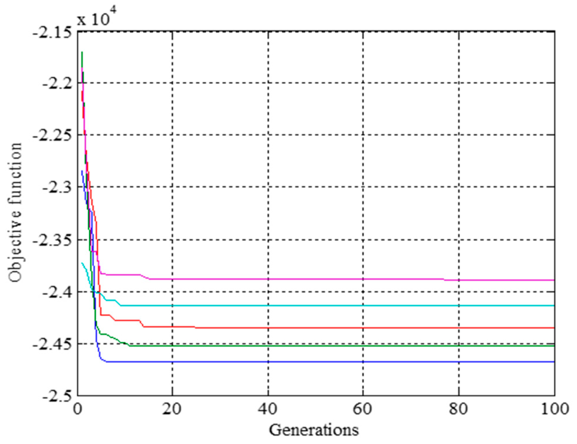
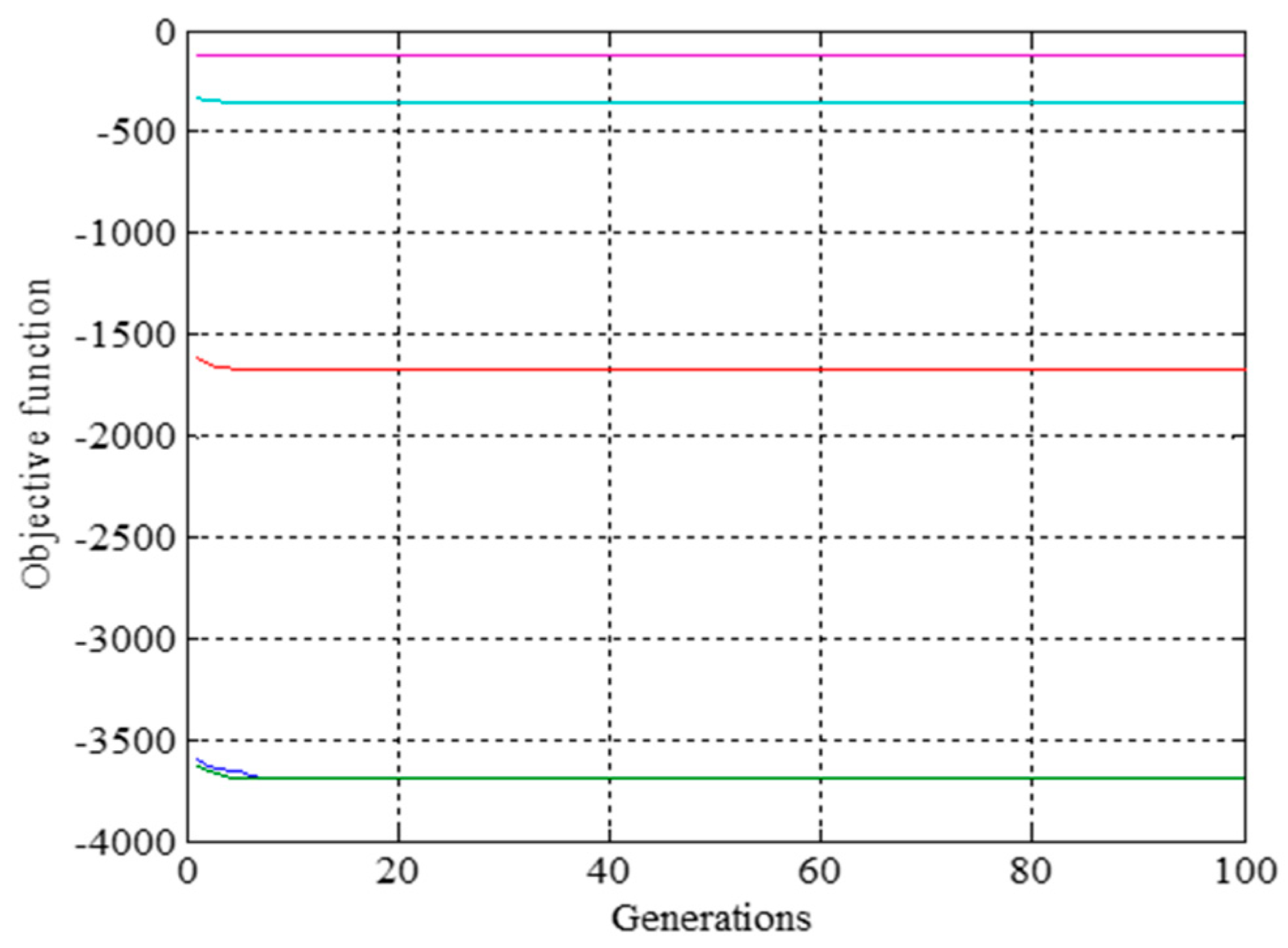
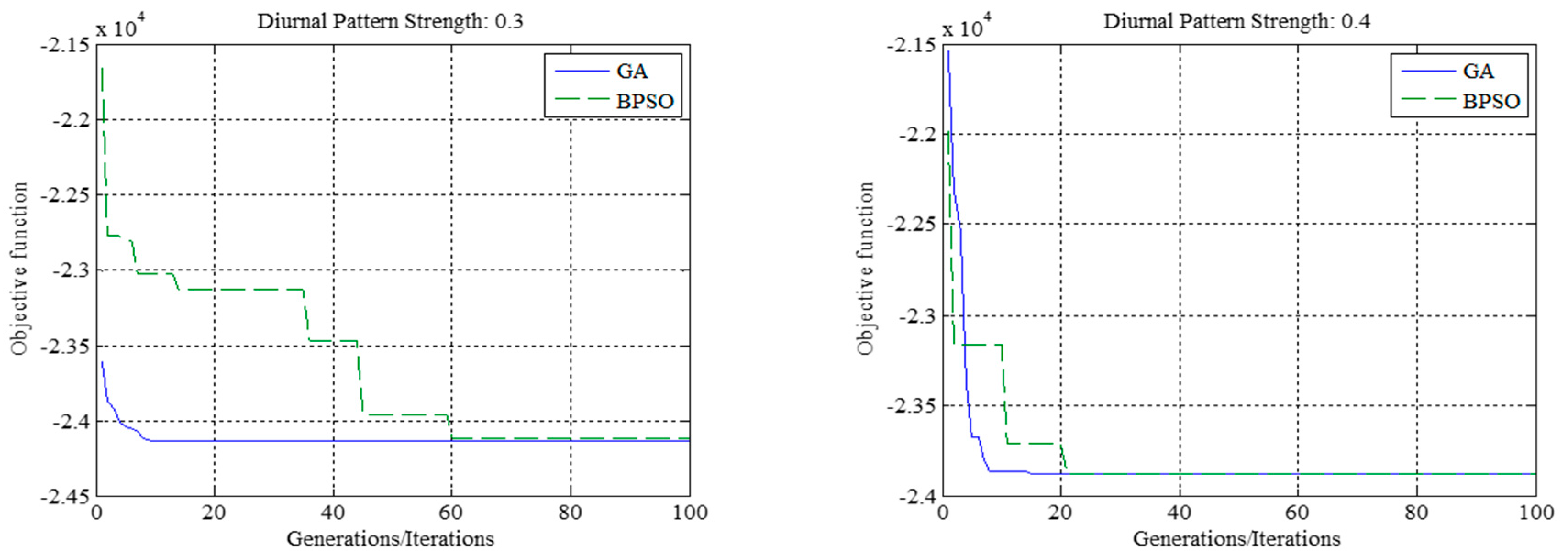
5. Performance of TVMS-BPSO

To evaluate the capabilities of TVMS-BPSO presented in Section 3.2 for day-ahead BESS scheduling, the conditions of Case I (low wind speed with fully charged battery) previously described in Section 4.1 have been considered. This case has been chosen because the number of optimization variables to be determined is the highest. Regarding the number of agents and iterations, these have been set equal to the population size and generations of GA previously implemented in Section 4 (75 agents and 100 iterations), and this guarantees a fair comparison between both methods. Other parameters of BPSO have been adjusted as follows; $C_{PSO}^a$ = 2.05, $C_{PSO}^b$ = 2.05, ${\sigma }_{min}$ = 0.1, and ${\sigma }_{max}$ = 1.

Figure 31, Figure 32 and Figure 33 show the comparison between GA and TVMS-BPSO for different wind speed profiles, whereas

Table 13. Comparison of objective function values.

${\mathit{S}}_{\mathit{W}}^{\mathit{b}}$	GA	BPSO	Difference (%)
0	−24,680.21	−24,679.41	0.00326
0.1	−24,528.93	−24,520.42	0.03469
0.2	−24,348.18	−24,331.04	0.07039
0.3	−24,134.06	−24,116.79	0.07154
0.4	−23,877.54	−23,877.54	0

shows the value of the objective function. As can be observed, TVMS-BPSO employs global exploration during the first iterations, analyzing solutions with high objective function value. As the algorithm evolves, exploitation has the relevant role of guiding the algorithm to a high quality solution, comparable to that obtained from GA implementation, according to Table 13.

6. Conclusions and Remarks

The results obtained from the analysis of the aforementioned cases offer us important lessons about the mitigation of GHG emissions by integrating a BESS managed from a purely economic perspective. The proposed approach is based on the solution of an optimization problem in which the number of possible combinations varies with the available wind speed profile.

As NL becomes negative, the management signal of BESS is directly set to the charging process ($g_{\left(i,t,k\right)}$ = +1). In the contrary case, when NL is positive, the optimization approach has to determine whether the BESS should be discharged ($g_{\left(i,t,k\right)}$ = −1) or disconnected ($g_{\left(i,t,k\right)}$ = 0) to reduce the daily NL-peak.

Let $T$ be the number of hours during which NL is positive (Case I Section 4.1), the number of decision variables to be determined is defined as $2^T$. In Case I, the wind speed profile was so low that no energy surplus was observed. However, the initial SOC was high, so that the proposed approach had to determine how to use that stored energy in order to reduce NL-peak. Under these circumstances, $T$ = 24 and the number of possible combinations is 16,777,216. That is why GA and TVMS-BPSO require some iterations to get a near-optimal solution (Figure 5, Figure 31, Figure 32 and Figure 33). Conversely, as wind speed increases, as studied in Case II and Case III, energy surplus increases and the number of combinations is reduced, making the management problem easier to solve. This is why an extremely fast convergence is observed in Figure 14 and Figure 23, for Case II and Case III, respectively. With respect to TVMS-BPSO performance, its important capabilities for global exploration and local exploitation offer a high quality solution similar to that obtained from GA implementation (Table 13).

Regarding GHG emissions, the highest reduction was observed in Case I, in which wind power generation was very low, but available energy from BESS was optimally allocated. As Table 3, Table 7, and Table 11 were calculated using the wind–diesel system as reference, Case I presents the highest percentage of reduction. As long as wind speed increases, the diesel generator must be committed to its minimum capacity so that GHG emissions cannot be totally eliminated, and this is important for the optimal sizing of HES. In the presence of an extremely high wind speed, when the wind turbine is disconnected, the reduction of GHG emissions highly depends on how BESS is managed, which can be observed in the results of Case III (Table 11), specifically. Another relevant result is that THC emissions do not always increase with the partial operation of the diesel unit: in Case II, THC emissions were reduced, perhaps because the diesel generator was disconnected in some operational circumstances.

References

1. Rogelj, J.; Huppmann, D.; Krey, V.; Riahi, K.; Clarke, L.; Gidden, M.; Nicholls, Z.; Meinshausen, M. A new scenario logic for the Paris Agreement long-term temperature goal. Nature 2019, 573, 357–363. [Google Scholar] [CrossRef]
2. Pfeifer, A.; Krajačić, G.; Ljubas, D.; Duić, N. Increasing the integration of solar photovoltaics in energy mix on the road to low emissions energy system—Economic and environmental implications. Renew. Energy 2019, 143, 1310–1317. [Google Scholar] [CrossRef]
3. Martí-Ballester, C.-P. Do European renewable energy mutual funds foster the transition to a low-carbon economy? Renew. Energy 2019, 143, 1299–1309. [Google Scholar] [CrossRef]
4. Arbabzadeh, M.; Sioshansi, R.; Johnson, J.X.; Keoleian, G.A. The role of energy storage in deep decarbonization of electricity production. Nat. Commun. 2019, 10, 1–11. [Google Scholar] [CrossRef]
5. Sgouridis, S.; Carbajales-Dale, M.; Csala, D.; Chiesa, M.; Bardi, U. Comparative net energy analysis of renewable electricity and carbon capture and storage. Nat. Energy 2019, 4, 456–465. [Google Scholar] [CrossRef]
6. Comello, S.; Reichelstein, S. The emergence of cost effective battery storage. Nat. Commun. 2019, 10, 1–9. [Google Scholar] [CrossRef]
7. HOMER Pro. Available online: https://www.homerenergy.com/ (accessed on 14 October 2019).
8. iHOGA. Available online: https://ihoga.unizar.es/ (accessed on 14 October 2019).
9. Hybrid2. Available online: https://www.umass.edu/ (accessed on 14 October 2019).
10. Lambert, T.; Gilman, P.; Lilienthal, P. Micropower system modeling with HOMER. In Integration of Alternative Sources of Energy, 1st ed.; Farret, F.A., Simões, M.G., Eds.; Wiley-IEEE Press: Hoboken, NJ, USA, 2006; pp. 379–418. [Google Scholar]
11. Li, Q.; Choi, S.S.; Yuan, Y.; Yao, D.L. On the determination of battery energy storage capacity and short-term power dispatch of a wind farm. IEEE Trans. Sustain. Energy 2011, 2, 148–158. [Google Scholar] [CrossRef]
12. Luo, F.; Meng, K.; Dong, Z.Y.; Zheng, Y.; Chen, Y.; Wong, K.P. Coordinated operational planning for wind farm with battery energy storage system. IEEE Trans. Sustain. Energy 2015, 6, 253–262. [Google Scholar] [CrossRef]
13. Mohammadi, S.; Mozafari, B.; Solymani, S.; Niknam, T. Stochastic scenario-based model and investigating size of energy storages for PEM-fuel cell unit commitment of micro-grid considering profitable strategies. IET Gener. Transm. Distrib. 2014, 8, 1228–1243. [Google Scholar] [CrossRef]
14. O’Dwyer, C.; Flynn, D. Using energy storage to manage high net load variability at sub-hourly time-scales. IEEE Trans. Power Syst. 2015, 30, 2139–2148. [Google Scholar] [CrossRef]
15. Wen, Y.; Guo, C.; Pandžić, H.; Kirschen, D.S. Enhanced security-constrained unit commitment with emerging utility-scale energy storage. IEEE Trans. Power Syst. 2016, 31, 652–662. [Google Scholar] [CrossRef]
16. Wen, Y.; Li, W.; Huang, G.; Liu, X. Frequency dynamics constrained unit commitment with battery energy storage. IEEE Trans. Power Syst. 2016, 31, 5115–5125. [Google Scholar] [CrossRef]
17. Nguyen, T.A.; Crow, M.L. Stochastic optimization of renewable-based microgrid operation incorporating battery operating cost. IEEE Trans. Power Syst. 2016, 31, 2289–2296. [Google Scholar] [CrossRef]
18. Khorramdel, H.; Aghaei, J.; Khorramdel, B.; Siano, P. Optimal battery sizing in microgrids using probabilistic unit commitment. IEEE Trans. Ind. Inform. 2016, 12, 834–843. [Google Scholar] [CrossRef]
19. Li, N.; Uçkun, C.; Constantinescu, E.M.; Birge, J.R.; Hedman, K.W.; Botterud, A. Flexible operation of batteries in power system scheduling with renewable energy. IEEE Trans. Sustain. Energy 2016, 7, 685–696. [Google Scholar] [CrossRef]
20. Jiang, Y.; Xu, J.; Sun, Y.; Wei, C.; Wang, J.; Ke, D.; Li, X.; Yang, J.; Peng, X.; Tang, B. Day-ahead stochastic economic dispatch of wind integrated power system considering demand response of residential hybrid energy system. Appl. Energy 2017, 190, 1126–1137. [Google Scholar] [CrossRef]
21. Anand, H.; Ramasubbu, R. A real time pricing strategy for remote micro-grid with economic emission dispatch and stochastic renewable energy sources. Renew. Energy 2018, 127, 779–789. [Google Scholar] [CrossRef]
22. Wu, X.; Zhang, K.; Cheng, M.; Xin, X. A switched dynamical system approach towards the economic dispatch of renewable hybrid power systems. Int. J. Electr. Power Energy Syst. 2018, 103, 440–457. [Google Scholar] [CrossRef]
23. Dui, X.; Zhu, G.; Yao, L. Two-stage optimization of battery energy storage capacity to decrease wind power curtailment in grid-connected wind farms. IEEE Trans. Power Syst. 2018, 33, 3296–3305. [Google Scholar] [CrossRef]
24. Psarros, G.N.; Karamanou, E.G.; Papathanassiou, S.A. Feasibility analysis of centralized storage facilities in isolated grids. IEEE Trans. Sustain. Energy 2018, 9, 1822–1832. [Google Scholar] [CrossRef]
25. Psarros, G.N.; Papathanassiou, S.A. Internal dispatch for RES-storage hybrid power stations in isolated grids. Renew. Energy 2020, 147, 2141–2150. [Google Scholar] [CrossRef]
26. Ahmadi, A.; Nezhad, A.E.; Hredzak, B. Security-constrained unit commitment in presence of lithium-ion battery storage units using information-gap decision theory. IEEE Trans. Ind. Inform. 2019, 15, 148–157. [Google Scholar] [CrossRef]
27. Saleh, S.A. Testing a unit commitment based controller for grid-connected PMG-based WECSs with generator-charged battery units. IEEE Trans. Ind. Appl. 2019, 55, 2185–2197. [Google Scholar] [CrossRef]
28. Gupta, P.P.; Jain, P.; Sharma, S.; Sharma, K.C.; Bhakar, R. Stochastic scheduling of battery energy storage system for large-scale wind power penetration. J. Eng. 2019, 2019, 5028–5032. [Google Scholar]
29. Alvarez, M.; Rönnberg, S.K.; Bermúdez, J.; Zhong, J.; Bollen, M.H.J. A generic storage model based on a future cost piecewise-linear approximation. IEEE Trans. Smart Grid 2019, 10, 878–888. [Google Scholar] [CrossRef]
30. Chen, L.; Zhu, X.; Cai, J.; Xu, X.; Liu, H. Multi-time scale coordinated optimal dispatch of microgrid cluster based on MAS. Electr. Power Syst. Res. 2019, 177, 105976. [Google Scholar] [CrossRef]
31. Tan, Q.; Ding, Y.; Ye, Q.; Mei, S.; Zhang, Y.; Wei, Y. Optimization and evaluation of a dispatch mode for an integrated wind-photovoltaic-thermal power system based on dynamic carbon emissions trading. Appl. Energy 2019, 253, 113598. [Google Scholar] [CrossRef]
32. Yiwei, F.; Zongxiang, L.; Wei, H.; Shuang, W.; Yiting, W.; Ling, D.; Jietan, Z. Research on joint optimal dispatching method for hybrid power system considering system security. Appl. Energy 2019, 238, 147–163. [Google Scholar]
33. Giorsetto, P.; Utsurogi, K.F. Development of a new procedure for reliability modeling of wind generating units. IEEE Trans. Power Appar. Syst. 1983, PAS-102, 134–143. [Google Scholar] [CrossRef]
34. Dialynas, E.N.; Machias, A.V. Reliability modelling interactive techniques of power systems including wind generating units. Archiv Elektrotechnik 1989, 72, 33–41. [Google Scholar] [CrossRef]
35. Qiu, X.; Nguyen, T.A.; Guggenberger, J.D.; Crow, M.L.; Elmore, A.C. A field validated model of a vanadium redox flow battery for microgrids. IEEE Trans. Smart Grid 2014, 5, 1592–1601. [Google Scholar] [CrossRef]
36. Nguyen, T.A.; Qiu, X.; Guggenberger, J.D., II; Crow, M.L.; Elmore, A.C. Performance characterization for photovoltaic-vanadium redox battery microgrid systems. IEEE Trans. Sustain. Energy 2014, 5, 1379–1388. [Google Scholar] [CrossRef]
37. Nguyen, T.A.; Crow, M.L.; Elmore, A.C. Optimal sizing of a vanadium redox battery system for microgrid systems. IEEE Trans. Sustain. Energy 2015, 6, 729–737. [Google Scholar] [CrossRef]
38. Rampinelli, G.A.; Krenzinger, A.; Romero, F.C. Mathematical models for efficiency of inverters used in grid connected photovoltaic systems. Renew. Sustain. Energy Rev. 2014, 34, 578–587. [Google Scholar] [CrossRef]
39. Lujano-Rojas, J.M.; Dufo-López, R.; Bernal-Agustín, J.L.; Catalão, J.P.S. Optimizing daily operation of battery energy storage systems under real-time pricing schemes. IEEE Trans. Smart Grid 2017, 8, 316–330. [Google Scholar] [CrossRef]
40. Beheshti, Z. A time-varying mirrored S-shaped transfer function for binary particle swarm optimization. Inf. Sci. 2019. [Google Scholar] [CrossRef]
41. Lujano-Rojas, J.M.; Dufo-López, R.; Bernal-Agustín, J.L. Technical and economic effects of charge controller operation and coulombic efficiency on stand-alone hybrid power systems. Energy Convers. Manag. 2014, 86, 709–716. [Google Scholar] [CrossRef]
42. Shah, S.D.; Cocker, D.R., III; Johnson, K.C.; Lee, J.M.; Soriano, B.L.; Miller, J.W. Emissions of regulated pollutants from in-use diesel back-up generators. Atmos. Environ. 2006, 40, 4199–4209. [Google Scholar] [CrossRef]
Figure 1. Hybrid energy system (HES) under study.
Applsci 09 05221 g001
Figure 2. Structure of a single individual.
Applsci 09 05221 g002
Figure 3. Load profile.
Applsci 09 05221 g003
Figure 4. Wind speed and wind power (Case I).
Applsci 09 05221 g004
Figure 5. Genetic algorithm (GA) evolution (Case I).
Applsci 09 05221 g005
Figure 6. Battery management (Case I).
Applsci 09 05221 g006
Figure 7. Battery power and state of charge (SOC) (Case I).
Applsci 09 05221 g007
Figure 8. Net load with and without battery (Case I).
Applsci 09 05221 g008
Figure 9. THC and CO emissions (Case I).
Applsci 09 05221 g009
Figure 10. NOX and CO2 emissions (Case I).
Applsci 09 05221 g010
Figure 11. PM emissions (Case I).
Applsci 09 05221 g011
Figure 12. Excess and energy not supplied (ENS) (Case I).
Applsci 09 05221 g012
Figure 13. Wind speed and wind power (Case II).
Applsci 09 05221 g013
Figure 14. GA evolution (Case II).
Applsci 09 05221 g014
Figure 15. Battery management (Case II).
Applsci 09 05221 g015
Figure 16. Battery power and SOC (Case II).
Applsci 09 05221 g016
Figure 17. Net load with and without battery (Case II).
Applsci 09 05221 g017
Figure 18. THC and CO emissions (Case II).
Applsci 09 05221 g018
Figure 19. NOX and CO2 emissions (Case II).
Applsci 09 05221 g019
Figure 20. PM emissions (Case II).
Applsci 09 05221 g020
Figure 21. Excess and ENS (Case II).
Applsci 09 05221 g021
Figure 22. Wind speed and wind power (Case III).
Applsci 09 05221 g022
Figure 23. GA evolution (Case III).
Applsci 09 05221 g023
Figure 24. Battery management (Case III).
Applsci 09 05221 g024
Figure 25. Battery power and SOC (Case III).
Applsci 09 05221 g025
Figure 26. Net load with and without battery (Case III).
Applsci 09 05221 g026
Figure 27. THC and CO emissions (Case III).
Applsci 09 05221 g027
Figure 28. NOX and CO2 emissions (Case III).
Applsci 09 05221 g028
Figure 29. PM emissions (Case III).
Applsci 09 05221 g029
Figure 30. Excess and ENS (Case III).
Applsci 09 05221 g030
Figure 31. TVMS-BPSO evolution for diurnal pattern strength equal to 0.
Applsci 09 05221 g031
Figure 32. TVMS-BPSO evolution for diurnal pattern strength equal to 0.1 and 0.2.
Applsci 09 05221 g032
Figure 33. X. TVMS-BPSO evolution for diurnal pattern strength equal to 0.3 and 0.4.
Applsci 09 05221 g033