Adaptive Pitch Control of Variable-Pitch PMSG Based Wind Turbine


Abstract
:1. Introduction
2. Model and Problem Formulation
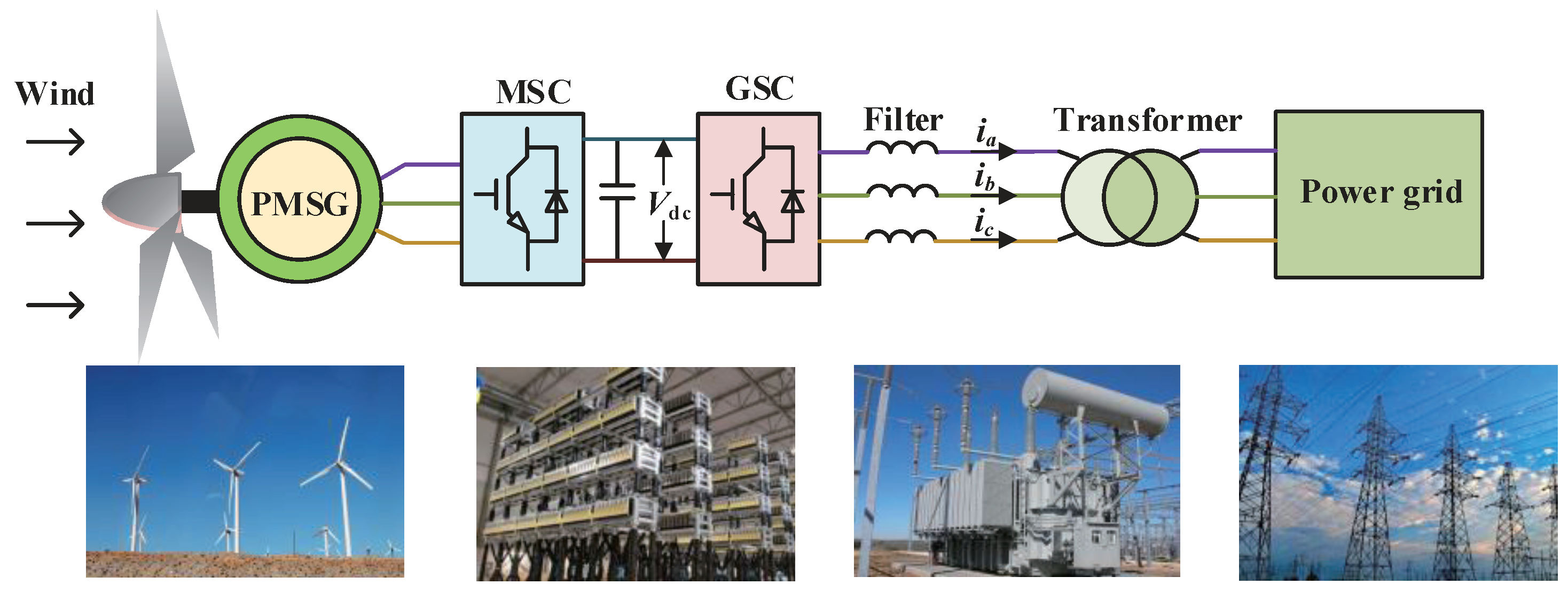
2.1. PMSG-WT Configuration
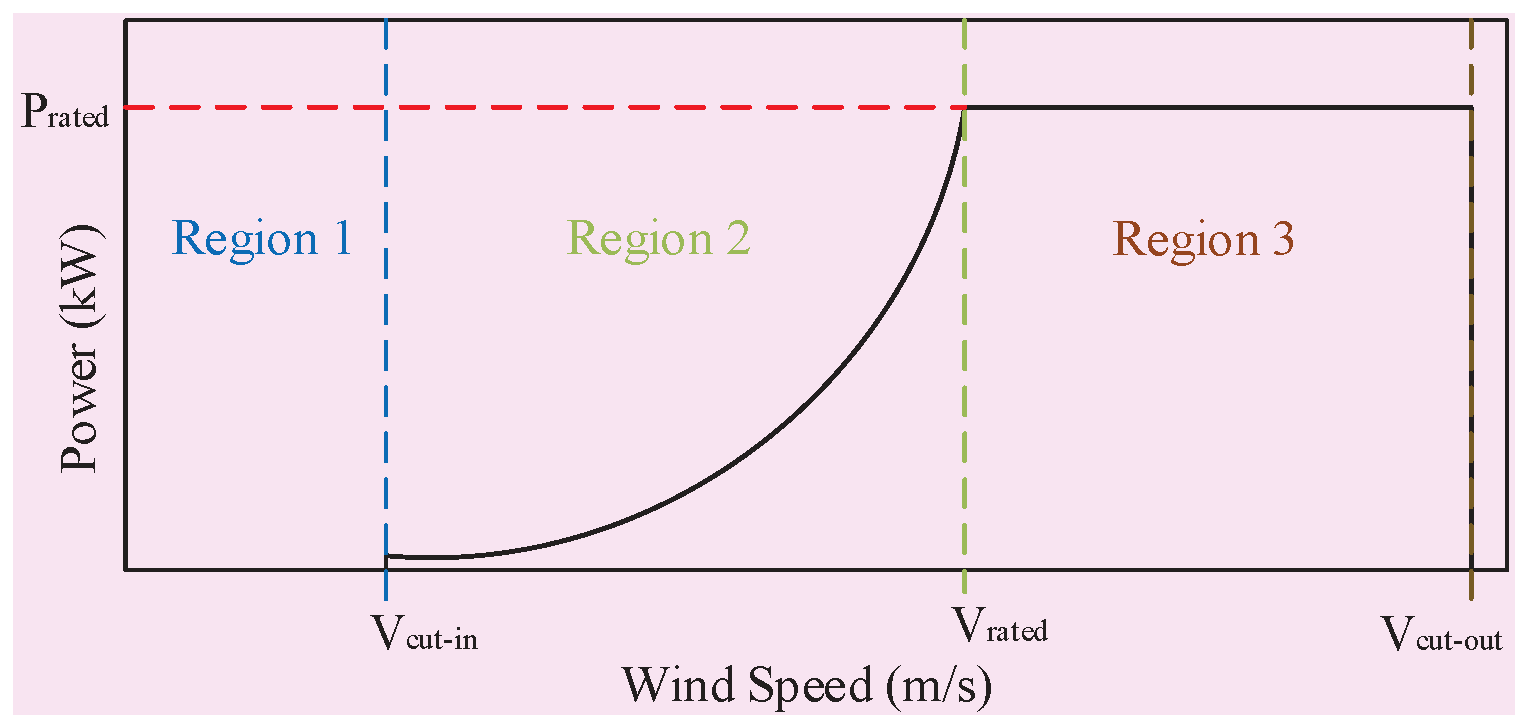
2.2. Aerodynamic Model
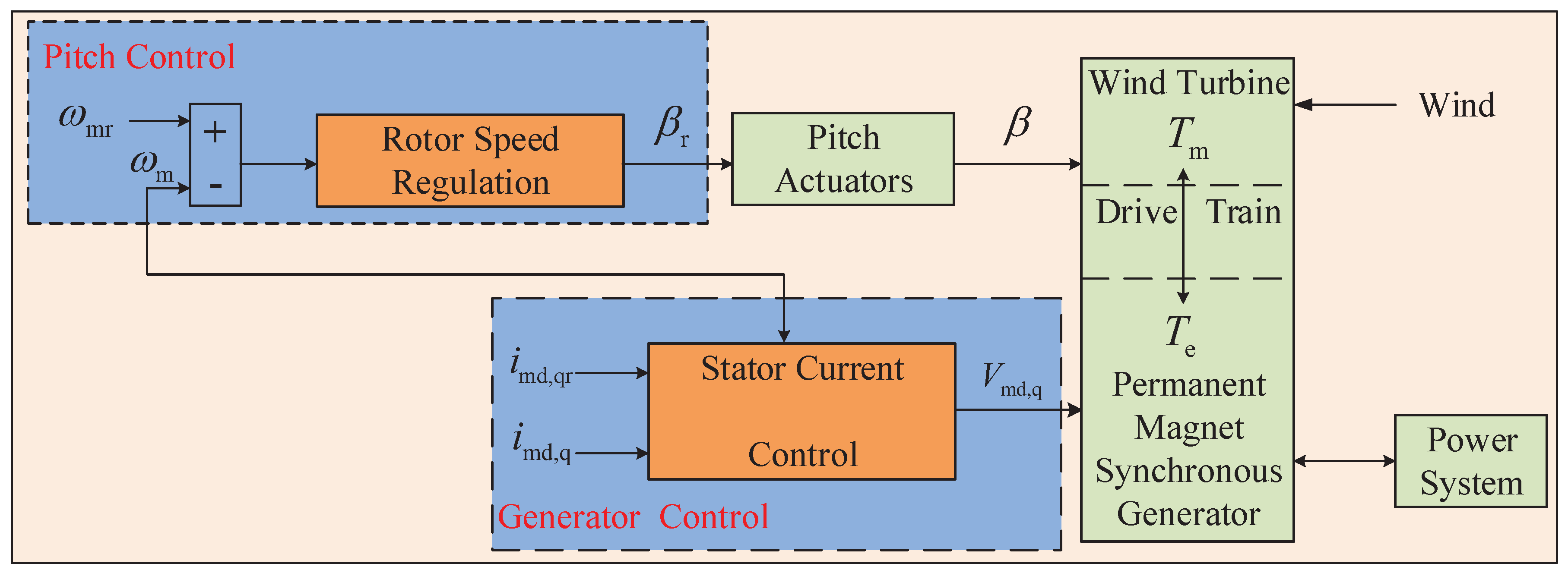
2.3. Pitch Control
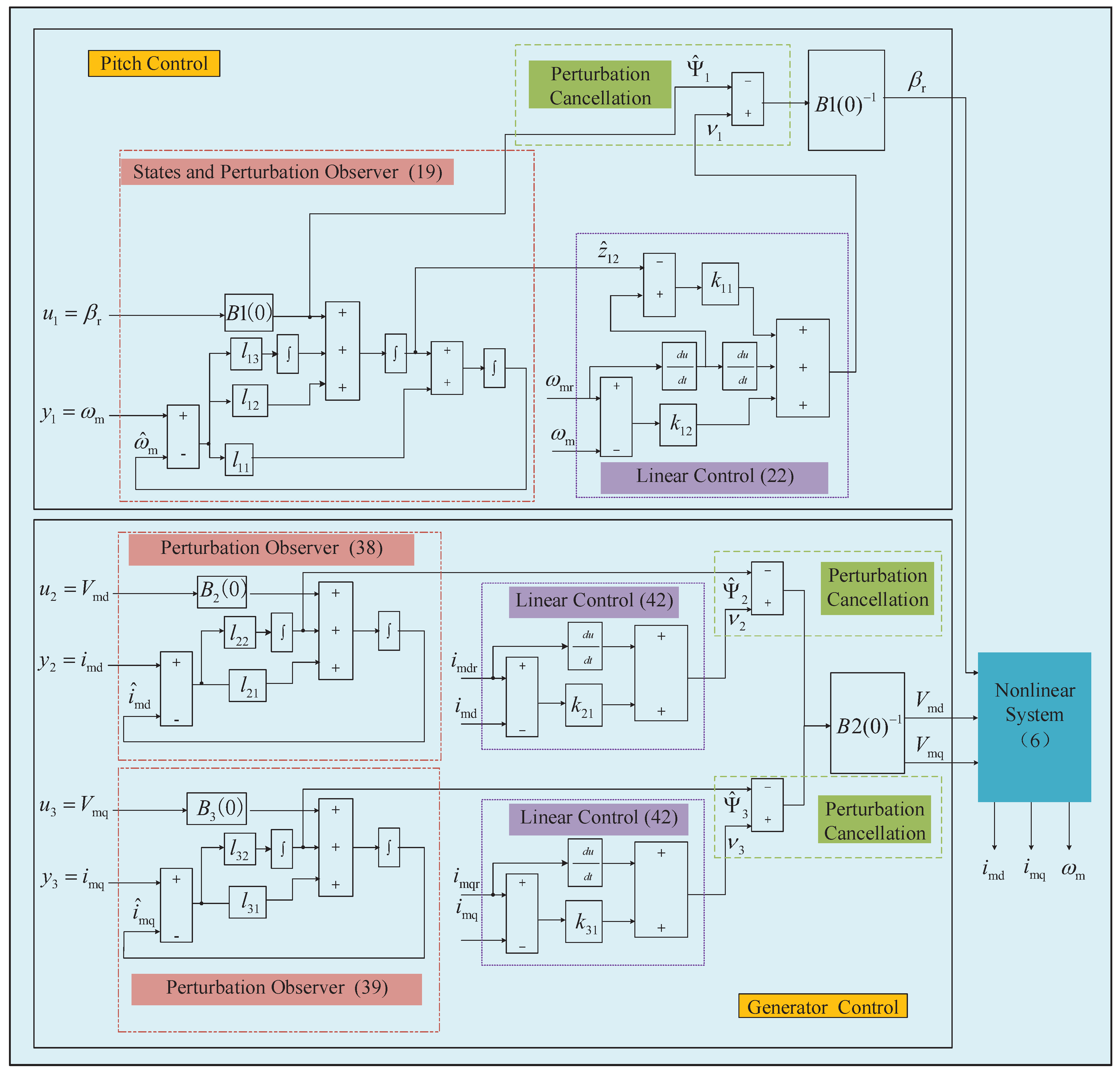
3. Perturbation Observer-Based Nonlinear Adaptive Controller Design
3.1. NAC Design of WT
3.1.1. Input/Output Linearization
3.1.2. Definition of Perturbation and State
3.1.3. Design of States and Perturbation Observer
3.1.4. Design of Nonlinear Adaptive Controller
3.2. NAC Design of PMSG
3.2.1. Input/Output Linearization
3.2.2. Definition of Perturbation and State
3.2.3. Design of Perturbation Observer
3.2.4. Design of Nonlinear Adaptive Controller
3.2.5. Stability Analysis of Closed-Loop System
4. Simulation Results
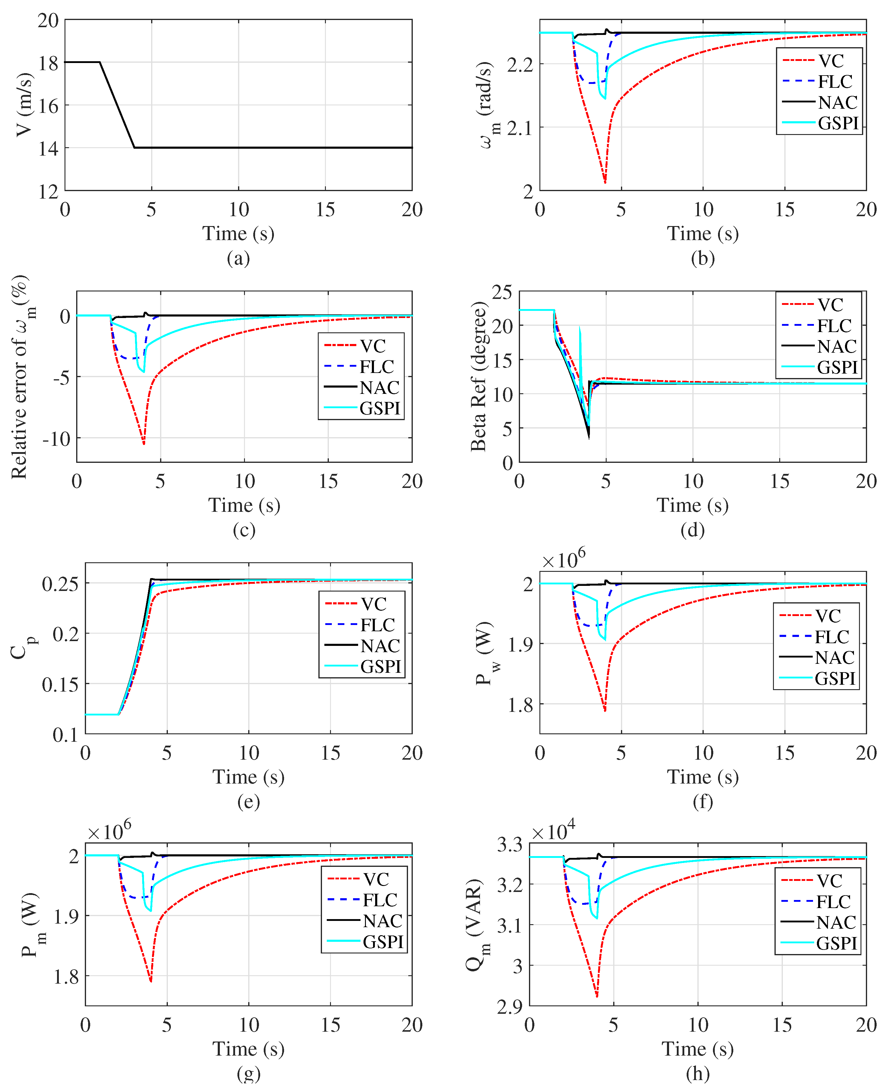
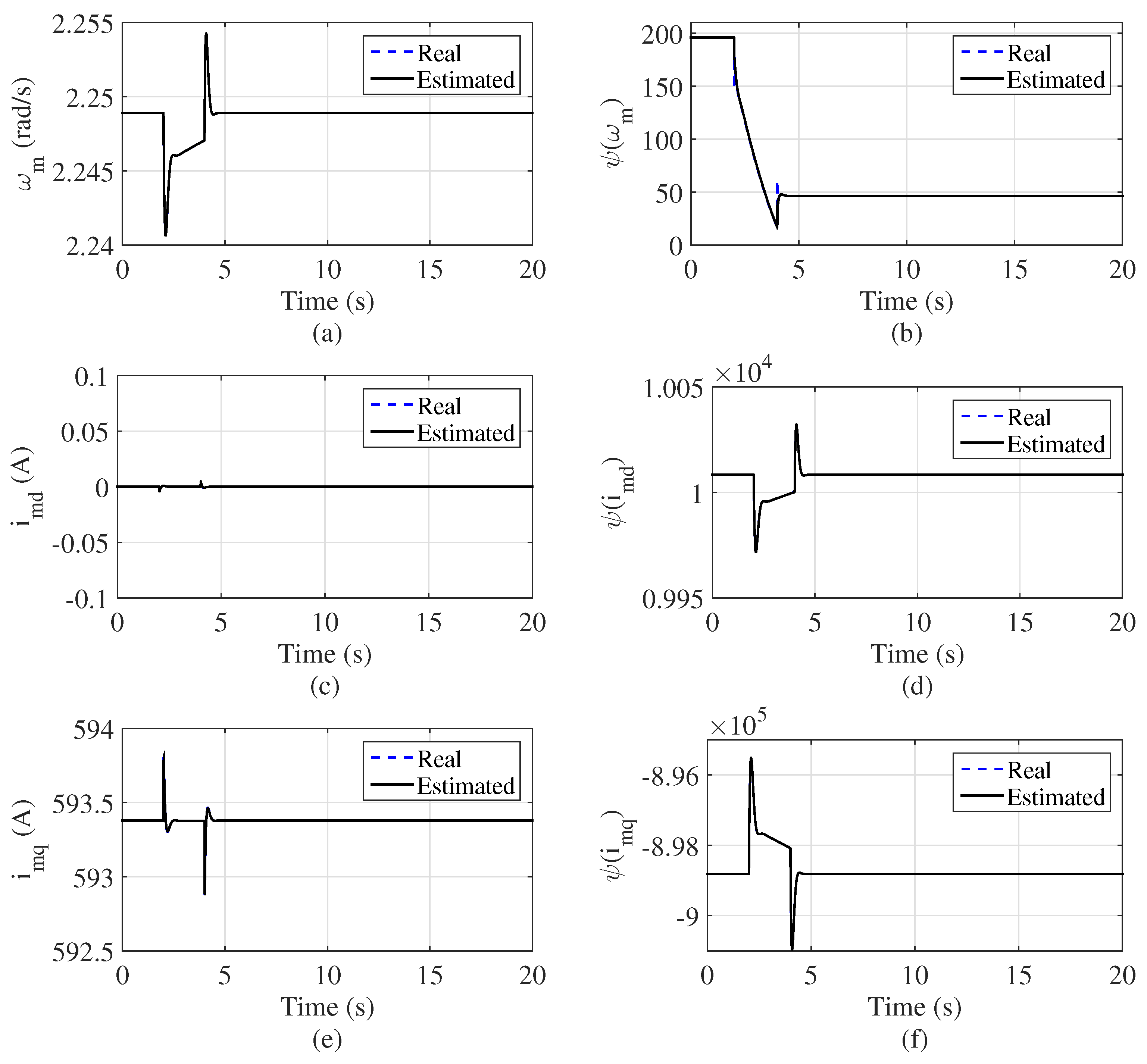
4.1. Ramp Wind
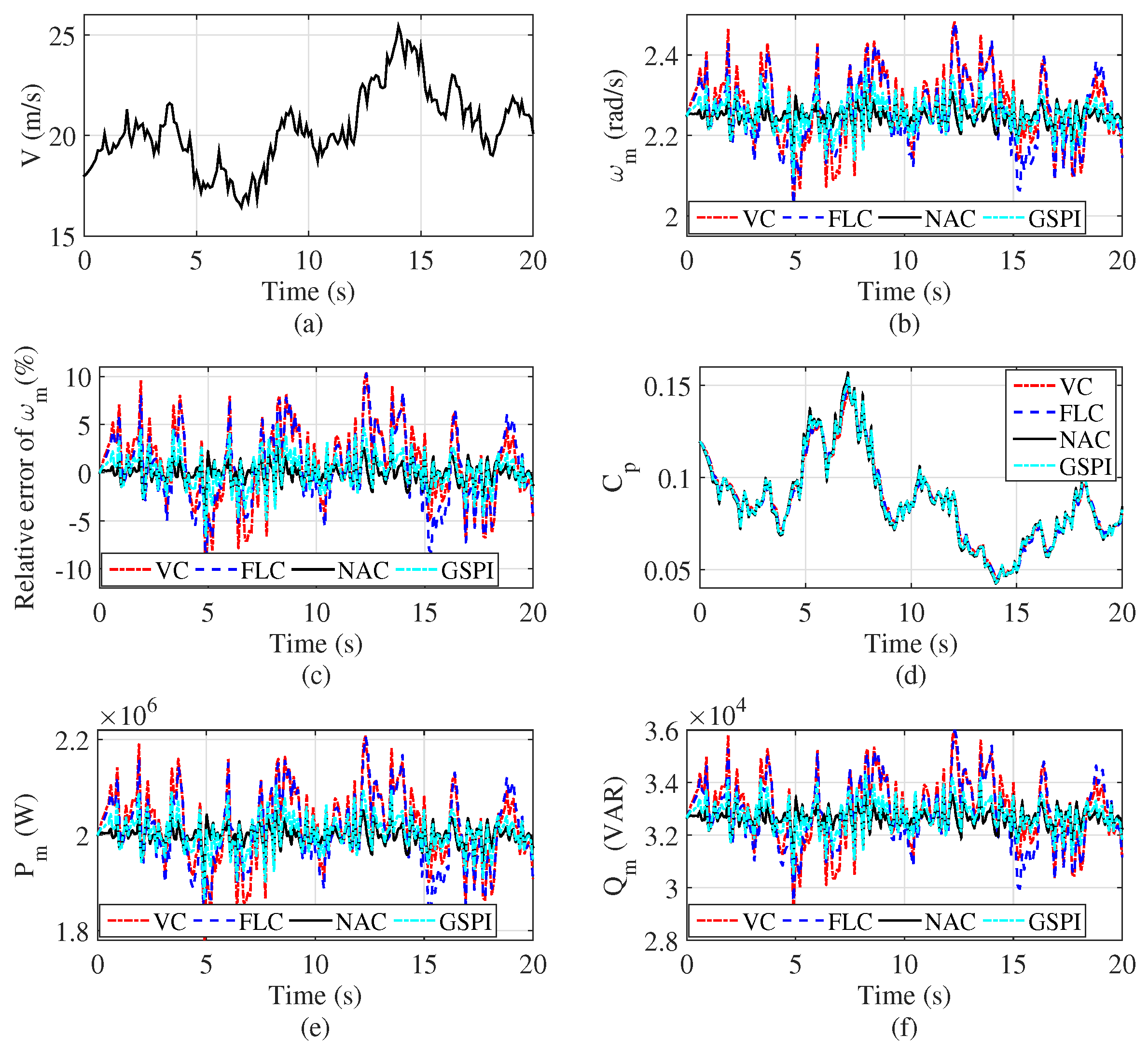
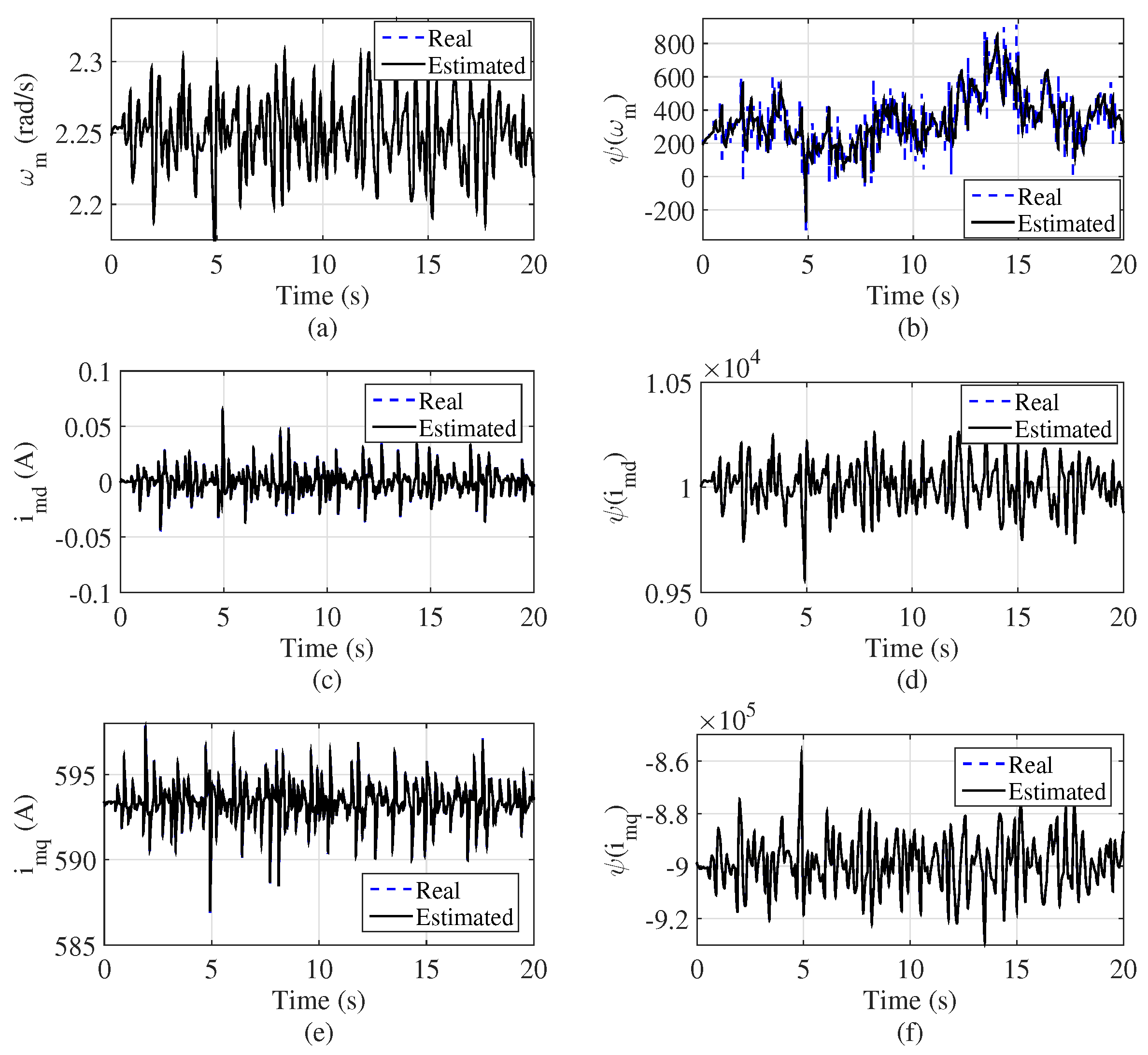
4.2. Random Wind
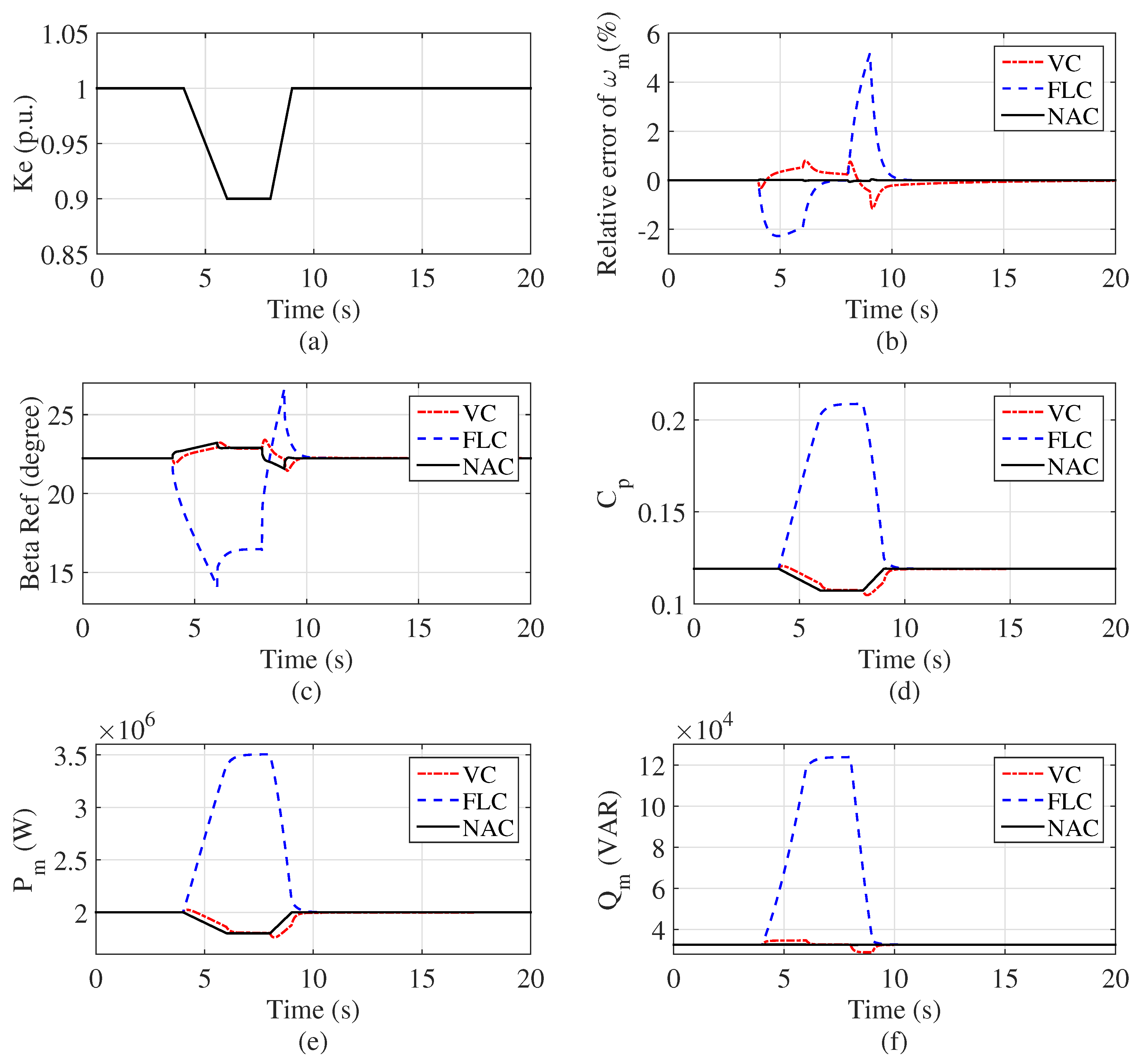
4.3. Robustness Against Parameter Uncertainty
5. Conclusions
Author Contributions
Funding
Conflicts of Interest
References
- Aissaoui, A.G.; Tahour, A.; Essounbouli, A.; Nollet, F.; Abid, M.; Chergui, M.I. A fuzzy-PI control to extract an optimal power from wind turbine. Energy Convers. Manag. 2013, 65, 688–696. [Google Scholar] [CrossRef]
- Chen, J.; Yao, W.; Zhang, C.K.; Ren, Y.X.; Jiang, L. Design of robust MPPT controller for grid-connected PMSG-Based wind turbine via perturbation observation based nonlinear adaptive control. Renew. Energy 2019, 134, 478–495. [Google Scholar] [CrossRef]
- Liao, S.W.; Yao, W.; Han, X.N.; Wen, J.Y.; Cheng, S.J. Chronological operation simulation framework for regional power system under high penetration of renewable energy using meteorological data. Appl. Energy 2017, 203, 816–828. [Google Scholar] [CrossRef]
- Yang, B.; Jiang, L.; Yao, W.; Wu, Q.H. Nonlinear maximum power point tracking control and modal analysis of DFIG based wind turbine. Int. J. Electr. Power Energy Syst. 2016, 74, 429–436. [Google Scholar] [CrossRef] [Green Version]
- Liu, J.; Yao, W.; Wen, J.Y.; Fang, J.K.; Jiang, L.; He, H.B.; Cheng, S.J. Impact of power grid strength and PLL parameters on stability of grid-connected DFIG wind farm. IEEE Trans. Sustain. Energy 2019. [Google Scholar] [CrossRef]
- Yang, B.; Zhang, X.S.; Yu, T.; Shu, H.C.; Fang, Z.H. Grouped grey wolf optimizer for maximum power point tracking of doubly-fed induction generator based wind turbine. Energy Convers. Manag. 2017, 133, 427–443. [Google Scholar] [CrossRef]
- Abdullah, M.A.; Yatim, A.H.M.; Tan, C.W.; Saidur, R. A review of maximum power point tracking algorithms for wind energy systems. Renew. Sustain. Energy Rev. 2012, 16, 3220–3227. [Google Scholar] [CrossRef]
- Kumar, A.; Stol, K. Simulating feedback linearization control of wind turbines using high-order models. Wind Energy 2009, 13, 419–432. [Google Scholar] [CrossRef]
- Boukhezzar, B.; Siguerdidjane, H. Nonlinear Control of a variable-speed wind turbine using a two-mass model. IEEE Trans. Energy Convers. 2011, 26, 149–162. [Google Scholar] [CrossRef]
- Van, T.; Nguyem, T.H.; Lee, D.C. Advanced pitch angle control based on fuzzy logic for variable-speed wind turbine systems. IEEE Trans. Energy Convers. 2015, 30, 578–587. [Google Scholar] [CrossRef]
- Boukhezzar, B.; Lupu, L.; Siguerdidjane, H.; Hand, M. Multivariable control strategy for variable speed, variable pitch wind turbines. Renew. Energy 2007, 32, 1273–1287. [Google Scholar] [CrossRef]
- Connor, B.; Leithead, W.E.; Grimble, M. LQG control of a constant speed horizontal axis wind turbine. Proc. IEEE CCA 1994, 1, 251–252. [Google Scholar]
- Bossanyi, E.A. The design of closed loop controllers for wind turbines. Wind Energy 2000, 3, 149–163. [Google Scholar] [CrossRef]
- Akhmatov, V.; Knudsen, H.; Nielsen, A.H.; Pedersen, J.K.; Poulsen, N.J. Modelling and transient stability of large wind farms. Int. J. Electr. Power Energy Syst. 2003, 25, 123–144. [Google Scholar] [CrossRef]
- Pao, L.; Johnson, K. A tutorial on the dynamics and control of wind turbines and wind farms. Proc. ACC 2009. [Google Scholar] [CrossRef]
- Mullane, A.; Lightbody, G.; Yacamini, R. Wind-turbine fault ride-through ehancement. IEEE Trans. Power Syst. 2005, 20, 1929–1937. [Google Scholar] [CrossRef]
- Seol, J.Y.; Ha, I.J. Feedback-linearizing control of IPM motors considering magnetic saturation effect. IEEE Trans. Power Electron. 2005, 20, 416–424. [Google Scholar] [CrossRef]
- Kim, K.H.; Jeung, Y.C.; Lee, D.C.; Kim, H.J. LVRT strategy of PMSG wind power systems based on feedback linearization. IEEE Trans. Power Electron. 2012, 27, 2376–2384. [Google Scholar] [CrossRef]
- Jiang, L.; Wu, Q.H. Nonlinear adaptive control via sliding-mode state and perturbation observer. IEEE Proc. Control Theory Appl. 2002, 149, 269–277. [Google Scholar] [CrossRef]
- Mauricio, J.M.; Leon, A.E.; Gomez-Exposito, A.; Solsona, J.A. An adaptive nonlinear controller for DFIM-based wind energy conversion systems. IEEE Trans. Energy Convers. 2008, 23, 1024–1035. [Google Scholar] [CrossRef]
- Yang, B.; Yu, T.; Shu, H.C.; Dong, J.; Jiang, L. Robust sliding-mode control of wind energy conversion systems for optimal power extraction via nonlinear perturbation observers. Appl. Energy 2018, 210, 711–723. [Google Scholar] [CrossRef]
- Noureldeen, O.; Hamdan, I. Design of robust intelligent protection technique for large-scale grid-connected wind farm. Prot. Control Mod. Power Syst. 2018, 3, 169–182. [Google Scholar] [CrossRef]
- Shen, Y.; Yao, W.; Wen, J.Y.; He, H.B.; Jiang, L. Resilient wide-area damping control using GrHDP to tolerate communication failures. IEEE Trans. Smart Grid 2019, 10, 2547–2557. [Google Scholar] [CrossRef]
- Han, B.; Zhou, L.W.; Yang, F.; Xiang, Z. Individual pitch controller based on fuzzy logic control for wind turbine load mitigation. IET Renew. Power Gener. 2016, 10, 687–693. [Google Scholar] [CrossRef]
- Liu, J.; Wen, J.Y.; Yao, W.; Long, Y. Solution to short-term frequency response of wind farms by using energy storage systems. IET Renew. Power Gener. 2016, 10, 669–678. [Google Scholar] [CrossRef]
- Saravanakumar, R.; Jena, D. Validation of an integral sliding mode control for optimal control of a three blade variable speed variable pitch wind turbine. Int. J. Electr. Power Energy Syst. 2015, 69, 421–429. [Google Scholar] [CrossRef]
- Saravanakumar, R.; Jena, D. Modified vector controlled DFIG wind energy system based on barrier function adaptive sliding mode control. Prot. Control Mod. Power Syst. 2019, 4, 34–41. [Google Scholar]
- Lin, W.M.; Hong, C.M. A new Elman neural network-based control algorithm for adjustable-pitch variable-speed wind-energy conversion systems. IEEE Trans. Power Electron. 2011, 26, 473–481. [Google Scholar] [CrossRef]
- Chen, J.; Jiang, L.; Yao, W.; Wu, Q.H. Perturbation estimation based nonlinear adaptive control of a full-rated converter wind-turbine for fault ride-through capability enhancement. IEEE Trans. Power Syst. 2014, 29, 2733–2743. [Google Scholar] [CrossRef]
- Chen, J.; Yao, W.; Ren, Y.X.; Wang, R.T.; Zhang, L.H.; Jiang, L. Nonlinear adaptive speed control of a permanent magnet synchronous motor: A perturbation estimation approach. Control Eng. Pract. 2019, 85, 163–175. [Google Scholar] [CrossRef]
- Yang, B.; Yu, T.; Shu, H.C.; Zhang, Y.M.; Chen, J.; Sang, Y.Y.; Jiang, L. Passivity-based sliding-mode control design for optimal power extraction of a PMSG based variable speed wind turbine. Renew. Energy 2018, 119, 577–589. [Google Scholar] [CrossRef]
- Yang, B.; Yu, T.; Shu, H.C.; Zhu, D.N.; Zeng, F.; Sang, Y.Y.; Jiang, L. Perturbation observer based fractional-order PID control of photovoltaics inverters for solar energy harvesting via Yin-Yang-Pair optimization. Energy Convers. Manag. 2018, 171, 170–187. [Google Scholar] [CrossRef]
- Ren, Y.X.; Li, L.Y.; Brindley, J.; Jiang, L. Nonlinear PI control for variable pitch wind turbine. Control Eng. Pract. 2016, 50, 84–94. [Google Scholar] [CrossRef] [Green Version]
- Xia, Y.; Ahmed, K.H.; Williams, B.W. A new maximum power point tracking technique for permanent magnet synchronous generator based wind energy conversion system. IEEE Trans. Power Electron. 2011, 26, 3609–3620. [Google Scholar] [CrossRef]
- Uehara, A.; Pratap, A.; Goya, T.; Senjyu, T.; Yona, A.; Urasaki, N.; Funabashi, T. A coordinated control method to smooth wind power fluctuations of a PMSG-based WECS. IEEE Trans. Energy Convers. 2011, 26, 550–558. [Google Scholar] [CrossRef]
- Jiang, L.; Wu, Q.H.; Wen, J.Y. Decentralized nonlinear adaptive control for multimachine power systems via high-gain perturbation observer. IEEE Trans. Circuits Syst. I Regul. Pap. 2004, 51, 2052–2059. [Google Scholar] [CrossRef]
- Youcef, K.; Wu, S. Input/output linearization using time delay control. J. Dyn. Syst. Meas. Control 1992, 114, 10–19. [Google Scholar] [CrossRef]
- Yang, B.; Jiang, L.; Yao, W.; Wu, Q.H. Perturbation estimation based coordinated adaptive passive control for multimachine power systems. Control Eng. Pract. 2015, 44, 172–192. [Google Scholar] [CrossRef] [Green Version]
- Wu, Q.H.; Jiang, L.; Wen, J.Y. Decentralized adaptive control of interconnected non-linear systems using high gain observer. Int. J. Control 2004, 77, 703–712. [Google Scholar] [CrossRef]


| Parameters | Values | Units |
|---|---|---|
| Air density | 1.205 | |
| Rated wind speed | 12 | |
| Blade radius R | 39 | m |
| Actuator time constant | 1 | |
| pitch angle rate | ±10 | |
| Rated output power | 2 | MW |
| Stator resistance | 50 | |
| d-axis inductance | 5.5 | mH |
| q-axis inductance | 3.75 | mH |
| Number of pole pairs p | 11 | |
| Field flux | 136.25 | |
| Total inertia | 10,000 |
| Parameters of the NAC Equation (41) | |
|---|---|
| Gains of observer Equation (19) | , , , |
| Gains of observer Equation (37) | , , |
| Gains of observer Equation (38) | , , |
| Gains of linear controller Equation (40) | , , , |
| Simulation Scenarios | Variables | Controllers | ||
|---|---|---|---|---|
| VC | FLC | NAC | ||
| Ramp wind speed | 0.817 | 0.1555 | ||
| Random wind speed | 1.369 | 1.273 | ||
| Field flux variation | 0.0695 | 0.207 | ||
| 67.78 | 1957 | 0.04528 | ||
© 2019 by the authors. Licensee MDPI, Basel, Switzerland. This article is an open access article distributed under the terms and conditions of the Creative Commons Attribution (CC BY) license (http://creativecommons.org/licenses/by/4.0/).
Share and Cite
Chen, J.; Yang, B.; Duan, W.; Shu, H.; An, N.; Chen, L.; Yu, T. Adaptive Pitch Control of Variable-Pitch PMSG Based Wind Turbine. Appl. Sci. 2019, 9, 4109. https://doi.org/10.3390/app9194109
Chen J, Yang B, Duan W, Shu H, An N, Chen L, Yu T. Adaptive Pitch Control of Variable-Pitch PMSG Based Wind Turbine. Applied Sciences. 2019; 9(19):4109. https://doi.org/10.3390/app9194109
Chicago/Turabian StyleChen, Jian, Bo Yang, Wenyong Duan, Hongchun Shu, Na An, Libing Chen, and Tao Yu. 2019. "Adaptive Pitch Control of Variable-Pitch PMSG Based Wind Turbine" Applied Sciences 9, no. 19: 4109. https://doi.org/10.3390/app9194109