Multi-Objective Optimal Capacity Planning for 100% Renewable Energy-Based Microgrid Incorporating Cost of Demand-Side Flexibility Management

Abstract

The need for energy and environmental sustainability has spurred investments in renewable energy technologies worldwide. However, the flexibility needs of the power system have increased due to the intermittent nature of the energy sources. This paper investigates the prospects of interlinking short-term flexibility value into long-term capacity planning towards achieving a microgrid with a high renewable energy fraction. Demand Response Programs (DRP) based on critical peak and time-ahead dynamic pricing are compared for effective demand-side flexibility management. The system components include PV, wind, and energy storages (ESS), and several optimal component-sizing scenarios are evaluated and compared using two different ESSs without and with the inclusion of DRP. To achieve this, a multi-objective problem which involves the simultaneous minimization of the loss of power supply probability (LPSP) index and total life-cycle costs is solved under each scenario to investigate the most cost-effective microgrid planning approach. The time-ahead resource forecast for DRP was implemented using the scikit-learn package in Python, and the optimization problems are solved using the Multi-Objective Particle Swarm Optimization (MOPSO) algorithm in MATLAB^®. From the results, the inclusion of forecast-based DRP and PHES resulted in significant investment cost savings due to reduced system component sizing.

1. Introduction

The quest for provision of affordable, clean, and reliable electricity supply is the key aspiration of many nations globally. These aspirations are portrayed by the commitment of most countries to the formulation and chartering of strategic policies that are targeted towards attaining 100% green energy transition in the near future [1]. Many countries have embarked on different sustainable energy pathways; for example Germany [2] and Sweden [3] aims to attain 100% renewable energy by 2050 while Hawaii in the United States has set 2045 as a target [4]. Several African countries have also taken significant steps and shown visible commitment towards massive green energy uptakes mainly by wind and solar energy. Countries such as Kenya [5], Ghana [6], Mauritius [7], Nigeria [8], Egypt, and South Africa [9] are currently making efforts in the integration of renewable energy technologies on both small and large scale. However, the incorporation of variable renewable energy resources (VREs) such as wind and solar energy increases the flexibility needs of a power system. Hence, to achieve an acceptable level of power system operation reliability, dynamic and vibrant control strategies need to be devised to balance the demand and supply using efficient flexibility mechanism [10]. Flexibility providers are, usually, adaptable resources needed to address the short-term mismatches between the instantaneous generated power and the load demand [11].

Most of the classical power system planning strategies comprises of segregated optimization models for power system design. These models generally comprise of three features which are component sizing to determine the optimal capacity configuration, unit commitment model to determine the optimal operation strategy, and electricity market strategies to evaluate optimal point-to-point energy transactions [12]. However, the segregated approach is not sufficient for achieving an optimally reliable system design; this is because the operational efficiency of power system relies highly on the time-based dispatchability and controllability of the system generating resources. Furthermore, with the increasing penetration of VREs, the controllability and dispatchability of power system generation sources becomes more complex. Hence, the planning for the transition towards a high VREs-based energy system requires an integrated system planning that involves the cost of component sizing and system flexibility [13]. A comprehensive investigation of the economic viability of different kinds of flexibility providers available for power systems is discussed in [14]. The cost of flexibility is defined as the additional cost required to integrate additional adaptable resources to address the intermittency of VREs integration. There are many sources of flexibility provider options; these includes system interconnection, demand-side management, supply-side management, storage technologies, etc. [15]. From the generation planning perspective, flexibility is investigated based on the ramping capability of the generators, the minimum possible attainable generation, increased cycles of shutdowns and startups for hybrid configuration as outlined in [16].

The idea of hybrid-energy system has also shown some significant growing interest as a valuable and efficient flexibility provider towards 100% VREs generation as shown in much recent research. The authors in [14] performed and provided a comprehensive framework for techno-economic flexibility analysis based on MILP optimization model by combining complimentary distribution generation alternatives such as thermal storage, heat pump, and cogeneration. The importance of the appropriate selection of complementary generating technologies coupled with energy storage system (ESS), with an improved optimal operation strategy, as a cost-effective path towards ensuring power system flexibility is highlighted in [17]. Electricity storage has played a valuable and significant central role in power system in many aspects [18]. Energy storage has the advantage to time-shift the electrical energy supply thus it acts as an ideal mechanism for moderating the consequences of fluctuating output of VREs on the power system. There are many well-known types of ESS in many works of literature varying in terms of technical and economic specification as summarized in [19]. Many studies have evaluated and demonstrated the cost–benefits of appropriate selection and application of different ESS technologies incorporation into the power system planning. The common ESS ranges from pumped hydro [20], hydrogen storage [21], BESS [22], compressed air energy storage, etc. [23]. The inclusion of demand-side management into optimal component sizing that involves energy storage (ESS) facilities is proposed in [24]. The final outcomes show that using the demand-side management (DSM) increases the system flexibility and offers an economical planning option with reduced ESS capacity requirement.

There are two main categories of end-user electrical demand namely the flexible load demand (FDRs) and inflexible/static load demand. The flexible load demand (FDR) are assumed to be those appliances whose time of use can be transferred from one period to another. FDRs include heat pump, room heater, washing machines, etc. They are also referred to as the shiftable appliances because their usage can be delayed during the period of peak demand or shortage of electricity supply and activated later during the period of over-generation. Non-shiftable load demands, on the other hand, are appliances that are static in terms of the time of use, they have a fixed time of period as to when to use, such as illumination loads. DSM has recently received heightened attention in terms of flexibility provision capability using flexible demand resources (FDRs) to achieve the controllability of the customer load demand pattern [25]. In general, the FDRs provide allowances and capacity for time-shifting in terms of their energy requirements. A proper schedule of the FDRs can guarantee mitigation of the gap that exists between demand and system generation for power systems with very high renewable energy fraction as addressed in [26]. A demand-side flexibility approach using the controllability of FDRs has been developed with a detailed implementation framework for commercial and residential smart building in [27]. Demand response program (DRP) is a subset of DSM designed to influences the consumer’s behaviors in terms of the time of usage of the FDR through motivations such as incentive payments and lucrative electricity prices to improve the overall system efficiency [28]. The concepts of DRP have been adequately covered in the literature with much focus on optimizing the electricity market design. The commonly featured types of DRPs found in the literature includes and not limited to; real-time pricing, day-ahead pricing, time of use, interrupted curtailable, direct load control, critical peak pricing, etc. [29]. Successful implementation of DRP should take into account the current and the forecasted future power system status to fully exploit the market flexibility [30] and captures the VREs generation uncertainties [31,32].

However, an accurate and reliable VREs output forecasting can serve as a core and vital component of energy management systems (EMS) implementation [33]. The role of forecasting also has significant value in the implementation of pricing schemes in the power markets to decrease the rate of market volatility [34]. Hence, power forecasting plays a pivotal role in flexibility planning for integrating and addressing the uncertainty of the VREs in hybrid power systems. Accurate power forecasting provides critical information of the anticipated status (power shortages and surplus) of the power system ahead of time before the actual occurrence. Hence, a good foresight of the time-ahead generation profile provides an opportunity to plan for future uncertainties adequately and cost-effectively. The ability of a system to meet and handle the growing ramping requirements and volatile residual demand is a significant concern of system operators as the share of wind and solar increases. The economic benefit of accurate solar forecasting in minimizing the generation cost, as well as managing power curtailment was investigated and illustrated by Martinez-Anido et al. [32]. A detailed approach has been adopted for wind power forecast application in [35] and in [36] considering several power market scenarios.

1.1. Research Motivation

Various research has been conducted on optimum component sizing using various optimization techniques to evaluate a cost-effective hybrid microgrid configuration such as PV/biodiesel/BESS using simulated annealing [37], Supercapacitors/BESS/WT/Fuel using Non-dominated Sorted Genetic Algorithm [6], diesel/PV/WT using multi-objective self-adaptive differential evolution algorithm [38], PV/WT/BESS using cuckoo search algorithm [39], MOPSO [40], GA-PSO and MOPSO [41], and more. However, it is observed from the research trends in the literature that in order to ascertain the maximum techno-economic benefits for any microgrid configuration and investment, the flexibility requirements of the system must be factored into its design, i.e., reliability based on adequate system flexibility provision must be prioritized alongside the planning and capacity sizing. Hence, in this study, a multi-objective optimal planning for an isolated microgrid that introduces the cost of flexibility management using ESS and DRP is investigated. The multi-objective design problem is formulated and solved using the Multi-Objective Particle Swarm Optimization (MOPSO) algorithm in MATLAB environment.

1.2. Research Contribution

In view of the above, the main contribution of this work is to introduce a suitable cost-effective framework for incorporating short-term flexibility management requirements into the long-term planning of renewable energy-based microgrid. The total cost of investment and flexibility management, and the supply reliability requirements are investigated and compared under different system design scenarios using the multi-objective optimization approach. The effectiveness of ensembled data-driven renewable energy generation forecasting using the Gradient Boosted regression trees (GBRT) techniques for DSM/DRP flexibility planning and efficient coordination of FDRs is analyzed and compared with the critical peak pricing DRP alternative. The economic advantage of using PHES, compared to BESS, in microgrid applications that requires high renewable energy fraction has been demonstrated through simulation using the data for a real Kenyan microgrid case study.

The rest of the paper is organized as follows; Section 2 presents the methodology and system modeling, Section 3 provides an overview of the FDR, and the techniques of each DRP is described. The optimization problems are formulated in Section 4 while Section 5 provided the details of the case study and simulation parameters, simulation results are outlined and discussed in Section 6 and finally, Section 7 provides the conclusion of the work.

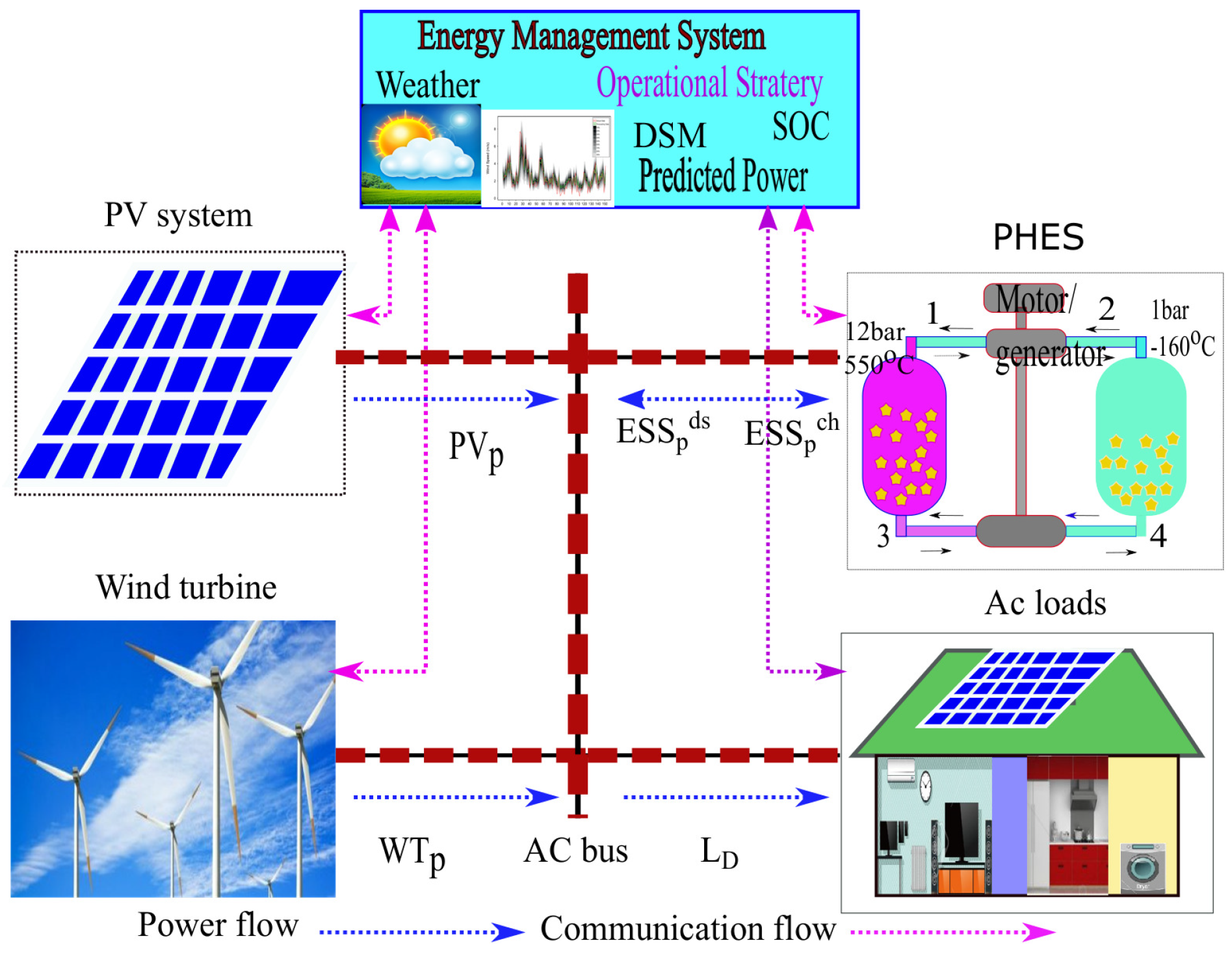
2. Methodology and System Modeling

Figure 1 shows the proposed microgrid system infrastructure; which consist of the WT, PV, PHES, and AC loads connected through an AC bus. The energy management system is also included as the control center for the microgrid. The mathematical models that describe the behavior of each system component and the energy management strategies deployed in this study are discussed below.

2.1. Wind Turbine

The output power of a wind generator $W{T}_P\left(t\right)$ is a function of wind speed and can be calculated using Equation (1) [42]:

$$W{T}_p\left(t\right)=\left\{\begin{array}{cc}W{T}_p^{rtd}\left(t\right)\times \frac{u^3-u_{in}^3}{u_{rtd}^3-u_{ou}^3}\hfill & u_{ci}\le u\le u_{rtd}\hfill \\ W{T}_p^{rtd}\left(t\right)\hfill & u_{rtd}\le u\le u_{ou}\hfill \\ 0\hfill & u<u_{in}\mathrm{or}u>u_{ou}\hfill \end{array}\right.$$

(1)

where $u_{ci}$, $u_{rtd}$, u and $u_{ou}$ are the cut-in speed, nominal speed, instantaneous wind speed at hub height and cut-out wind speed for the wind turbine, respectively. $W{T}_p^{rtd}$ is the rated power output of the wind turbine.

2.2. PV System

The generated output power of the PV system ($P{V}_p\left(t\right)$) is significantly determined by the solar irradiances incident on the PV surface and temperature. The PV output power as a function of input variables is given by (2) [43]:

$$P{V}_p\left(t\right)=f_{pv}\times \frac{G\left(t\right)}{G_{std}}\times [1+{\theta }_i(t_{pv}\left(t\right)-t_{std})]\times P{V}_p^{rtd}$$

(2)

where $f_{pv}$, $P{V}_p^{rtd}$, $G\left(t\right)$ is the power reduction factor, installed capacity of the PV in kW and the incident solar irradiance, respectively. ${\theta }_t$, $G_{std}$, $t_{std}$ is the temperature coefficient, solar irradiance, and temperature under the standard test condition.

2.3. Energy Storage System Model

Whenever the combined output power of WT and PV generation surpasses the capacity of load demand, the ESS transitions into the charging state. The amount of energy stored at any given time t is primarily determined by the difference between the sum of the total PV and WT generation, and the load demand.

2.3.1. Battery Energy Storage System (BESS)

The amount of discharging and charging power drawn or sent to the battery energy storage system, respectively, is subject to the previous state of charge (SOC) as well as the ESS system constraints. The SOC at any given t is determined by the following equation.

$$SOC\left(t\right)=\left[(P{V}_p\left(t\right)+W{T}_p\left(t\right))-\frac{L_D\left(t\right)}{{\beta }_c}\right]\times {\beta }_{ch}+SOC(t-1)\left(1-dr\right)$$

(3)

where $SOC(t-1)$ and $SOC\left(t\right)$ and is the BESS state of charge for the previous and current period in kWh, respectively. $L_D\left(t\right)$ is the load demand, ${\beta }_c$ denotes the power converters efficiency, $dr$ and ${\beta }_{ch}$ is the hourly self-discharge rate and BESS charging efficiency respectively. Whenever the total generation cannot meet the load demand, BESS shifts into the discharging mode. Consequently, the current state of charge at any given time t is given by:

$$SOC\left(t\right)=\left(\frac{L_D\left(t\right)}{{\beta }_{ds}}-(P{V}_p\left(t\right)+W{T}_p\left(t\right))\right)/{\beta }_{ds}+\left(SOC(t-1)\left(1-dr\right)\right)$$

(4)

where ${\beta }_{ds}$ is the discharging efficiency. The energy storage level (SOC) must be constrained within the upper $SO{C}_{max}$ and the lower $SO{C}_{min}$ bounds of the BESS.

$$SO{C}_{min}\le SOC\left(t\right)\le SO{C}_{max}$$

(5)

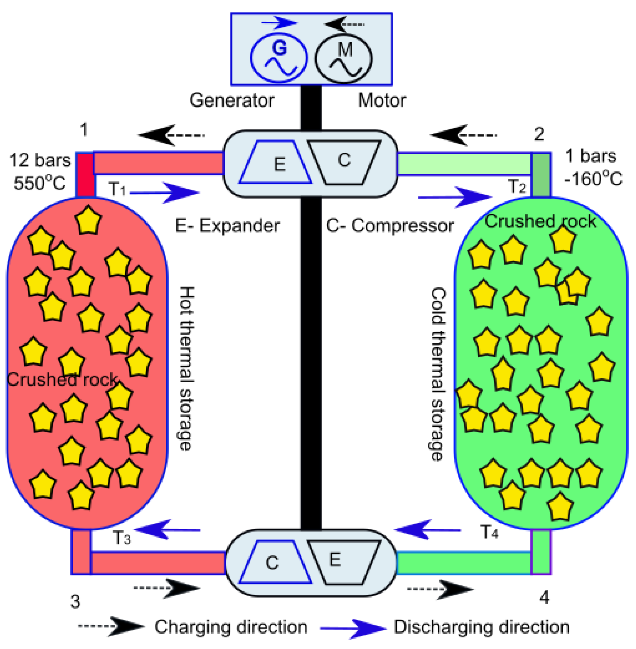
2.3.2. Pumped Heat Energy Storage (PHES)

The PHES stores electricity as sensible heat in two thermal storage system; a hot high pressure and temperature tank (+500 ${}^{\circ }$C, 12 bars pressure) and a cold low pressure and temperature tank (−160 ${}^{\circ }$C, 1 Bar). It also consists of a two compressor/expander pair, argon as a working fluid and it uses gravel as the storage medium. The operation strategy is analogous to pumped hydro storage but rather than pumping water, heat pumping is used to create temperature difference. Theory of operation and development is adequately covered in [44,45,46]. Figure 2. shows the schematic diagram of the PHES.

The energy stored in a PHES depends on the temperature differences between the two thermal storage system. The energy stored $ES{S}_{phes}\left(t\right)$ in the reservoirs per unit volume is the difference between the internal energies of the storage medium in the hot and cold stores. The internal energies of the storage medium are the function of the mass ($M_r$) and specific heat densities of the storage medium ($S{H}_r$). The energy stored can be determined by the temperature difference between the hot and cold store [47] as illustrated below:

$$ES{S}_{phes}\left(t\right)=M_r\times S{H}_r\times \left\{(T_2\left(t\right)-T_3\left(t\right))-(T_1\left(t\right)-T_4\left(t\right))\right\}$$

(6)

The power output and input $P_{phes}\left(t\right)$ of the PHES per unit volume (for charging and discharging instance) is determined by the mass ($Mg$) and the specific heat of the argon gas ($SHg$), and the temperature difference [48] as follows:

$$P_{phes}\left(t\right)=M_g\times S{H}_g\times \left\{(T_2\left(t\right)-T_1\left(t\right))-(T_3\left(t\right)-T_4\left(t\right))\right\}$$

(7)

where $(T_1\left(t\right)$, $T_2\left(t\right))$ are the top and $(T_3\left(t\right)$, $T_4\left(t\right))$ are the bottom section temperature of the hot tank and cold tank respectively.

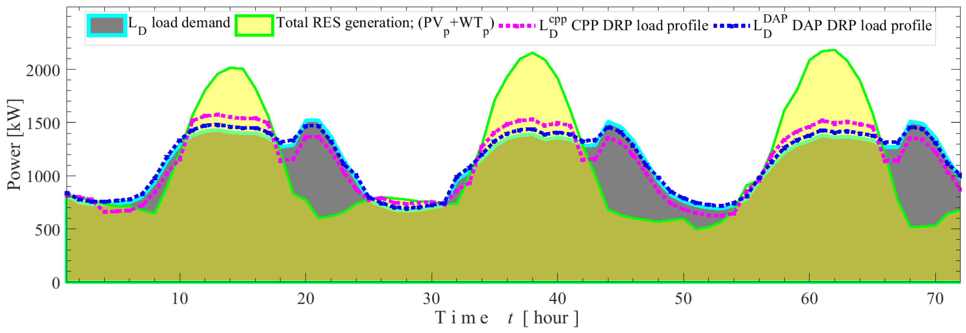
3. Flexible Demand Resources (FDRs) and Demands Response Program (DRPs)

Figure 3 shows the flowchart for the integrated system planning method considered in this work. The framework combines the optimal ESS scheduling and optimal DRP implementations. The FDRs play significant roles in the flexibility management of the system whenever they are appropriately activated to minimize the mismatch between generation and demand. The DSM approach that is employed in this study for the DRPs is based on the optimal scheduling of appropriate FDRs in the microgrid as explained below. The net capacity of the shiftable load demand ($FDR$), throughout the system scheduling period, is assumed to have a maximum range of up to 10% up ($FD{R}^{max}$) and down ($FD{R}^{min}$) of the initial total FDR load demand value [49].

$$FD{R}^{min}\le FDR\left(t\right)\le FD{R}^{max}$$

(8)

3.1. Price Elasticity of Demand and Load Modeling

A change in price of a service will have an impact on the amount of quantity demanded. For instance, a change in the price of electricity ($\partial E_{std}^{pr}\left(i\right)$) in the ith period will result in a change of the load demand ($\partial L_D\left(j\right)$) in the jth period either by increasing or decreasing the load demand. Thus, a change in electricity price during the single period ith affects the load demand during all the periods (T). The price elasticity of demand ($P{E}_{\varphi (i,i)}$) gives a measure of the responsiveness at which the end-user time-shift their energy consumption patterns with respect to change in electricity as shown below:

$$P{E}_{\varphi (i,i)}=\frac{E^{pr}\left(i\right)}{L_D\left(i\right)}.\frac{\partial L_D\left(i\right)}{\partial E^{pr}\left(i\right)};\forall i,j\in T$$

(9)

The price elasticity of demand entails self and cross-elasticity; the self-elasticity defines the sensitivity of load demand with respect to price within the same pricing interval (single period elasticity) and usually has a negative value implying some proportion of the load cannot be transferred from one period to another. On the other hand, cross-elasticity ($P{E}_{\varphi (i,j)}$) defines the load demand sensitivity of the (ith) pricing period in response to the electricity price variation in the (jth) pricing period (multi-period elasticity) and usually has positive value implying some proportion of the load demand is shiftable to another period. The cross-elasticity of load demand is given by [50];

$$P{E}_{\varphi (i,j)}=\frac{E_{std}^{pr}\left(i\right)}{L_D\left(j\right)}.\frac{\partial L_D\left(j\right)}{\partial E^{pr}\left(i\right)};\forall i,j\in T$$

(10)

3.2. Critical Peak Pricing (CPP) Demand Response Program

CPP is a time-based DRP that divide electricity usage time into periods and presents the fixed electricity prices for each period in advance; peak and off-peak periods. It is usually employed to increase system energy efficiency and alleviate stress on the power system especially when the load demand is likely to surpass the generation capacity. It commonly enforces a very high electricity price during system peak load demand periods and for some specific time periods in order to achieve load reduction during these periods, and retains a flat pricing scheme or a lower electricity price during off-peak periods [51]. The electricity customer responds by shifting load demand from one time period to another due to the enforced pricing scheme. The ultimate customer’s demand profile after implementation of CPP DRP is expressed as [41,52]:

$$\begin{array}{c}\hfill L_D^{cpp}\left(i\right)=L_D\left(i\right)\left\{1+P{E}_{\varphi (i,i)}\frac{[E_{cpp}^{pr}\left(i\right)-E_{std}^{pr}\left(i\right)+pd\left(i\right)+ps\left(i\right)]}{E_{std}^{pr}\left(i\right)}\right.\\ \hfill \left.+\sum _{j=1,j\ne i}^{T}P{E}_{\varphi (i,j)}\frac{[E_{cpp}^{pr}\left(j\right)-E_{std}^{pr}\left(j\right)+pd\left(j\right)+ps\left(j\right)]}{E_{std}^{pr}\left(j\right)}\right\}\end{array};\mathrm{for}\mathrm{all}i,j\in T$$

(11)

where $E_{std}^{pr}\left(i\right)$ is the standard Kenyan electricity price before CPP DRP implementation, $E_{cpp}^{pr}\left(i\right)$, $E_{cpp}^{pr}\left(j\right)$ is the electricity price for current ith period and the jth period after implementation of CPP DRP, $pd\left(i\right)$ and $pd\left(j\right)$ are the incentives and $ps\left(i\right)$ and $ps\left(j\right)$ are penalties enforced for non-compliance’s of DRP.

3.3. Time-Ahead Dynamic Pricing (TADP) Demand Response Program

The cost of generation and the corresponding cost of electricity are highly affected by the shortages and surplus of power generated in the power system. Short periods of mismatch in load demand and generation might necessitate an over-sizing or additional capacity in the ESS that might not be necessary or efficiently used during normal operating times. A remedy to this challenge is to offer motivating electricity prices to influence a time shift in FDRs by the end user. A longer pricing horizon ahead of time can guarantee end-user participation in the DRP. Thus, in TADP DRP, time-ahead electricity pricing profile formulated as a function of the mismatch in the forecasted demand and generated power is relayed to the end user an hour (one period) in advance.

3.3.1. Time-Ahead Dynamic Pricing Model

The electricity price for the next hour ($E_{TADP}^{pr}(t+1)$) is determined based on the difference between forecasted total generation output power from renewable energy sources (PV and WT) and the load demand ${\widehat{L}}_D(t+1)$ using the following equation:

$$E_{TADP}^{pr}(t+1)=E_{std}^{pr}(t+1)\left(1+\frac{{\widehat{L}}_D(t+1)-({\widehat{WT}}_p(t+1)+{\widehat{PV}}_p(t+1))}{{\widehat{L}}_D(t+1)}\right)$$

(12)

where ${\widehat{PV}}_p(t+1)$ and ${\widehat{WT}}_p(t+1)$ represent the forecasted generation output power from the PV and WT, respectively. $E_{std}^{pr}(t+1)$ is the initial (standard) Kenyan electricity price initially present for hour $t+1$ before TADP DRP implementation. $E_{TADP}^{pr}(t+1)$ is the next hour electricity price after the implementation of TADP DRP.

3.3.2. Time-Ahead Dynamic Pricing Demand Response Program Load Modeling

The electricity price determined one hour ahead of time for a specific period is the actual price that would be adopted for that period. Based on the electricity price relayed in advance, the end-consumers are either motivated/discouraged to shift their FDRs. The final economic load model after the TADP DRP is implemented is expressed as:

$$\begin{array}{c}\hfill L_D^{TADP}\left(i\right)=L_D\left(i\right)\left\{1+P{E}_{\varphi (i,i)}{\displaystyle \frac{[E_{TADP}^{pr}\left(i\right)-E_{std}^{pr}\left(i\right)+pd\left(i\right)+ps\left(i\right)]}{E_{std}^{pr}\left(i\right)}}\right.\\ \hfill \left.+\sum _{j=1,j\ne i}^{T}P{E}_{\varphi (i,j)}{\displaystyle \frac{[E_{TADP}^{pr}\left(j\right)-E_{std}^{pr}\left(j\right)+pd\left(i\right)+ps\left(j\right)]}{E_{std}^{pr}\left(j\right)}}\right\}\end{array};\mathrm{for}\mathrm{all}i,j\in T$$

(13)

where $E_{std}^{pr}\left(i\right)$ is the current (ith period) Kenyan electricity price before TADP DRP implementation.

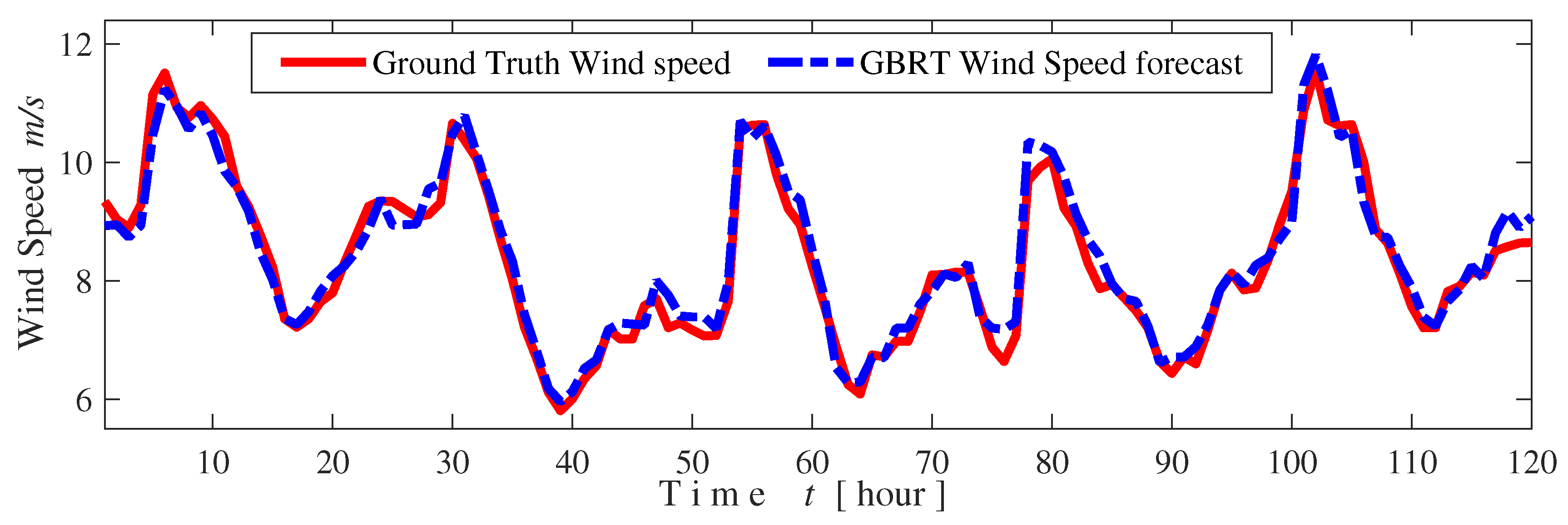
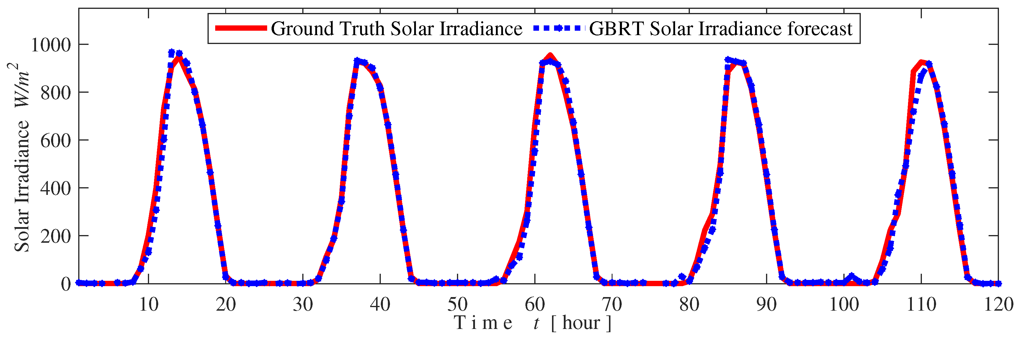
3.3.3. Gradient Boosted Regression Trees (GBRT) Model for Time-Ahead Forecast of Generation

In this work, the forecasting tasks are treated as regression problems and machine learning regression algorithms on scikit-learn package in Python are adopted to build the models using the Gradient boosted regression trees (GBRT) algorithm. The GBRT algorithm has a superior advantage of not requiring complex data pre-processing of dimension transformations or reduction and does not suffer any loss of input variable interpretation [53]. The significant feature of the accurate implementation of the GBRT algorithm is the parameter ${\alpha }_{gbr}$ called the learning rates. The learning rate is a scaling parameter that determines the individual contribution of each decision tree to the final ensemble model. The accuracy of the model is continuously improved by fitting the residual decision iteratively until the desired model is obtained for the best learning rate. Algorithm 1 illustrates the GBRT pseudo code algorithm.

Algorithm 1: Gradient boosted regression trees (GBRT) pseudo code algorithm.

Start: 1.  Precondition: Input the training data set $M=(m_i,o_i)$;$i=1..n$ and                    a differentiate loss function $L_f(o_i,\tilde{o})$ 2. Initialization: Initialize the model with a constant value: $$F_0\left(m\right)=argmin{\sum }_N^{i=1}{L}_f(o_i,\tilde{o})$$ 3.  Estimation:     for $i=1...k$; grow k trees                   (i)   Calculate the Pseudo residuals;                      $$r_{ik}=-{\left[\frac{\partial L_f(o_i,\tilde{o})}{\partial F\left(m_i\right)}\right]}_{F\left(m\right)=F\left(m_i\right)}i=1..n$$                   (ii)  Fit a residual value regression decision tree $I\left(m\right)$                         and establish the terminal leaves                    for     $J=1...j_K$; determine the output of each leaves                           that minimizes; $${\tilde{o}}_{jk}=argmin{\sum }_{m_iϵR_{ij}}{L}_f(o_i,F_{k-1}\left(m_i\right)+\tilde{o})$$ 4.  Update: $$F_k\left(m\right)=F_{k-1}\left(m\right)+{\alpha }_{gbr}{\sum }_{j=1}^{j_k}{\tilde{o}}_{jk}I\left(mϵR_{jm}\right)$$ End: For 5.  Output $F_k\left(m\right)$ End: Terminate the Algorithm

In order ascertain the accuracy of forecasting algorithms, three performance evaluation metrics are used: Mean Absolute Error (MAE), Root mean squared error (RMSE) and Coefficient of Determination ($r^2$).

4. Optimal Design Problem Formulation

The multi-objective optimal design model is evaluated in terms of economic and reliability criteria as presented in the objective functions defined below:

4.1. Economic Criteria: Total Life-Cycle Cost (TPC)

The objective function of the economic criterion is formulated as a cost minimization problem of the net present value of the total life-cycle costs (TPC) of all system components alongside the implementation of the flexibility requirements under different system scenarios. The decision variable of the optimization problem is the capacity of the WT ($C_{WT}$), PV ($C_{PV}$) and ESS ($C_{ESS}$).

$$\mathrm{minimize}TPC=\sum _{z=1}^Z\left\{C{I}_z+\sum _{n=1}^{n=N}\frac{\left(O\&M_z+R{P}_z-R{V}_z\right)}{{(1+r)}^n}\right\}\times C_z$$

(14)

where z indexes the $z_{th}$ component and $C_z$ is the decision variables that represent the optimum component capacities of each of the system components (PV, ESS, and WT). The $TPC$ components are the capital costs ($C{I}_z$), yearly operation and maintenance costs ($O\&M_z$), replacement costs ($R{P}_z$) and the salvage value $R{V}_z$, N is the project lifetime, n is the time step in the project life, i.e., a year and r is the discount rate. The system components have a yearly operation and maintenances cost over the project lifetime.

4.2. Reliability Criteria: Loss of Power Supply Probability (LPSP)

The second objective considers the loss of power supply probability as the system reliability criteria. $LPSP$ reliability index measures and ascertains the quality and reliability performance of the power system design under the different scenarios considered in this study. $LPSP$ is defined as the ratio of the sum of all energy deficits ($LPS$) to the total power demand. Thus, $LPSP$ can be evaluated by using the following expression:

$$LPSP=\frac{{\sum }_{t=1}^{T}LPS\left(t\right)}{{\sum }_{t=1}^T{L}_D\left(t\right)}$$

(15)

where

$$LPS\left(t\right)=L_D\left(t\right)-\left[W{T}_p\left(t\right)+P{V}_p\left(t\right)+\left(SOC(t-1)-SO{C}_{min}\right)\times {\beta }_c\right]$$

(16)

$LPSP$ value ranges between zero and one; a value of 0 for $LPSP$ implies that the load demand will always be met or satisfied, and this is the most desired and preferred performance. The following system $DRP$ constraints are considered during the optimization procedure, alongside the other system component constraints that are mentioned at each design stage.

$$\begin{array}{c}\hfill \begin{array}{c}P{V}_p\left(t\right)+W{T}_p\left(t\right)+ES{S}_p^{ds}\left(t\right)-ES{S}_p^{ch}\left(t\right)=L_D\left(t\right);\mathrm{without}\mathrm{DRP}\hfill \\ P{V}_p\left(t\right)+W{T}_p\left(t\right)+ES{S}_p^{ds}\left(t\right)-ES{S}_p^{ch}\left(t\right)=L_D^{CPP}\left(t\right);\mathrm{with}\mathrm{CPP}\mathrm{DRP}\hfill \\ P{V}_p\left(t\right)+W{T}_p\left(t\right)+ES{S}_p^{ds}\left(t\right)-ES{S}_p^{ch}\left(t\right)=L_D^{TADP}\left(t\right);\mathrm{with}\mathrm{TADP}\mathrm{DRP}\hfill \end{array}\end{array}$$

(17)

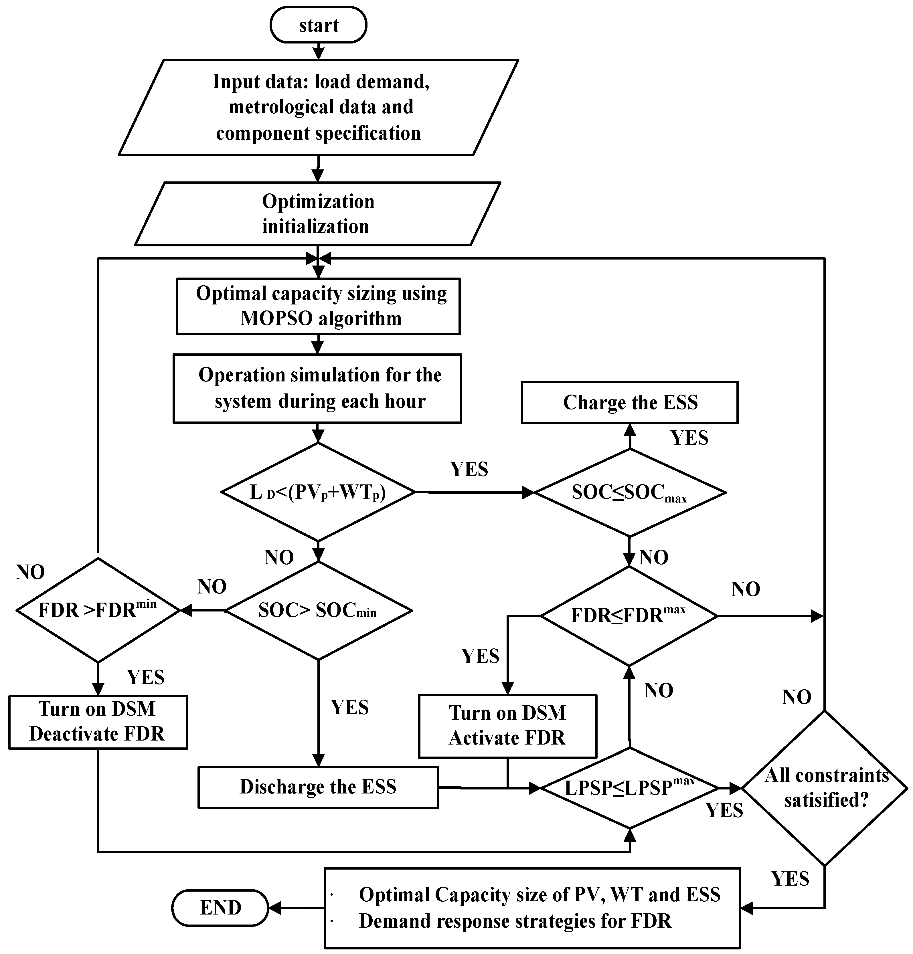
4.3. Overview of the Optimization Tool: Multi-Objective Particle Swarm Optimization

PSO is a population-based approach for solving discrete and continuous optimizations problem that stemmed from and mimic the navigation behavior of swarms of bees, flocks of birds, and schools of fish. To obtain the optimal value of the objective function at each search, two different solution points are obtained which are called the local best, $Pbes{t}_i=(p_{i1},p_{i2},...,p_{id})$ and the global best, is $Pbes{t}_g=gbest=(p_{g1},p_{g2},...,p_{gd})$; and the positions of the particles for the next objective function evaluation is estimated as given below:

$$\begin{array}{c}\hfill V_{id}^{t+1}=w\times v_{id}^k+c_1\times ran{d}_1\times (Pbes{t}_{id}-X_{id})\end{array}$$

(18)

$$\begin{array}{c}\hfill +c_2\times ran{d}_2\times (gbes{t}_d-X_{id})\end{array}$$

(19)

$$X_{id}^{k+1}=X_{id}^k+V_{id}^{k+1}$$

(20)

$$w=w_{damp}\times \frac{ite{r}_{max}-iter}{ite{r}_{max}}+w_i$$

(21)

$iter$ is the iteration count, $ite{r}_{max}$ is the total iterations. $w_i$, $w_f$ are the minimum and maximum range of the inertia weight. The multi-objective PSO approach adopted in this work is described [54]. The repository particles guides the search within the efficient, non-inferior and admissible pareto front by sorting out the non-dominated solutions. The exploratory capacity of the algorithm is strengthened by a special mutation operator just like in NSGA II algorithm as explained below. If $\overrightarrow{f}\left(\overrightarrow{x}\right)$ consists of n objective functions each with m decision variables, then the multi-objective problem can be defined as finding the vector ${\overrightarrow{x}}^{*}={[x_1^{*},x_2^{*},...,x_m^{*}]}^T$ which minimizes $\overrightarrow{f}\left(\overrightarrow{x}\right)$ as shown:

$$\begin{array}{c}\hfill \mathrm{minimize}\overrightarrow{f}\left(\overrightarrow{x}\right)=[f_1\left(\overrightarrow{x}\right),f_{\overrightarrow{2}}\left(x\right),...f_n\left(\overrightarrow{x}\right)]\mathrm{for}{\overrightarrow{x}}^{*}\in \epsilon \end{array}$$

(22)

$$\begin{array}{c}\hfill \overrightarrow{g}\left(\overrightarrow{x}\right)\le 0\end{array}$$

(23)

$$\begin{array}{c}\hfill \overrightarrow{h}\left(\overrightarrow{x}\right)=0\end{array}$$

(24)

$\overrightarrow{g}$ and $\overrightarrow{h}$ are sets of inequality and equality constraints, respectively. A point ${\overrightarrow{x}}^{*}\in \chi$ is pareto optimal if for every $\overrightarrow{x}\in \chi$ and $I=1,2,...,k$ either:

$$\forall i\in I(f_i\left(\overrightarrow{x}\right)=f_i\left({\overrightarrow{x}}^{*}\right))$$

(25)

or at least there is one $i\in I$ such that

$$f_i\left(\overrightarrow{x}\right)>f_i\left({\overrightarrow{x}}^{*}\right))$$

(26)

5. Research Case Study and Simulation Parameters

The proposed energy system planning and management approach are investigated on an undeserved Marsabit county isolated microgrid in Kenya, which is currently served by conventional diesel-based generators. The goal of this work is to investigate the best flexibility management incorporated hybrid VRE energy supply combination that will completely replace the existing diesel generators considering the cost and reliability criteria that are described above. The hourly meteorological data of the locality (2.3369${}^{\circ }$ N, 37.9904${}^{\circ }$ E) was obtained from online sources [55,56] for 2015 to 2018. The meteorological data set consists of wind speed, wind direction, air pressure, relative humidity, solar irradiance, and the temperature variables. The economic and technical parameters were obtained from [57] through desk research and consultation with energy sector employees and policymakers in the region.

Table 1. Technical, Cost & lifetime parameters of the system components.

System Component and Economic Indicators Specifications
Economics
Discount rate	4%
Inflation rate	3%
Lifetime of the project	20	years
Specification of the PV system
Capital costs	1691.5	US $/kW
O & M costs	26	US $/kW/yr
PV reduction factor	0.85
lifetime	20	years
Specification of the PHES
Round trip efficiency	70%
Power converters (Expander/compressor system)	400	US $/kW
Energy storage unit	15.08	US $/kWh
O&M (Power converters units)	12.76	US $/kW/yr
O&M (Thermal Energy unit)	0.03	US $/kWh/yr
self-discharge rate (hourly) $d_r$	0.04%
Lifetime	20	years
Specification of the WT
Capital cost	2030	US $/kW
O& M	76	US $/kW/yr
lifetime	20	years
Wind speed (Cut-in):	4	m/s
Rated wind speed:	14.5	m/s
Cut-out wind speed:	25	m/s
Wind Shear Coefficient	0.143
Hub height:	50	m
Specification of the BESS
Capital Cost	300	US $/kWh
O & M	10	US $/kWh/yr
Round trip efficiency	85%
lifetime	5	years

shows the details of simulation parameters and

Table 2. DRP self and cross-price elasticities of demand [49,50,52].

			Off-Peak Period		Peak Period
Off-peak period			−0.1		0.016
Peak period			0.016		−0.1

shows the considered self and cross-price elasticity of demand, which is adopted from [52] modified to fit the Kenyan case. The price elasticity of demand entails self and cross-elasticity; the self-elasticity defines the sensitivity of demand with respect to price within the same pricing interval while cross-elasticity ($P{E}_{\varphi (i,j)}$) define the load demand sensitivity of the (ith) pricing period in response to the electricity price variation in the (jth) pricing period. The cross-elasticity of demand is given by [50];

The Kenyan tariff structure of 2018 was obtained from [58,59]. The current electricity rate of 15.80 US Cents per kWh for ordinary domestic consumers was considered to be the flat rate $E_{std}^{pr}$. For this work, the CPP DRP pricing scheme was considered to be 20.00 US Cents per kWh for peak period from 7:00 p.m. to 10:00 p.m. while the rest of the day adopted a flat pricing of 15.80 US Cents per kWh. TADP DRP implemented a time-ahead hourly variable pricing scheme with a maximum and minimum electricity price of 20.00 US Cents per kWh and 10.00 US cents per kWh, respectively.

PHES has no geographical limitations [60] and have been found to be a viable ESS technology option for both large and small-scale energy management applications. Its prospects in terms of cost-effectiveness and flexibility provision has also been verified in [48], thus, it has been determined to be one of the most suitable ESS options for application in isolated places such as the Kenyan microgrid case under study. PHES stores electricity as sensible heat in thermally insulated and closed-looped thermal storage systems which ensures that the system is isolated; hence, based on the design aspects outlined in [47], there is a guarantee that the model is feasible for deployment for our case study. The analysis of a proposed commercial PHES design with a maximum capacity of 16 MWh as detailed in [45,61] has been adopted as the benchmark for many studies in the literature; thus, the system technical and economic specifications are used in our work for the Kenyan microgrid under study.

6. Simulation Results and Discussion

The simulation results are presented for three cases based on optimal capacity planning and flexible operation feasibility using BESS and PHES, with and without DR. The optimal size of system components is determined under each case at minimum investment costs and maximum supply reliability (minimum LPSP) while satisfying the system operational and flexibility requirements. The results of the considered three case simulation scenarios are outlined and discussed below:

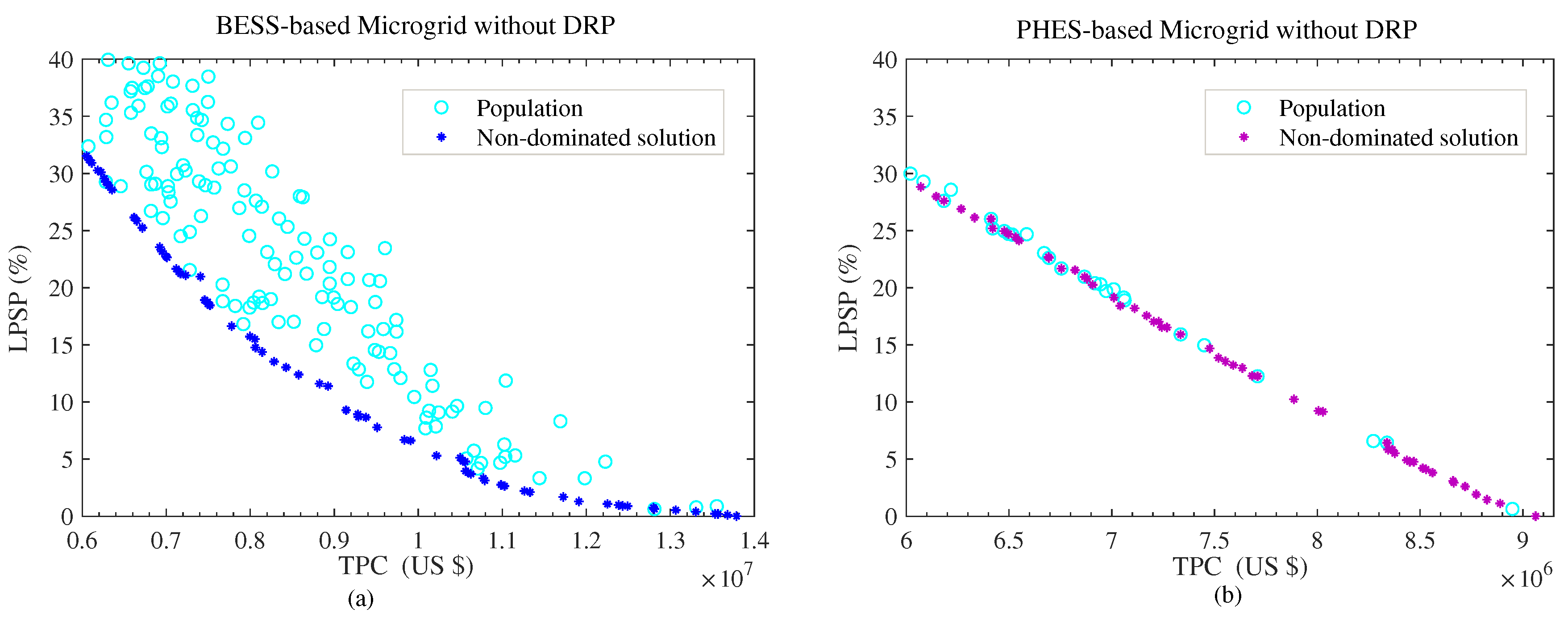
• Case 1: Comparing BESS and PHES without DRP consideration.
• Case 2: Comparing BESS and PHES with CPP DRP consideration.
• Case 3: Comparing BESS and PHES with TADP DRP consideration.

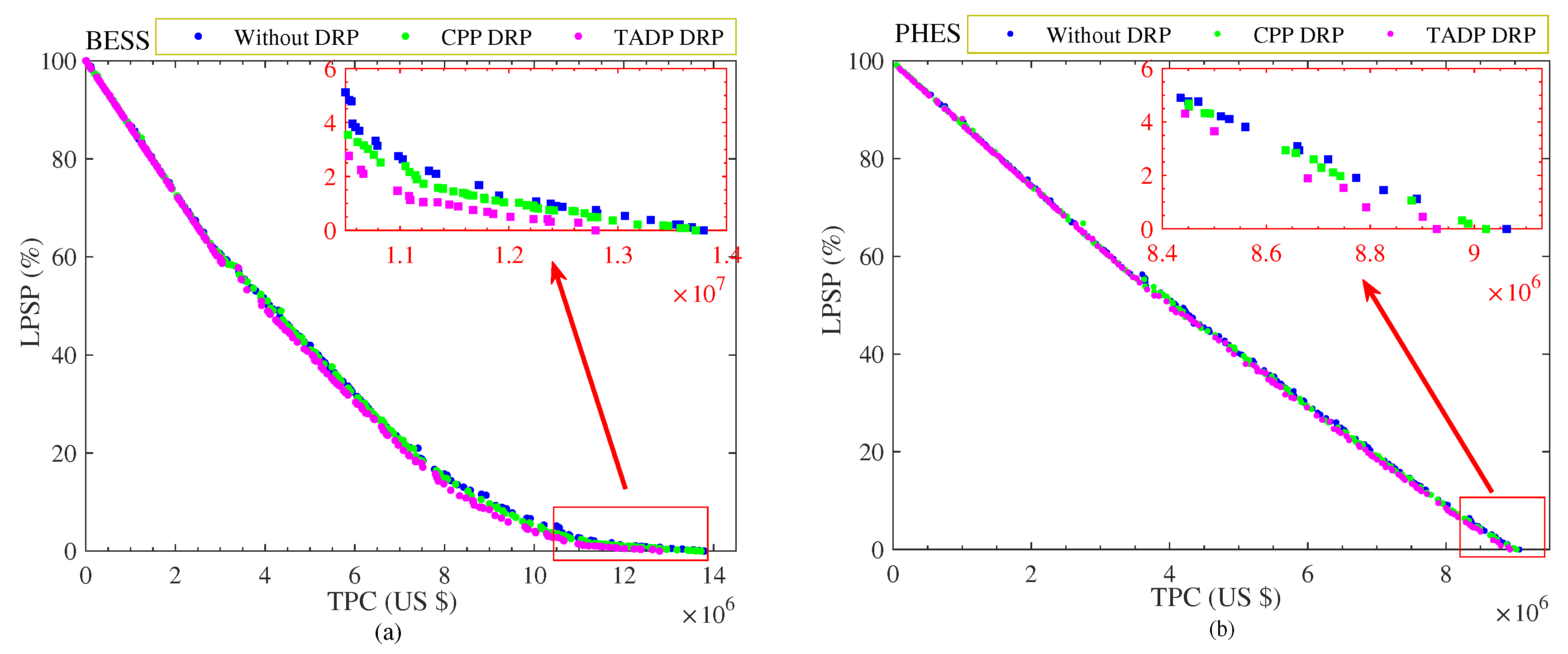
6.1. Case 1: BESS versus PHES without DRP

Figure 4a,b shows the trade-off Pareto front plots for economic and reliability criteria with BESS and PHES, respectively, under case 1. From Figure 4, as expected, the system reliability condition improves (LPSP value decreases) as the total cost increases and vice visa. Hence, the cost-benefit relationship at different LPSP values is analyzed and discussed using the investment cost-savings approach.

Table 3. Techno-economic analysis for case 1.

	BESS-Based Microgrid					PHES-Based Microgrid
LPSP	0%	5%	10%	15%		0%	5%	10%	15%
PV capacity (kW)	1422	1207	1003	1030		1699	1806	1652	1850
WT capacity (kW	1919	2120	2063	1774		1657	1376	1371	1108
ESS capacity (kWh)	6798	1800	900	411		7800	7546	6967	6925
TPC (US $)	1.38 × 10${}^7$	1.05 × 10${}^7$	9.28 × 10${}^6$	8.06 × 10${}^6$		9.06 × 10${}^6$	8.38 × 10${}^6$	8.03 × 10${}^6$	7.59 × 10${}^6$

summarizes the details of the cost-benefit analysis for case 1. The optimal selected points are derived after multiples execution of the optimization program for LPSP values in the range of 0% to 15%.

A comparison of the two systems based on the ESS technology at maximum reliability condition i.e., LPSP = 0%; it can be seen that the choice of PHES instead of BESS results in a total investment cost reduction of about 34.28% from US $ 1.38 × 10${}^7$ to the US $ 9.06 × 10${}^6$. This a significant cost saving in the microgrid planning. Hence, PHES has been shown more economical compared to BESS.

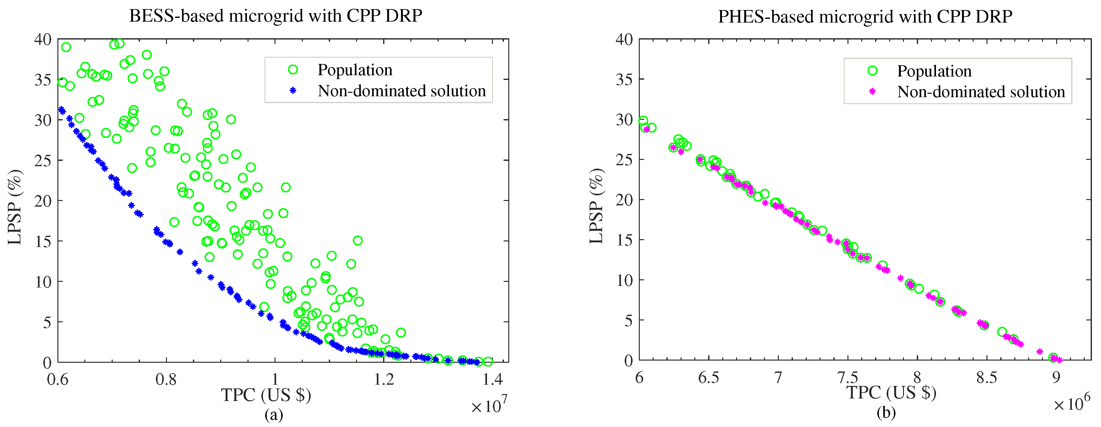
6.2. Case 2: BESS versus PHES with CPP DRP

In this case, the benefit of CPP DRP on capacity sizing optimization problem for both BESS and PHES-based microgrid is investigated, and pareto fronts plotted. Figure 5a,b shows the Pareto front plots with CPP DRP considering BESS and PHES, respectively. For both cases, it can be observed from the pareto plots that an increase in the LPSP value, the TPC decreases, this is due to the fact that the reliability index (LPSP) and planning cost (TPC) are conflicting objective.

Table 4. Techno-economic analysis for case 2.

	BESS-Based Microgrid					PHES-Based Microgrid
LPSP	0%	5%	10%	15%		0%	5%	10%	15%
PV capacity (kW)	1110	1027	958	1039		1826	1670	1754	1671
WT capacity (kW)	2165	2184	2054	1808		1561	1498	1230	1195
ESS capacity (kWh)	6436	1170	670	132		7789	7311	6986	6414
TPC (US $)	1.37 × 10${}^7$	9.91 × 10${}^6$	9.00 × 10${}^6$	7.99 × 10${}^6$		9.02 × 10${}^6$	8.48 × 10${}^6$	7.78 × 10${}^6$	7.49 × 10${}^6$

summarizes the cost–benefits analysis for case 2 which involves the economic effects of critical peak pricing (CPP) DRP for the BESS and PHES-based microgrid configuration.

For the comparative analysis of the two systems configurations at LPSP = 0% (maximum reliability) with the consideration CPP DRP; the selection of PHES as an ESS alternative to BESS in optimum capacity resulted in 34.22% reduction in the total investment costs. This significant cost saving signifies that PHES-based configuration is more economical and preferred investment option compared to BESS-based microgrid.

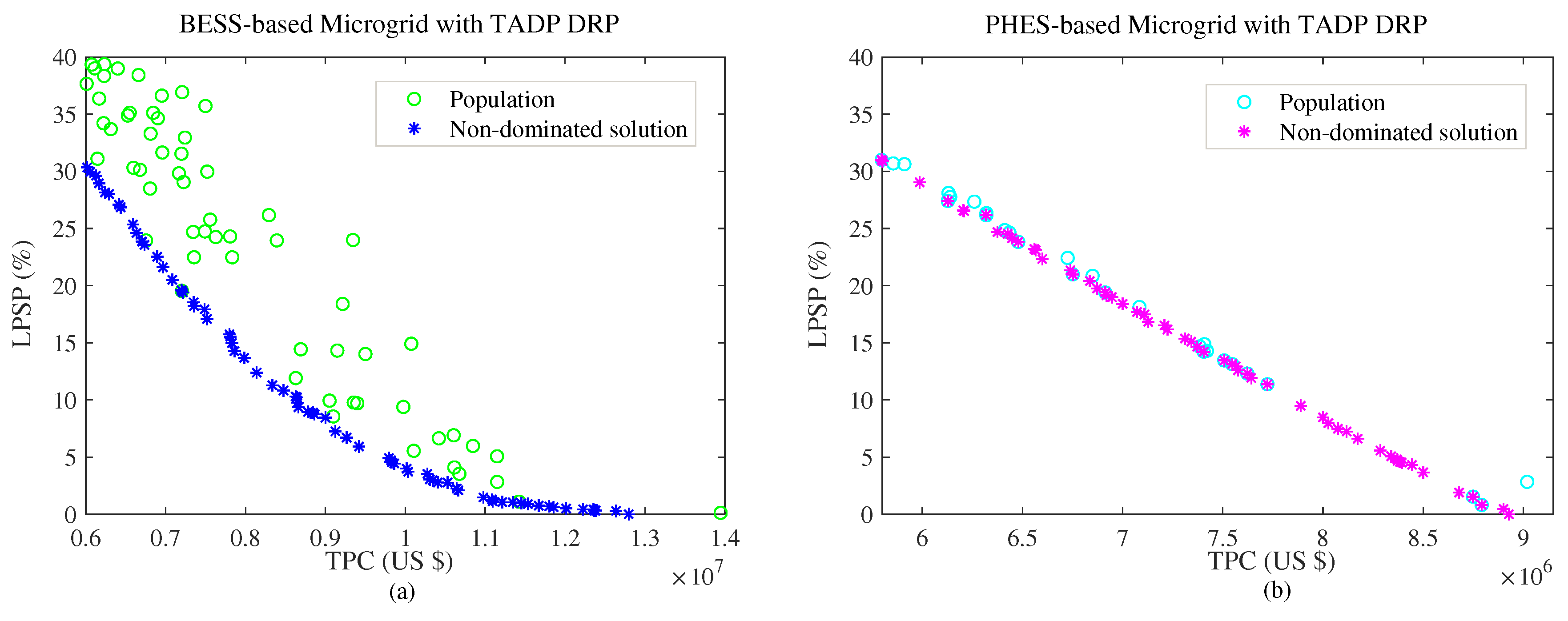
6.3. Case 3: BESS versus PHES with TADP DRP

In this case, the prospects of TADP DRP in optimum component-sizing problem has been investigated. The renewable energy generation forecasting is a subset feature of the TADP DRP implementation. Hence, the GBRT prediction results for wind speed, solar irradiance and the consequent WT and PV powers are validated using error metrics (MAE, RSME and $r^2$) in order to determine the suitable forecasting condition based on the learning rates ${\alpha }_{gbr}$. The total data set contained 17,520 data points with an hourly resolution; from which 75% of the data are adopted for training, and 25% are adopted for testing.

Table 5. Forecasting results of GBRT model based on MAE, RSME and $r^2$ considering three ${\alpha }_{gbr}$ values: ${\alpha }_{gbr}$ = { 0.1, 0.3, 0.5 }.

GBRT Algorithm	Error Metric		${\mathit{\alpha }}_{\mathbf{gbr}}=0.1$	${\mathit{\alpha }}_{\mathbf{gbr}}=0.3$	${\mathit{\alpha }}_{\mathbf{gbr}}=0.5$
Wind speed forecasts	MAE	(m/s)	0.22	0.25	0.28
	RMES	(m/s)	0.27	0.33	0.39
	$r^2$		0.96	0.94	0.92
Wind power forecast	MAE	kW	35.03	39.52	44.33
	RMES	kW	47.98	55.69	62.83
	$r^2$		0.96	0.94	0.92
Solar irradiance forecast	MAE	W/m${}^2$	15.36	18.55	20.35
	RMES	W/m${}^2$	29.62	34.87	40.50
	$r^2$		0.99	0.98	0.98
Photovoltaic power forecast	MAE	kW	17.43	21.05	23.08
	RMES	kW	33.60	39.55	45.94
	$r^2$		0.99	0.98	0.98

summarizes the forecasting results based on MAE, RSME and $r^2$ for the GBRT forecasting model under three ${\alpha }_{gbr}$ values i.e., ${\alpha }_{gbr}$ = 0.1, 0.3, 0.5. As it can be noticed, the chosen value of ${\alpha }_{gbr}$ significantly affects the precision of the GBRT forecasting model.

The best wind speed and wind power forecast results are realized when the ${\alpha }_{gbr}$ value chosen equals 0.1. The least error values indicated by MAE and RMSE of 0.22 (m/s) and 0.27 (m/s) for wind speed prediction and 35.03 kW and 47.98 kW for wind power forecast respectively confirms the consequences of the ${\alpha }_{gbr}$ value chosen. The results accuracy are further validated using the $r^2$ metric; the highest value of $r^2$ = 0.96 further establishes that the GBRT at ${\alpha }_{gbr}$ = 0.1 is an appropriate model for wind speed and wind power forecasting. Figure 6. shows a comparison of the actual wind speed versus the predicted wind speed with one-hour-ahead rolling forecasting horizon using the GBRT model when ${\alpha }_{gbr}$ is set to 0.1 (for the best ${\alpha }_{gbr}$ value).

Also, for solar irradiance and PV power prediction, the best results are obtained when the ${\alpha }_{gbr}$ parameter is set to 0.1. The minimum error values indicated by MAE and RMSE of 15.36 (W/m${}^2$) and 29.62 (W/m${}^2)$ for solar irradiance prediction and 17.43 kW and 33.60 kW for PV power forecast, respectively, validate the parameter selection. Also, the highest $r^2$ metric of 0.99 shows the goodness of fit and suitability of the model selection as being appropriate. Figure 7 shows a comparison of the actual versus the predicted solar irradiances with one-hour-ahead rolling forecasting horizon using the GRBT model when ${\alpha }_{gbr}$ is set to 0.1 (for the best ${\alpha }_{gbr}$ value).

Figure 8a,b shows the Pareto front plots with TADP DRP considering BESS and PHES, respectively; and

Table 6. Techno-economic analysis for case 3.

	BESS-Based Microgrid					PHES-Based Microgrid
LPSP	0%	5%	10%	15%		0%	5%	10%	15%
PV capacity (kW)	1424	1191	1210	1193		1858	1831	1842	1826
WT capacity (kW)	1871	2020	1878	1655		1513	1363	1204	1048
ESS capacity (kWh)	5603	1341	460	181		7494	7326	7121	6397
TPC (US $)	1.28 × 10${}^7$	9.82 × 10${}^6$	8.78 × 10${}^6$	7.83 × 10${}^6$		8.93 × 10${}^6$	8.38 × 10${}^6$	7.89 × 10${}^6$	7.34 × 10${}^6$

summarizes the cost–benefits analysis for the BESS and PHES-based microgrid configuration.

According to the results of optimal capacity sizing considering TADP DRP at LPSP=0%, it can be noted that adoption PHES-based configuration will results in about 30.23% investment costs reduction compared to the BESS-based. Hence, PHES-based microgrid is the most cost-effective microgrid configuration compared to the BESS-based microgrid design. For all the scenarios (case 1–3) investigated, it is seen that PHES gives the lowest investment cost on ESS compared to BESS. Thus, for a cost-effective long-term investment, it can be deduced that the selection of the PHES-based microgrid has a better economic prospect compared to BESS-based configuration.

6.4. Techno-Economic Comparison for Each ESS Type Based on DRP Options at Maximum System Reliability (LPSP = 0%)

In this section, different microgrid configurations based on the DRP options are evaluated based on the net investment cost for different ESS types. The prospect of each configuration in the long-term microgrid planning with the possibility of high renewable energy fraction is reflected in the net investment cost under each system configuration. Figure 9a,b shows the pareto front plots comparison, without and with DRPs, for BESS and PHES-based microgrid design, respectively.

Table 7. Techno-economic analysis for each ESS type based on the DRP flexibility options.

		BESS-Based Microgrid				PHES-Based Microgrid
DRP type		Case 1: without DRP	Case 2: CPP DRP	Case 3: TADP DRP		Case 1: without DRP	Case 2: CPP DRP	Case 3: TADP DRP
PV capacity (kW)		1422	1110	1424		1699	1826	1858
WT capacity (kW)		1919	2165	1871		1657	1561	1513
ESS capacity (kWh)		6798	6436	5603		7800	7789	7494
TPC (US $)		1.38 × 10${}^7$	1.37 × 10${}^7$	1.28 × 10${}^7$		9.06 × 10${}^6$	9.02 × 10${}^6$	8.93 × 10${}^6$
% cost saving		-	0.53%	7.20%		-	0.44%	1.48%

summarizes the investment cost under each configuration and flexibility options. The reference cases are the ones without DRP consideration (case 1) and the cost implication of introducing different types of DRP for each ESS-type microgrid are duly analyzed in terms of percentage cost reduction.

For the BESS-based microgrid, introducing CPP DRP results in a cost saving of 0.53% of the investment from US $ 1.38 × 10${}^7$ (without DRP) to 1.37 × 10${}^7$; this cost saving is as a result of 21.59% and 5.33% reduction in the PV and BESS component sizes, respectively. This is because CPP DRP decreased the load demand and consequentially, the BESS dependency during the peak demand periods. For the PHES-based microgrid, the introduction of CPP DRP results in 0.44% cost reduction from US $ 9.06 × 10${}^6$ to US $ 9.02 × 10${}^6$. The cost-benefit is because of the 5.8% and 0.14% capacity size reduction of WT and PHES, respectively, and an increase of 7.4% PV capacity. For the two cases, It should be noted that there is a decrease in the investment costs as the CPP DRP shifts the FDR to off-peak from the peak period of the system and ensure a more flattened load profile and prevent sub-optimal capacity sizing.

The potential superiority of TADP DRP over CPP DRP for microgrid design for high renewable energy penetration can be seen in the cost–benefits illustrated in Table 7. The inclusion of the TADP DRP in the BESS-based system resulted in 7.2% cost saving in the total planning costs. The planning cost reduction is due to a decrease of 17.58% and 2.5% for BESS and WT respectively with a slight increase of 0.11% in PV component size. Similarly, this trend is noted for PHES-based system with a total cost reduction of 1.48% resulting from 3.98% and 8.69% decrease in PHES and WT capacities, respectively. However, this results in an increase PV capacity of about 9.36%. Figure 10 illustrates the role and impact of DRPs in minimizing the gap between total generated RES power and load demand profiles. The prospects of TADP DRP over CPP DRP to reduce the mismatch between the load and the RES generated power profiles has been vividly portrayed by significant optimum component size reduction and hence the TPC minimization to realize the techno-economic benefit of a microgrid.

Therefore, for the two system and types of DRP investigated, it can be inferred that the application of TADP DRP is more investment-worthy compared to the CPP DRP. TADP DRP short-term flexibility option takes into account the varying generation profile of WT and PV from the forecasting results; thus, the reason for its robustness.

7. Conclusions

This paper investigated the prospects of interlinking the cost of short-term flexibility management of microgrid with the long-term optimal capacity planning models towards achieving a 100% green microgrid by using DRP and forecasting. The long-term capacity planning of energy systems involves the evaluation of the optimal size of each of the system component while the short-term flexibility options are implemented within the optimal energy management strategies. The DRPs are incorporated as flexibility options to minimize the gap between demand and supply, thus minimizing the overall system costs. The forecasting provides an outlook of anticipated generated power proper scheduling for the effective implementation of one of the DRPs employed in this work. The suggested methodology, in this work, seeks to provide a sustainable and cost-effective transformative approach towards achieving a 100% renewable energy generation for Marsabit county microgrid at a reduced cost of investment by cutting down on excessive sizing of system components. This can serve as a benchmark for other under-served isolated regions all over the world.

For the interlinked multi-objective optimization procedure, credible scenarios were investigated considering two ESS technology-based configurations without and with the inclusion of the DRP. DRPs were applied to provide the required operational flexibility that involves shifting the operation of the FDRs from one period to another to minimize the gap between the generation and demand profiles. The two objectives of the techno-economic optimization procedure are the minimization of loss of load probability (LPSP), which is the system reliability criterion and the minimization of the net present value of the investment costs, which is the economic criterion. The forecasting for TADP DRP implementation was performed using the GBRT algorithm on scikit-learn in Python due to its precision and less computational requirement compared to other algorithms, and the MOPSO was adopted for the optimization procedure. The LPSP is set as the standard for economic comparison under each scenario considered in this work. At LPSP = 0%, i.e., maximum system reliability, the potential benefit of TADP DRP outperformed the CPP DRP as reflected on the investment cost component. Also, for the ESS-type performance comparison, PHES was shown to be more cost-effective compared to BESS due to its low cost per kWh of storage capacity and its resultant economic effect on the whole system configuration.

References

1. Senshaw, D.A.; Kim, J.W. Meeting conditional targets in nationally determined contributions of developing countries: Renewable energy targets and required investment of GGGI member and partner countries. Energy Policy 2018, 116, 433–443. [Google Scholar] [CrossRef]
2. Hansen, K.; Mathiesen, B.V.; Skov, I.R. Full energy system transition towards 100% renewable energy in Germany in 2050. Renew. Sustain. Energy Rev. 2019, 102, 1–13. [Google Scholar] [CrossRef]
3. Bramstoft, R.; Skytte, K. Decarbonizing Sweden’s energy and transportation system by 2050. Int. J. Sustain. Energy Plan. Manag. 2017, 14, 3–20. [Google Scholar]
4. Borland, J.; Tanaka, T. Overcoming Barriers to 100% Clean Energy for Hawaii Starts at the Bottom of the Energy Food Chain with Residential Island Nano-Grid and Everyday Lifestyle Behavioral Changes. In Proceedings of the 2018 IEEE 7th World Conference on Photovoltaic Energy Conversion (WCPEC) (A Joint Conference of 45th IEEE PVSC, 28th PVSEC 34th EU PVSEC), Waikoloa, WI, USA, 10–15 June 2018; pp. 3829–3834. [Google Scholar] [CrossRef]
5. Mollenhauer, E.; Christidis, A.; Tsatsaronis, G. Increasing the Flexibility of Combined Heat and Power Plants With Heat Pumps and Thermal Energy Storage. J. Energy Resour. Technol. 2018, 140, 020907. [Google Scholar] [CrossRef]
6. Sakah, M.; Diawuo, F.A.; Katzenbach, R.; Gyamfi, S. Towards a sustainable electrification in Ghana: A review of renewable energy deployment policies. Renew. Sustain. Energy Rev. 2017, 79, 544–557. [Google Scholar] [CrossRef]
7. Khoodaruth, A.; Oree, V.; Elahee, M.; Clark, W.W. Exploring options for a 100% renewable energy system in Mauritius by 2050. Utilities Policy 2017, 44, 38–49. [Google Scholar] [CrossRef]
8. Adewuyi, O.B.; Lotfy, M.E.; Akinloye, B.O.; Howlader, H.O.R.; Senjyu, T.; Narayanan, K. Security-constrained optimal utility-scale solar PV investment planning for weak grids: Short reviews and techno-economic analysis. Appl. Energy 2019, 245, 16–30. [Google Scholar] [CrossRef]
9. Aliyu, A.K.; Modu, B.; Tan, C.W. A review of renewable energy development in Africa: A focus in South Africa, Egypt and Nigeria. Renew. Sustain. Energy Rev. 2018, 81, 2502–2518. [Google Scholar] [CrossRef]
10. Huang, Y.W.; Kittner, N.; Kammen, D.M. ASEAN grid flexibility: Preparedness for grid integration of renewable energy. Energy Policy 2019, 128, 711–726. [Google Scholar] [CrossRef]
11. Papaefthymiou, G.; Dragoon, K. Towards 100% renewable energy systems: Uncapping power system flexibility. Energy Policy 2016, 92, 69–82. [Google Scholar] [CrossRef]
12. Hussain, M.; Gao, Y. A review of demand response in an efficient smart grid environment. Electr. J. 2018, 31, 55–63. [Google Scholar] [CrossRef]
13. Gong, H.; Wang, H. Day-ahead generation scheduling for variable energy resources considering demand response. In Proceedings of the 2016 IEEE PES Asia-Pacific Power and Energy Engineering Conference (APPEEC), Xi’an, China, 25–28 October 2016; pp. 2076–2080. [Google Scholar] [CrossRef]
14. Ding, Y.; Shao, C.; Yan, J.; Song, Y.; Zhang, C.; Guo, C. Economical flexibility options for integrating fluctuating wind energy in power systems: The case of China. Appl. Energy 2018, 228, 426–436. [Google Scholar] [CrossRef]
15. Taibi, E.; Nikolakakis, T.; Gutierrez, L.; Fernandez, C.; Kiviluoma, J.; Rissanen, S.; Lindroos, T.J. Power System Flexibility for the Energy Transition: Part 1, Overview for Policy Makers; International Renewable Energy Agency: Abu Dhabi, UAE, 2018. [Google Scholar]
16. Ma, J.; Silva, V.; Belhomme, R.; Kirschen, D.S.; Ochoa, L.F. Evaluating and planning flexibility in sustainable power systems. In Proceedings of the 2013 IEEE Power & Energy Society General Meeting, Vancouver, BC, Canada, 21–25 July 2013; pp. 1–11. [Google Scholar]
17. Zhou, B.; Xu, D.; Li, C.; Chung, C.Y.; Cao, Y.; Chan, K.W.; Wu, Q. Optimal Scheduling of Biogas–Solar–Wind Renewable Portfolio for Multicarrier Energy Supplies. IEEE Trans. Power Syst. 2018, 33, 6229–6239. [Google Scholar] [CrossRef]
18. Taibi, E.; Nikolakakis, T.; Gutierrez, L.; Fernandez, C.; Kiviluoma, J.; Rissanen, S.; Lindroos, T.J. Power System Flexibility for the Energy Transition: Part 2, IRENA FlexTool Methodology; International Renewable Energy Agency: Abu Dhabi, UAE, 2018. [Google Scholar]
19. Ralon, P.; Taylor, M.; Ilas, A.; Diaz-Bone, H.; Kairies, K. Electricity Storage and Renewables: Costs and Markets to 2030; International Renewable Energy Agency: Abu Dhabi, UAE, 2017. [Google Scholar]
20. Awan, A.B.; Zubair, M.; Sidhu, G.A.S.; Bhatti, A.R.; Abo-Khalil, A.G. Performance analysis of various hybrid renewable energy systems using battery, hydrogen, and pumped hydro-based storage units. Int. J. Energy Res. 2018. [Google Scholar] [CrossRef]
21. Zhang, W.; Maleki, A.; Rosen, M.A.; Liu, J. Optimization with a simulated annealing algorithm of a hybrid system for renewable energy including battery and hydrogen storage. Energy 2018, 163, 191–207. [Google Scholar] [CrossRef]
22. Khiareddine, A.; Salah, C.B.; Rekioua, D.; Mimouni, M.F. Sizing methodology for hybrid photovoltaic /wind/ hydrogen/battery integrated to energy management strategy for pumping system. Energy 2018, 153, 743–762. [Google Scholar] [CrossRef]
23. Huang, Y.; Keatley, P.; Chen, H.; Zhang, X.; Rolfe, A.; Hewitt, N. Techno-economic study of compressed air energy storage systems for the grid integration of wind power. Int. J. Energy Res. 2018, 42, 559–569. [Google Scholar] [CrossRef]
24. Amrollahi, M.H.; Bathaee, S.M.T. Techno-economic optimization of hybrid photovoltaic/wind generation together with energy storage system in a stand-alone micro-grid subjected to demand response. Appl. Energy 2017, 202, 66–77. [Google Scholar] [CrossRef]
25. Jabir, H.; Teh, J.; Ishak, D.; Abunima, H. Impacts of demand-side management on electrical power systems: A review. Energies 2018, 11, 1050. [Google Scholar] [CrossRef]
26. Söder, L.; Lund, P.D.; Koduvere, H.; Bolkesjø, T.F.; Rossebø, G.H.; Rosenlund-Soysal, E.; Skytte, K.; Katz, J.; Blumberga, D. A review of demand side flexibility potential in Northern Europe. Renew. Sustain. Energy Rev. 2018, 91, 654–664. [Google Scholar] [CrossRef]
27. Chen, Y.; Xu, P.; Gu, J.; Schmidt, F.; Li, W. Measures to improve energy demand flexibility in buildings for demand response (DR): A review. Energy Build. 2018, 177, 125–139. [Google Scholar] [CrossRef]
28. Siano, P. Demand response and smart grids—A survey. Renew. Sustain. Energy Rev. 2014, 30, 461–478. [Google Scholar] [CrossRef]
29. Hussain, I.; Mohsin, S.; Basit, A.; Khan, Z.A.; Qasim, U.; Javaid, N. A review on demand response: Pricing, optimization, and appliance scheduling. Procedia Comput. Sci. 2015, 52, 843–850. [Google Scholar] [CrossRef]
30. Neupane, B.; Pedersen, T.B.; Thiesson, B. Utilizing device-level demand forecasting for flexibility markets. In Proceedings of the Ninth International Conference on Future Energy Systems, Karlsruhe, Germany, 12–15 June 2018; ACM: New York, NY, USA, 2018; pp. 108–118. [Google Scholar]
31. González-Aparicio, I.; Zucker, A. Impact of wind power uncertainty forecasting on the market integration of wind energy in Spain. Appl. Energy 2015, 159, 334–349. [Google Scholar] [CrossRef]
32. Martinez-Anido, C.B.; Botor, B.; Florita, A.R.; Draxl, C.; Lu, S.; Hamann, H.F.; Hodge, B.M. The value of day-ahead solar power forecasting improvement. Sol. Energy 2016, 129, 192–203. [Google Scholar] [CrossRef] [Green Version]
33. Notton, G.; Nivet, M.L.; Voyant, C.; Paoli, C.; Darras, C.; Motte, F.; Fouilloy, A. Intermittent and stochastic character of renewable energy sources: Consequences, cost of intermittence and benefit of forecasting. Renew. Sustain. Energy Rev. 2018, 87, 96–105. [Google Scholar] [CrossRef]
34. Gürtler, M.; Paulsen, T. The effect of wind and solar power forecasts on day-ahead and intraday electricity prices in Germany. Energy Econ. 2018, 75, 150–162. [Google Scholar] [CrossRef]
35. Xydas, E.; Qadrdan, M.; Marmaras, C.; Cipcigan, L.; Jenkins, N.; Ameli, H. Probabilistic wind power forecasting and its application in the scheduling of gas-fired generators. Appl. Energy 2017, 192, 382–394. [Google Scholar] [CrossRef] [Green Version]
36. Wang, Q.; Wu, H.; Florita, A.R.; Martinez-Anido, C.B.; Hodge, B.M. The value of improved wind power forecasting: Grid flexibility quantification, ramp capability analysis, and impacts of electricity market operation timescales. Appl. Energy 2016, 184, 696–713. [Google Scholar] [CrossRef] [Green Version]
37. Guangqian, D.; Bekhrad, K.; Azarikhah, P.; Maleki, A. A hybrid algorithm based optimization on modeling of grid independent biodiesel-based hybrid solar/wind systems. Renew. Energy 2018, 122, 551–560. [Google Scholar] [CrossRef]
38. Ramli, M.A.; Bouchekara, H.; Alghamdi, A.S. Optimal sizing of PV/wind/diesel hybrid microgrid system using multi-objective self-adaptive differential evolution algorithm. Renew. Energy 2018, 121, 400–411. [Google Scholar] [CrossRef]
39. Nadjemi, O.; Nacer, T.; Hamidat, A.; Salhi, H. Optimal hybrid PV/wind energy system sizing: Application of cuckoo search algorithm for Algerian dairy farms. Renew. Sustain. Energy Rev. 2017, 70, 1352–1365. [Google Scholar] [CrossRef]
40. Azaza, M.; Wallin, F. Multi objective particle swarm optimization of hybrid micro-grid system: A case study in Sweden. Energy 2017, 123, 108–118. [Google Scholar] [CrossRef]
41. Gazijahani, F.S.; Salehi, J. Reliability constrained two-stage optimization of multiple renewable-based microgrids incorporating critical energy peak pricing demand response program using robust optimization approach. Energy 2018, 161, 999–1015. [Google Scholar] [CrossRef]
42. Kharrich, M.; Akherraz, M.; Sayouti, Y. Optimal sizing and cost of a Microgrid based in PV, WIND and BESS for a School of Engineering. In Proceedings of the 2017 International Conference on Wireless Technologies, Embedded and Intelligent Systems (WITS), Fez, Morocco, 19–20 April 2017; pp. 1–5. [Google Scholar]
43. Balali, M.H.; Nouri, N.; Rashidi, M.; Nasiri, A.; Otieno, W. A multi-predictor model to estimate solar and wind energy generations. Int. J. Energy Res. 2018, 42, 696–706. [Google Scholar] [CrossRef]
44. Howes, J. Concept and development of a pumped heat electricity storage device. Proc. IEEE 2012, 100, 493–503. [Google Scholar] [CrossRef]
45. Desrues, T.; Ruer, J.; Marty, P.; Fourmigué, J. A thermal energy storage process for large scale electric applications. Appl. Therm. Eng. 2010, 30, 425–432. [Google Scholar] [CrossRef] [Green Version]
46. Energy Storage Association. Pumped Heat Electrical Storage (PHES). 2019. Available online: http://energystorage.org/energy-storage/technologies/pumped-heat-electrical-storage-phes (accessed on 15 October 2018).
47. White, A.; Parks, G.; Markides, C.N. Thermodynamic analysis of pumped thermal electricity storage. Appl. Therm. Eng. 2013, 53, 291–298. [Google Scholar] [CrossRef] [Green Version]
48. McTigue, J.D.; White, A.J.; Markides, C.N. Parametric studies and optimisation of pumped thermal electricity storage. Appl. Energy 2015, 137, 800–811. [Google Scholar] [CrossRef] [Green Version]
49. Conteh, A.; Lotfy, M.E.; Kipngetich, K.M.; Senjyu, T.; Mandal, P.; Chakraborty, S. An Economic Analysis of Demand Side Management Considering Interruptible Load and Renewable Energy Integration: A Case Study of Freetown Sierra Leone. Sustainability 2019, 11, 2828. [Google Scholar] [CrossRef]
50. Aalami, H.; Moghaddam, M.P.; Yousefi, G. Evaluation of nonlinear models for time-based rates demand response programs. Int. J. Electr. Power Energy Syst. 2015, 65, 282–290. [Google Scholar] [CrossRef]
51. Javaid, N.; Ahmed, A.; Iqbal, S.; Ashraf, M. Day ahead real time pricing and critical peak pricing based power scheduling for smart homes with different duty cycles. Energies 2018, 11, 1464. [Google Scholar] [CrossRef]
52. Aalami, H.; Moghaddam, M.P.; Yousefi, G. Modeling and prioritizing demand response programs in power markets. Electr. Power Syst. Res. 2010, 80, 426–435. [Google Scholar] [CrossRef]
53. Persson, C.; Bacher, P.; Shiga, T.; Madsen, H. Multi-site solar power forecasting using gradient boosted regression trees. Sol. Energy 2017, 150, 423–436. [Google Scholar] [CrossRef]
54. Coello, C.A.C.; Pulido, G.T.; Lechuga, M.S. Handling multiple objectives with particle swarm optimization. IEEE Trans. Evol. Comput. 2004, 8, 256–279. [Google Scholar] [CrossRef]
55. Weather History Download. Available online: https://www.meteoblue.com (accessed on 11 January 2019).
56. Photovoltaic Geographical Information System. Available online: https://rem.jrc.ec.europa.eu (accessed on 13 January 2019).
57. Power Generation and Transmission Master Plan, Kenya Medium Term Plan 2015–2020—Vol. I; Energy and Petroleum Regulatory Authority: Nairobi, Kenya, 2018.
58. Tarrif Setting: Electricity. Available online: https://www.erc.go.ke/services/economic-regulation (accessed on 14 January 2019).
59. Electricity Cost in Kenya. Available online: https://stima.regulusweb.com/ (accessed on 11 December 2018).
60. Benato, A. Performance and cost evaluation of an innovative Pumped Thermal Electricity Storage power system. Energy 2017, 138, 419–436. [Google Scholar] [CrossRef]
61. Smallbone, A.; Jülch, V.; Wardle, R.; Roskilly, A.P. Levelised Cost of Storage for Pumped Heat Energy Storage in comparison with other energy storage technologies. Energy Convers. Manag. 2017, 152, 221–228. [Google Scholar] [CrossRef]
Figure 1. Proposed system model.
Applsci 09 03855 g001
Figure 2. Schematic diagram of PHES.
Applsci 09 03855 g002
Figure 3. Flowchart for the proposed integrated system planning framework.
Applsci 09 03855 g003
Figure 4. Pareto front plots for case 1.
Applsci 09 03855 g004
Figure 5. Pareto front for case 2.
Applsci 09 03855 g005
Figure 6. Comparison between the actual versus the predicted wind speed with one-hour-ahead rolling forecasting horizon using the GBRT model at α g b r = 0.1 (from 1/12/2018 to 5/12/2018).
Applsci 09 03855 g006
Figure 7. Comparison of the actual versus the predicted solar irradiances with one-hour-ahead rolling forecasting horizon using the GRBT forecasting model at α g b r = 0.1 (from 1/12/2018 to 5/12/2018).
Applsci 09 03855 g007
Figure 8. Pareto front plots for case 3.
Applsci 09 03855 g008
Figure 9. (a,b) shows the Pareto front plots comparison for BESS and PHES-based microgrid design respectively, based on the DRP flexibility options.
Applsci 09 03855 g009
Figure 10. Role and impact of DRPs in minimizing the gap between total generated VRES power and load demand profiles.
Applsci 09 03855 g010