Estimated Impacts of Climate Change on Eddy Meridional Moisture Transport in the Atmosphere

Abstract

Research findings suggest that water (hydrological) cycle of the earth intensifies in response to climate change, since the amount of water that evaporates from the ocean and land to the atmosphere and the total water content in the air will increase with temperature. In addition, climate change affects the large-scale atmospheric circulation by, for example, altering the characteristics of extratropical transient eddies (cyclones), which play a dominant role in the meridional transport of heat, moisture, and momentum from tropical to polar latitudes. Thus, climate change also affects the planetary hydrological cycle by redistributing atmospheric moisture around the globe. Baroclinic instability, a specific type of dynamical instability of the zonal atmospheric flow, is the principal mechanism by which extratropical cyclones form and evolve. It is expected that, due to global warming, the two most fundamental dynamical quantities that control the development of baroclinic instability and the overall global atmospheric dynamics—the parameter of static stability and the meridional temperature gradient (MTG)—will undergo certain changes. As a result, climate change can affect the formation and evolution of transient extratropical eddies and, therefore, macro-exchange of heat and moisture between low and high latitudes and the global water cycle as a whole. In this paper, we explore the effect of changes in the static stability parameter and MTG caused by climate change on the annual-mean eddy meridional moisture flux (AMEMF), using the two classical atmospheric models: the mid-latitude f-plane model and the two-layer β-plane model. These models are represented in two versions: “dry,” which considers the static stability of dry air alone, and “moist,” in which effective static stability is considered as a combination of stability of dry and moist air together. Sensitivity functions were derived for these models that enable estimating the influence of infinitesimal perturbations in the parameter of static stability and MTG on the AMEMF and on large-scale eddy dynamics characterized by the growth rate of unstable baroclinic waves of various wavelengths. For the base climate change scenario, in which the surface temperature increases by 1 °C and warming of the upper troposphere outpaces warming of the lower troposphere by 2 °C (this scenario corresponds to the observed warming trend), the response of the mass-weighted vertically averaged annual mean MTG is $-0.2°\mathrm{C}$ per 1000 km. The dry static stability increases insignificantly relative to the reference climate state, while on the other hand, the effective static stability decreases by more than 5.4%. Assuming that static stability of the atmosphere and the MTG are independent of each other (using One-factor-at-a-time approach), we estimate that the increase in AMEMF caused by change in MTG is about 4%. Change in dry static stability has little effect on AMEMF, while change in effective static stability leads to an increase in AMEMF of about 5%. Thus, neglecting atmospheric moisture in calculations of the atmospheric static stability leads to tangible differences between the results obtained using the dry and moist models. Moist models predict ~9% increase in AMEMF due to global warming. Dry models predict ~4% increase in AMEMF solely because of the change in MTG. For the base climate change scenario, the average temperature of the lower troposphere (up to ~4 km), in which the atmospheric moisture is concentrated, increases by ~$1.5°\mathrm{C}$. This leads to an increase in specific humidity of about 10.5%. Thus, since both AMEMF and atmospheric water vapor content increase due to the influence of climate change, a rather noticeable restructuring of the global water cycle is expected.

1. Introduction

Acceleration in the rate of changes to the earth’s climate system (ECS) that have been observed around the globe and its different geographical regions since the early 20th century has become unprecedented over recent decades [1]. The evidence for rapid and dramatic climate change encompasses increasing the planet’s average surface temperature, rising global sea level, reducing glacier net volumes, decreasing polar ice sheets and sea ice extent, changing heat stores in the ocean, changing rainfall patterns, and a range of other effects. The Fifth Assessment Report of the Intergovernmental Panel on Climate Change (IPCC) states that “Human influence has been detected in warming of the atmosphere and oceans, in changes in the global water cycle, in reductions in snow and ice, in global mean sea level rise, and in changes in some climatic extremes” [1]. One of the clearest indicators of climate change is the rise in global average surface temperature. According to the latest World Meteorological Organization’s (WMO) report “Statement on the State of the Global Climate in 2018” published on March 2019 [2], “The global mean temperature for 2018 is estimated to be 0.99 ± 0.13 °C above the preindustrial baseline (1850–1900).” It is important that over two-third of that global mean temperature increase has occurred after 1980. This WMO’s document also points out that other key climate change indicators (e.g., global mean sea level, Arctic and Antarctic sea-ice extent, greenhouse gas concentrations, extreme natural events) have become even more pronounced. The main cause of the current climate change is human activities and, above all, human-induced substantial emissions of greenhouse gases (GHG) into the atmosphere [1].

Research findings suggest that the shift to a warmer climate is accompanied by intensification of the hydrological (or water) cycle [1,3,4,5,6,7,8,9,10,11] that describes the global circulation of water in its solid, liquid, and gas phases throughout the four geospheres (atmosphere, hydrosphere, lithosphere, and biosphere). The main physical processes that form the planetary hydrological cycle involve evaporation of water (mainly from the ocean surface to the atmosphere), condensation of atmospheric water vapor, multi-scale horizontal moisture transport (advection), precipitation that can take on different forms (e.g., rain, snow, ice crystals), runoff and snowmelt, interception, infiltration, transpiration, percolation, and storage. The hydrological cycle intensifies under global warming mainly because the amount of water that evaporates from the ocean and land to the air and the total water vapor content in the atmosphere will increase with temperature. Theoretical estimates and satellite observations suggest that as air temperature increases the saturated water vapor pressure increases as well by about 7% per Kelvin [5,12,13]. Indeed, let us write the approximate Clausius-Clapeyron relation assuming the latent heat of vaporization $L_w$ is a constant:

$$\frac{d\ln e_s}{dT}=\frac{L_v}{R_v{T}^2}.$$

According to this equation, an infinitesimal change in temperature $\Delta T$ is accompanied by a fractional change $\Delta e_s/e_s$ in saturation vapor pressure of:

$$\frac{\Delta e_s}{e_s}\approx \frac{L_v}{R_v{T}^2}\Delta T.$$

Taking the value of $T_0=273.16\mathrm{K}$ as a reference temperature, we obtain that the fractional growth in $e_s$ is ~7% K⁻¹, meaning that to increase the temperature by 1 K results in the 7% increase in saturation vapor pressure. The observations also indicate that over the last two to three decades the precipitation has increased at about the same rate [12]. Since the hydrological cycle has a significant impact on the climate of our planet, its strengthening with rising global temperature may alter the weather patterns worldwide. Changes in frequency and intensity of extreme weather events (e.g., storms), precipitation, heavy rainfall, and flooding are the potential impacts of an intensified water cycle. However, the potential future alterations in the earth’s climate and weather conditions in response to the human-induced planet’s warming will not be geographically homogeneous [1]. Some parts of the world will experience more pronounced changes, but some regions will experience less noticeable changes. In particular, main characteristics of rainfall and other forms of precipitation (their amount, intensity and frequency) will experience strong spatial variations [14]. Greater volume of precipitation is expected in high latitude regions and in the tropics, while in subtropical arid and semi-arid regions and many mid-latitude regions rainfall amounts will decrease [1,15,16,17,18]. Consequently, geographical areas with increased amount, intensity and frequency of precipitation and, moreover, areas that will also be seriously affected by sea level rise (coastal areas), will likely to experience increased risk of hazardous hydrological events, such as flooding.

The spatial and temporal heterogeneity of climate change (variations in the trend (cooling or warming) and magnitude of climate change over space) is determined not only by the geographic location of the region in question, but also by the general circulation of the atmosphere (GCA) which involves a wealth of air motions with scales on the order of thousands of kilometers such as the westerly mean flow in the mid-latitudes in both the northern and southern hemispheres, planetary waves, large-scale extratropical transient eddies (cyclones and anticyclones), monsoons, and trade winds [19,20,21,22,23,24]. One of the main dynamical mechanisms leading to the meridional transport of heat, moisture, and momentum from the tropical to polar latitudes and, thereby to the global redistribution of atmospheric moisture, are the large-scale extratropical eddies (cyclones) [19,20,21,22]. The so-called “atmospheric rivers” that transport water vapor outside of the tropics through the extratropics (middle latitudes) are associated with mid-latitude cyclonic eddies and their frontal zones [25,26]. Recent studies have indicated an increase in intensity of extratropical cyclones and a decrease in their frequency [27,28,29,30,31,32,33,34]. Baroclinic instability, a specific type of dynamical instability of the zonal atmospheric flow with the equator-to-pole (meridional) temperature contrast (gradient) and, therefore, with a vertical wind shear (thermal wind), in the field of Coriolis force, is the principal mechanism by which extratropical cyclones form and evolve [35,36,37,38]. The infinitesimal perturbations growing in such a flow derive their energy from the transformation of mean available potential energy (MAPE) which, in turn, depends on the tropospheric meridional temperature gradient (MTG); the larger the temperature differences between the equator and the pole, the greater the MAPE [39,40,41]. However, MTG is not the only fundamental parameter that determines the development of baroclinic instability in the atmosphere and, therefore, the formation of extratropical large-scale cyclonic eddies. The effective static stability of the atmosphere plays an equally important role in the generation of cyclones (e.g., [42,43,44,45]). Unlike the so-called “dry static stability” of the atmosphere [21], the effective static stability takes into consideration not only the vertical thermal stratification of the air (temperature lapse rate $\mathsf{\Gamma }=-\partial T/\partial z$, where T is an air temperature, and z is a vertical coordinate), but also the effects of water vapor condensation, namely latent heat released into the atmosphere when the water vapor changes its state to a liquid. In consequence of latent heating, the effective stability of the moist atmosphere in mid-latitudes is less than the static stability of the dry atmosphere by about 40% [45]. It should be emphasized that the latent heat energy also affects the formation and development of extratropical cyclones contributing to their intensification (e.g., [46,47,48,49,50]).

Results of climate simulations and observational data indicate changes in atmospheric thermodynamics and large-scale circulations that have become especially apparent in recent decades (e.g., [51,52,53,54,55,56]). However, human-induced tropospheric warming is not uniform across the globe [1]. The most prominent warming is observed in the northern polar region near the surface (polar amplification phenomenon [57,58]) and at the upper equatorial troposphere implying changes in both static stability and MTG [59]. As a result of this warming, static stability increases in mid-latitude and tropical areas and decreases in polar areas [59,60,61,62]. In turn, the MTG increases in the higher altitudes and decreases at the surface which can provide, respectively, favorable and adverse conditions for the formation of large-scale extratropical eddies [52,56,59,63,64]. Thus, with global warming, static stability and MTG are expected to undergo certain changes affecting the formation and evolution of transient extratropical eddies, which will impact the heat and moisture macro-exchange between low and high latitudes, and, thereof, the earth’s hydrological cycle.

In this paper, we explore the effect of changes in the static stability parameter and MTG caused by climate change on the annual-mean eddy meridional moisture flux (AMEMF), using the two classical atmospheric models: the mid-latitude f-plane model [36] and the two-layer β-plane model [37]. These models are represented in two versions: “dry,” which considers the static stability of dry air alone, and “moist,” in which effective static stability is considered as a combination of stability of dry and moist air together. Sensitivity functions were derived for these models that enable estimating the influence of infinitesimal perturbations in the parameter of static stability and MTG on the AMEMF and on large-scale eddy dynamics characterized by the growth rate of unstable baroclinic waves of various wavelength.

2. Materials and Methods

2.1. Moisture Content and Transport in the Global Atmosphere

Earth’s climate system is made up of five basic parts: the atmosphere, hydrosphere, cryosphere, lithosphere, and biosphere, which interact with each other evolving over time and responding to internal and external perturbations. All the water on the earth form the hydrosphere which is commonly called “the water shell of our planet.” Estimates indicate that the aggregated volume of water on earth is around 1.38 × 10⁹ km³ [65,66]. The prevailing portion of this, ~1.34 × 10⁹ km³ (about 97% of the total volume), is in the oceans. Oceans form the largest water reservoir on earth. The second largest global water reservoir includes ice sheets, sea ice, and glaciers containing a total of about 23 × 10⁶ km³ (~1.7% of total planetary volume of water) followed by groundwater (~18 × 10⁶ km³ of water or ~1.3% of the total volume). Apart from that, much smaller volumes of water are contained in lakes, rivers, and streams (~18 × 10⁴ km³ of water or ~0.013% of the total volume) and in the atmosphere (~13 × 10³ km³ of water or ~0.00094% of the total volume) [65,66].

In the atmosphere, the volumetric water vapor content varies almost from zero to 4%, and considerably changes across the globe and is subject to seasonal influence. The content of water vapor reaches its maximum at the earth’s surface and decreases rapidly with height. For example, at an altitude of 5 km, the water vapor content is nearly ten times less than that of the earth’s surface, and at an altitude of 8 km—one hundred times less. Thus, above 10–15 km, the content of water vapor in the air is negligible [67]. Despite the fact that the amount of water contained in the atmosphere is much less than the total available water on earth, it would be very difficult to overestimate the key role of atmospheric water vapor in forming the energy balance of our planet and global hydrological cycle [68,69,70].

Water vapor along with carbon dioxide, methane, and ozone, forms the group of the major atmospheric GHGs [1]. Most likely that if there were no GHGs in the earth atmosphere, then our planet would hardly have been inhabited by humans. In fact, the water vapor is the most crucial natural GHG that is responsible for more than 60% of the total earth’s greenhouse effect [71]. The positive feedback of water vapor in climate system is well-known; an increase in the atmospheric temperature caused by other factors increases water evaporations from oceans, lakes, rivers, and soil leading to rising concentrations of water vapor in the atmosphere and consequently increasing the greenhouse effect [1]. On the other hand, growing moisture content in the atmosphere contributes to the formation of cloud cover, which, in turn, reflects shortwave solar radiation, thereby increasing the planetary albedo. This leads to an anti-greenhouse effect [72]. Thus, the effect of atmospheric moisture on climate processes is complex and of varied nature.

In analyzing the global distribution and transport of moisture in the atmosphere, the balance equation can be written as [73]:

$$\frac{\partial W}{\partial t}+\nabla \cdot Q=E-P$$

(1)

Here W is the amount of precipitable water within the atmospheric column extending above the earth’s surface of unit area, Q is the vertically integrated horizontal moisture flux, E is the rate of evaporation, and P is the rate of precipitation from the atmospheric column. Note that

$$W=\frac{1}{g}{\displaystyle {\int }_0^{p_0}qdp}$$

(2)

$$Q={\displaystyle {\int }_0^{p_0}qV\frac{dp}{g}}=\underset{\mathrm{Zonal}\mathrm{component}{Q}_{\lambda }}{\underbrace{i_{\lambda }{\displaystyle {\int }_0^{p_0}qu\frac{dp}{g}}}}+\underset{\mathrm{Meridional}\mathrm{component}{Q}_{\phi }}{\underbrace{i_{\phi }{\displaystyle {\int }_0^{p_0}qv\frac{dp}{g}}}}$$

(3)

In this study, the quantity of interest is the mean vertically integrated meridional moisture flux (MMF) ${\overline{Q}}_{\phi }$, which can be decomposed into three components [73]:

$$\underset{\mathrm{MMF}}{\underbrace{\left\{\left[\overline{\mathrm{qv}}\right]\right\}}}=\underset{\mathrm{MMC}}{\underbrace{\left\{\left[\overline{q}\right]\left[\overline{v}\right]\right\}}}+\underset{\mathrm{SE}}{\underbrace{\left\{\left[{\overline{q}}^{\ast }{\overline{v}}^{\ast }\right]\right\}}}+\underset{\mathrm{TE}}{\underbrace{\left\{\left[\overline{q^{\prime }{v}^{\prime }}\right]\right\}}}$$

(4)

The first term on the right-hand side of this equation (MMC) is the contribution from mean meridional circulation, the second term (SE) is from stationary eddies (planetary waves), and the third term (TE) is from transient eddies (extratropical cyclones) [67,68]. Numerous studies involving the evaluation of the right-hand side of Equation (4) with observations datasets and CGCM-simulated data (Coupled atmosphere-ocean general circulation model) have shown that transient eddies dominate meridional moisture transport at mid-latitudes: ~80% between 30° and 40° north and south latitudes (e.g., [20,40,41,68,73,74,75,76,77]). One can easily show that for the plane wave solutions (A15), the TE meridional moisture flux is exponentially dependent on the growth rate ${\chi }_k=k{c}_i$ of unstable modes [78]. Let $L_w$ be the wavelength of a baroclinic unstable wave and $k=2\mathsf{\pi }/L_w$ its wavenumber. Then

$$q^{\prime }\left(x,p,t\right)=\Re e\left(\widehat{q}\left(p\right)e^{ik\left(x-ct\right)}\right),v^{\prime }\left(x,p,t\right)=\Re e\left(\widehat{v}\left(p\right)e^{ik\left(x-ct\right)}\right)$$

(5)

or

$$q^{\prime }\left(x,p,t\right)=\left|\widehat{q}\left(p\right)\right|\cos \left[k\left(x-c_{r}t\right)+{\theta }_q\left(p\right)\right]e^{k{c}_{i}t}$$

(6)

$$v^{\prime }\left(x,p,t\right)=\left|\widehat{v}\left(p\right)\right|\cos \left[k\left(x-c_{r}t\right)+{\theta }_v\left(p\right)\right]e^{k{c}_{i}t}$$

(7)

where $\left|\widehat{q}\left(p\right)\right|$ and $\left|\widehat{v}\left(p\right)\right|$ are the absolute values and ${\theta }_q\left(p\right)$ and ${\theta }_v\left(p\right)$ are the arguments of the complex values $\widehat{q}\left(p\right)$ and $\widehat{v}\left(p\right)$ respectively, $c_r=\Re e\left(c\right),c_i=\Im m\left(c\right)$.

The meridional equator-to-pole moisture flux averaged over one period of the unstable wave with wavelength $L_w$ is as follows [21]:

$${\overline{q^{\prime }{v}^{\prime }}}^x=\frac{1}{L_w}{{\displaystyle \int }}_0^{L_w}{q}^{\prime }\left(x,p,t\right)v^{\prime }\left(x,p,t\right)dx$$

(8)

We can find the flux ${\overline{q^{\prime }{v}^{\prime }}}^x$ by substituting (6) and (7) into (8) and assuming the periodic boundary conditions along the x axis:

$$\begin{array}{c}{\overline{q^{\prime }{v}^{\prime }}}^x=\frac{k}{2\mathsf{\pi }}{\mathrm{e}}^{2k{c}_{i}t}{{\displaystyle \int }}_0^{2\mathsf{\pi }/k}\left|\widehat{q}\left(p\right)\right|\cos \left[k\left(x-c_{r}t\right)+{\theta }_q\left(p\right)\right]\left|\widehat{v}\left(p\right)\right|\cos \left[k\left(x-c_{r}t\right)+{\theta }_u\left(p\right)\right]dx\\ =\frac{k}{2\mathsf{\pi }}{\mathrm{e}}^{2k{c}_{i}t}{{\displaystyle \int }}_0^{2\mathsf{\pi }/k}\left|\widehat{q}\left(p\right)\right|\left|\widehat{v}\left(p\right)\right|\cos \left[{\theta }_q\left(p\right)-{\theta }_u\left(p\right)\right]dx\\ \underset{=0}{\underbrace{+\frac{k}{2\mathsf{\pi }}{\mathrm{e}}^{2k{c}_{i}t}{{\displaystyle \int }}_0^{2\mathsf{\pi }/k}\left|\widehat{q}\left(p\right)\right|\left|\widehat{v}\left(p\right)\right|\cos \left[2k\left(x-c_{r}t\right)+{\theta }_q\left(p\right)+{\theta }_u\left(p\right)\right]dx}}\\ =\frac{1}{2}\left|\widehat{q}\left(p\right)\right|\left|\widehat{v}\left(p\right)\right|\cos \left[{\theta }_q\left(p\right)-{\theta }_u\left(p\right)\right]{\mathrm{e}}^{2k{c}_{i}t}\\ =\frac{1}{2}\Re e\left(\widehat{q}\left(p\right){\widehat{v}}^{*}\left(p\right)\right){\mathrm{e}}^{2k{c}_{i}t}\end{array}$$

(9)

The product $k{c}_i={\chi }_k$ with dimension ${\mathrm{day}}^{-1}$ is referred to as the growth rate of a baroclinic unstable wave with wavenumber of k. From the above equation, it follows that the growth rate ${\chi }_k$ significantly affects the meridional eddy moisture transport in the atmosphere. Global warming enhances this effect since, as mentioned in the introduction, an increase in temperature leads to an increase in water vapor content in the atmosphere. We should note that the growth rate ${\chi }_k$ depends upon the two variables, wavenumber k (or wavelength $L_w$) of the unstable wave, and imaginary part of the phase speed $c_i$. Thus, the influence of changes in both $L_w$ and $c_i$ on ${\chi }_k$ will be explored below.

2.2. Sensitivity Functions for Estimating the Influence of Global Warming on the Grouth Rate of Unstable Waves

To estimate the influence of global warming on the growth rate of unstable baroclinic waves, let us consider the expression for ${\chi }_k$ valid for the f-plane model (see Equation (A23) in the Appendix A.2):

$${\chi }_k=\frac{\mathsf{\Lambda }{f}_0}{2\sqrt{{\sigma }_0}}\sqrt{\left|{\eta }^2-4\left(\eta \coth \eta -1\right)\right|}$$

(10)

where $\eta =p_{0}k\sqrt{{\sigma }_0}/f_0$.

This equation shows that at a given latitude, the growth rate ${\chi }_k$ is dependent on a vertical wind shear $\mathsf{\Lambda }$, static stability ${\sigma }_0$, and quantity η which, in turn, depends on the static stability ${\sigma }_0$ and horizontal wavenumber k. As we discussed above, with global warming both the atmospheric static stability and the vertical wind shear, via MTG, are changed and by this way influence the development of baroclinic instability. Thus, the impact of climate change on ${\chi }_k$ can be estimated via variations in ${\sigma }_0$ and $\mathsf{\Lambda }$ around their certain reference values ${\sigma }_0^{ref}$ and ${\mathsf{\Lambda }}^{ref}$, which correspond to the current climate conditions [79]. Let $\delta {\sigma }_0$ and $\delta \mathsf{\Lambda }$ be infinitesimal perturbations in the parameters ${\sigma }_0$ and $\mathsf{\Lambda }$ caused by climate change. Note that $\delta {\sigma }_0\ll {\sigma }_0^{ref}$ and $\delta \mathsf{\Lambda }\ll {\mathsf{\Lambda }}^{ref}$. To quantify the effect of small perturbations $\delta {\sigma }_0$ and $\delta \mathsf{\Lambda }$ on the growth rate ${\chi }_k$, we shall use the sensitivity functions $S_{\sigma }$ and $S_{\mathsf{\Lambda }}$ defined as the partial derivatives of ${\chi }_k$ with respect to parameters ${\sigma }_0$ and $\mathsf{\Lambda }$, respectively, calculated around the reference values ${\sigma }_0^{ref}$ and ${\mathsf{\Lambda }}^{ref}$. Then, the variation in the growth rate of unstable modes $\delta {\chi }_k$ due to variations in the parameters ${\sigma }_0$ and $\mathsf{\Lambda }$ is estimated as follows:

$$\delta {\chi }_k\approx \delta {\sigma }_0\times {S_{\sigma }|}_{{\sigma }_{0=}{\sigma }_0^{ref}}$$

(11)

$$\delta {\chi }_k\approx \delta \mathsf{\Lambda }\times {S_{\mathsf{\Lambda }}|}_{\mathsf{\Lambda }={\mathsf{\Lambda }}^{ref}}$$

(12)

where sensitivity functions are defined by

$$S_{\sigma }=\frac{{\chi }_k}{2{\sigma }_0}\left[p_0\sqrt{{\sigma }_0}\frac{k}{f_0}\frac{\eta -2\coth \eta +2\eta {\mathrm{csch}}^2\eta }{{\eta }^2-4\left(\eta \coth \eta -1\right)}-1\right]$$

(13)

$$S_{\mathsf{\Lambda }}=\frac{f_0}{2\sqrt{{\sigma }_0}}\sqrt{\left|{\eta }^2-4\left(\eta \coth \eta -1\right)\right|}$$

(14)

Considering baroclinic instability on the β-plane [37] whereby the Coriolis parameter, f, is set to vary linearly in the y-direction, we derived the following expression for the growth rate of unstable waves (see Equation (A35) in the Appendix A.3):

$${\chi }_k=\frac{\sqrt{\left|{\beta }^2{\mu }^4+u_T^2{k}^4\left(k^4-4{\mu }^4\right)\right|}}{k\left(k^2+2{\mu }^2\right)}$$

(15)

Here ${\mu }^2=f_0^2/\left[{\sigma }_0{\left(\Delta p\right)}^2\right]$ and $u_T=\left(u_1-u_2\right)/2$, where $u_1$ and $u_2$ are the wind speeds at 250 hPa and 750 hPa pressure levels respectively.

Differentiating the above equation with respect to parameters, ${\sigma }_0$ and $u_T$, we find the sensitivity functions which characterize the influence of static stability and MTG on the growth rate of baroclinic unstable waves:

$$S_{\sigma }=-\frac{k{\mu }^2}{{\sigma }_0{\left(k^2+2{\mu }^2\right)}^2}\frac{2u_T^2{k}^4\left(k^4+2{\mu }^2\right)-{\beta }^2{\mu }^2}{u_T^2{k}^4\left(k^4-4{\mu }^4\right)+{\beta }^2{\mu }^4}\sqrt{u_T^2{k}^4\left(k^4-4{\mu }^4\right)+{\beta }^2{\mu }^4}$$

(16)

$$S_{u_T}=-u_T{k}^3\left(k^2-2{\mu }^2\right)\frac{\sqrt{\left|{\beta }^2{\mu }^4+u_T^2{k}^4\left(k^4-4{\mu }^4\right)\right|}}{{\beta }^2{\mu }^4+u_T^2{k}^4\left(k^4-4{\mu }^4\right)}$$

(17)

The variation in the growth rate of unstable modes $\delta {\chi }_k$ due to variations in the parameter $u_T$ is estimated by the following sensitivity function:

$$\delta {\chi }_k\approx \delta u_T\times {S_{u_T}|}_{u_T=u_T^{ref}}$$

(18)

In addition to the absolute sensitivity functions, $S_{\alpha }$ ($\alpha =\sigma ,\mathsf{\Lambda },u_T$), relative sensitivity functions, $S_{\alpha }^R$, are used to estimate the relative influence of the model parameters on the growth rate of unstable waves, which allow ranking the parameters by the degree of influence of their variations on the variations on the growth rate. Relative sensitivity function is defined by [80]

$$S_{\alpha }^R={\frac{{\alpha }_0}{{\chi }_k}\frac{\partial {\chi }_k}{\partial \alpha }|}_{\alpha ={\alpha }_0}=\frac{{\alpha }_0}{{\chi }_k}{S}_{\alpha }$$

(19)

where ${\alpha }_0$ is a certain reference value of the parameter $\alpha$.

3. Results

3.1. Qualitative Analysis

Extratropical transient cyclonic eddies are wave phenomena, which are formed and evolved in response of the baroclinic instability of atmospheric quasi-zonal westerly flows drawing energy from the MAPE that arises from the MTG. As shown in the previous section, the meridional moisture flux depends on the wavelength of unstable wave which characterizes the size of cyclones. Numerous studies (e.g., [27,28,29,30,31,32,33,34,81,82]) suggest that over the past few decades the length-scale, frequency, and intensity of extratropical cyclones have changed, and a poleward shift of storm tracks and eddy driven jet streams have been observed. Apart from that, the projected changes in the climate system will, to a certain extent, affect the genesis and development of large-scale eddies in the mid-latitude atmosphere [83]. The impact of global warming on the horizontal sizes of transient eddies and their activity (the number of cyclones generated annually) can be qualitatively examined using a simplified theoretical framework (e.g., [84]). In a baroclinic atmosphere, the characteristic horizontal length scale of eddies is determined by the first internal Rossby radius of deformation $L_R$ [21]:

$$L_R=\frac{NH}{f}=\frac{1}{f}\sqrt{\frac{T}{g}\left({\mathsf{\Gamma }}_d-\mathsf{\Gamma }\right)}$$

(20)

where H is the height of homogeneous atmosphere. In the mid-latitudes, typical values for H, N, and f are respectively 8 km, 10⁻² s⁻¹, and 1.1 × 10⁻⁴ s⁻¹ [21], consequently $L_R\approx 850$ km.

The impact of global warming on $L_R$ can be estimated by the sensitivity coefficient $d{L}_R/dT$. Using logarithmic differentiation to differentiate both sides of Equation (20) with respect to T, we obtain

$$\frac{1}{L_R}\frac{d{L}_R}{dT}=\frac{1}{2}\left[\frac{1}{T}-\frac{d\Gamma }{dT}{\left({\Gamma }_d-\Gamma \right)}^{-1}\right]$$

(21)

Equation (21) shows that in baroclinic atmosphere the influence of temperature growth on $L_R$ is not so clear. The dry adiabatic lapse rate ${\mathsf{\Gamma }}_d$ is a constant $9.8°\mathrm{C}$ km⁻¹, while the typical value for $\mathsf{\Gamma }$ is about $6.5°\mathrm{C}$ km⁻¹. Since ${\mathsf{\Gamma }}_d>\mathsf{\Gamma }$ and 1/T are small, depending on the behavior of $\mathsf{\Gamma }$ under global warming, there could be two possible contrasting scenarios, $d{L}_R/dT>0$ and $d{L}_R/dT<0$. Therefore, in order to get a more clear picture of the global warming impact on $L_R$, it is useful to explore these two scenarios. To begin, let us consider partial sensitivity coefficients:

$$\frac{1}{L_R}\frac{\partial L_R}{\partial T}=\frac{1}{2T}$$

(22)

$$\frac{1}{L_R}\frac{\partial L_R}{\partial \mathsf{\Gamma }}=-\frac{1}{2\left({\mathsf{\Gamma }}_d-\mathsf{\Gamma }\right)}$$

(23)

From Equation (22), it follows that a small change $\Delta T$ in temperature causes a fractional change $\Delta L_R/L_R$ in Rossby radius of deformation of

$$\frac{\Delta L_R}{L_R}\approx \frac{1}{2T}\Delta T$$

(24)

Taking the annual global mean surface temperature $T_{sfc}\approx 288\mathrm{K}$ as a reference temperature, we find that $\left(1/L_R\right)\left(\partial L_R/\partial T\right)$ is about $0.002{\mathrm{K}}^{-1}$ which means that to increase the temperature by 1 K leads only to the 0.2% increase in characteristic length of large-scale eddies. Similarly, we can estimate the effect of small changes in the temperature lapse rate $\Delta \mathsf{\Gamma }$ on a fractional change $\Delta L_R/L_R$:

$$\frac{\Delta L_R}{L_R}\approx -\frac{1}{2\left({\mathsf{\Gamma }}_d-\mathsf{\Gamma }\right)}\Delta \mathsf{\Gamma }$$

(25)

The characteristic value of $\mathsf{\Gamma }$ in the mid-latitude troposphere is 6.5 K/km, hence the partial sensitivity $\left(1/L_R\right)\left(\partial L_R/\partial \mathsf{\Gamma }\right)$ is about $-0.15{\mathrm{kmK}}^{-1}$, meaning that to increase the lapse rate by 1 K/km (i.e., reducing the atmospheric static stability) results in the 15% decrease in characteristic length of large-scale eddies.

Estimating the total sensitivity coefficient $\left(1/L_R\right)\left(d{L}_R/dT\right)$ using Equation (20) is not a trivial task since this requires a priori knowledge of interdependence between the temperature increase and the lapse rate change. It should be added that to take into consideration the effects of atmospheric moisture on sensitivity coefficients (21) and (23), instead of dry adiabatic lapse rate ${\mathsf{\Gamma }}_d$ we would have to use the “effective” lapse rate defined by ${\mathsf{\Gamma }}_e={\mathsf{\Gamma }}_d-\left({\mathsf{\Gamma }}_d-{\mathsf{\Gamma }}_m\right){\delta }_{cloud}$, where ${\mathsf{\Gamma }}_m$ is the moist adiabatic lapse rate and ${\delta }_{cloud}$ is a cloud fraction. However, the sensitivity coefficient (21) can be estimated by using observations and/or results of climate modeling. For example, for mid-latitudes, the estimates of the total and partial sensitivity coefficients (21)–(23) were obtained in [84] from NCEP/NCAR reanalysis data and from climate modeling. The estimate of $\left(1/L_R\right)\left(d{L}_R/dT\right)$ is about $-0.0016\left(\pm 0.0096\right)$ K⁻¹ from the reanalysis data, and $-0.0013$ K⁻¹ and $-0.021$ K⁻¹ from the results of simulations for dry and moist atmosphere respectively. The estimate of partial sensitivity coefficient $\left(1/L_R\right)\left(\partial L_R/\partial T\right)$ is about 0.009 (±0.007) K⁻¹ from the reanalysis data and 0.002 K⁻¹ from the modeling results. In turn, the estimate of partial sensitivity coefficient $\left(1/L_R\right)\left(\partial L_R/\partial \mathsf{\Gamma }\right)$ is $-0.309\left(\pm 0.062\right)$ km K⁻¹ from the reanalysis data, and $-0.132$ kmK⁻¹ and $-0.270$ kmK⁻¹ from the outcomes of simulations for dry and moist atmosphere respectively. Thus, the atmospheric vertical stratification (the lapse rate $\mathsf{\Gamma }$), which changes with global warming, and atmospheric moisture can affect the horizontal length of baroclinic extratropical transient eddies, leading in aggregate to a decrease in $L_R$. However, this decrease is insignificant. For example, results of numerical modeling show that the climate change leads only to the 2% decrease in characteristic length of large-scale eddies [84,85]. We should note that it is not possible to compare sensitivity functions $\left(1/L_R\right)\left(\partial L_R/\partial T\right)$ and $\left(1/L_R\right)\left(\partial L_R/\partial \mathsf{\Gamma }\right)$ as they are sensitivities with respect to different quantities and thus have different dimensions and equivalence classes.

For reference purpose, we also consider the influence of global warming on cyclones’ frequency of occurrence using the sensitivity coefficient $\left(1/n\right)\left(dn/dT\right)$, where n is the annual mean number of extratropical cyclones in the northern (or southern) hemisphere [86]:

$$\frac{1}{n}\frac{dn}{dT}\cong -\frac{3}{2T}+\frac{1}{\Delta T_p^e}\frac{d\Delta T_p^e}{dT}-\frac{1}{2\left({\mathsf{\Gamma }}_e-\mathsf{\Gamma }\right)}\frac{d\left({\mathsf{\Gamma }}_e-\mathsf{\Gamma }\right)}{dT}$$

(26)

where $\Delta T_p^e$ is the surface temperature differences between the pole and the equator. First, we consider the partial sensitivity coefficients which reflect the sensitivity of n with respect to T, Δ$T_p^e$ and $\mathsf{\Gamma }$:

$$\frac{1}{n}\frac{\partial n}{\partial T}\cong -\frac{3}{2T}$$

(27)

$$\frac{1}{n}\frac{\partial n}{\partial \Delta T_p^e}\cong \frac{1}{\Delta T_p^e}$$

(28)

$$\frac{1}{n}\frac{\partial n}{\partial \mathsf{\Gamma }}\cong \frac{1}{2\left({\mathsf{\Gamma }}_e-\mathsf{\Gamma }\right)}$$

(29)

Substituting the characteristic values for variables ($T=288\mathrm{K},\Delta T_p^e=45°\mathrm{C};$ and $\mathsf{\Gamma }=6.5\mathrm{K}/\mathrm{km}$) into Equations (27)–(29) results in $\left(1/n\right)\left(\partial n/\partial T\right)\approx -0.0052{\mathrm{K}}^{-1}$, $\left(1/n\right)\left(\partial n/\partial \Delta T_p^e\right)\approx -0.022{\mathrm{K}}^{-1}$; while for $\left(1/n\right)\left(\partial n/\partial \mathsf{\Gamma }\right)\approx -0.152{\mathrm{kmK}}^{-1}$. For mid-latitudes, the estimate of total sensitivity coefficient $\left(1/n\right)\left(dn/dT\right)$ is about $-0.027\left(\pm 0.012\right)$ K⁻¹ from NCEP/NCAR reanalysis data, and $-0.047$ K⁻¹ and $-0.029$ K⁻¹ from the results of simulations for dry and moist atmosphere respectively [86]. Thus, the effect of global warming on the annual mean number of large-scale eddies generated in the extratropics is of little significance. Clearly, the relationship between climate change and the characteristics of extratropical large-scale eddies is a complex one, with much still to learn. Therefore, estimates obtained are more qualitative in nature since they have a certain degree of uncertainty.

3.2. Influence of Climate Change on the Grouth Rate of Unstable Waves

3.2.1. Growth Rate of Unstable Baroclinic Waves

It is expected that the static stability of the atmosphere and the temperature difference between the poles and equator will change under climate change. In mid-latitudes, changes in static stability and MTG will affect the development of baroclinic instability and, therefore, the atmospheric eddy meridional heat and moisture transport. In both models ($f$-plane and $\beta$-plane), the growth rate ${\chi }_k$ of unstable baroclinic waves can be considered as the main characteristic of the development of baroclinic instability [21]. In these two models, the growth rate ${\chi }_k$ is a function of two control parameters: static stability parameter ${\sigma }_0$ and MTG. In the f-plane model, the MTG is expressed via the vertical wind shear $\mathsf{\Lambda }$ since the thermal wind equation (A7) relates $\mathsf{\Lambda }$ to MTG. In the $\beta$-plane model, the thermal wind $u_T$ serves as a characteristic of MTG. By varying parameters ${\sigma }_0$, $\mathsf{\Lambda }$, and $u_T$, we can estimate the climate change impact on ${\chi }_k$ using sensitivity functions $S_{\sigma }$, $S_{\mathsf{\Lambda }},$ and $S_{u_T}$ defined by Equations (13), (14), (16), and (17). These functions should be calculated around some reference values of static stability parameter and MTG (${\sigma }_0$, $\mathsf{\Lambda }$ and $u_T$), each pair of which corresponds to certain climate conditions (previous, current or future). For the current climate conditions, the reference values of static stability parameter and the vertical wind shear are taken to be ${\sigma }_0^{*}=2·{10}^{-6}{\mathrm{m}}^2{\mathrm{Pa}}^{-2}{\mathrm{s}}^{-2}$ and ${\mathsf{\Lambda }}^{ref}=30{\mathrm{ms}}^{-1}{\mathrm{bar}}^{-1}$ [21]. The value of ${\mathsf{\Lambda }}^{ref}={\mathrm{ms}}^{-1}{\mathrm{bar}}^{-1}$ corresponds to $u_T=7.5$ ${\mathrm{ms}}^{-1}$, which is used in the $\beta$-plane model and serves as a characteristic of MTG. The reference temperature lapse rate is of $6.5°\mathrm{C}{\mathrm{km}}^{-1}$ which corresponds to ${\sigma }_0^{ref}=2·{10}^{-6}{\mathrm{m}}^2{\mathrm{Pa}}^{-2}{\mathrm{s}}^{-2}$. To take into consideration the influence of atmospheric moisture on the development of baroclinic instability, the effective static stability parameter ${\sigma }_{0,eff}^{ref}$ was also calculated [45]: ${\sigma }_{0,eff}^{ref}=1.16·{10}^{-6}{\mathrm{m}}^2{\mathrm{Pa}}^{-2}{\mathrm{s}}^{-2}$. The latitude of interest is assumed to be ${\phi }_0=45\mathrm{N}$ which gives $f_0\approx {10}^{-4}$ s⁻¹ and $\beta =1.63·{10}^{-11}{\mathrm{m}}^{-1}{\mathrm{s}}^{-1}$.

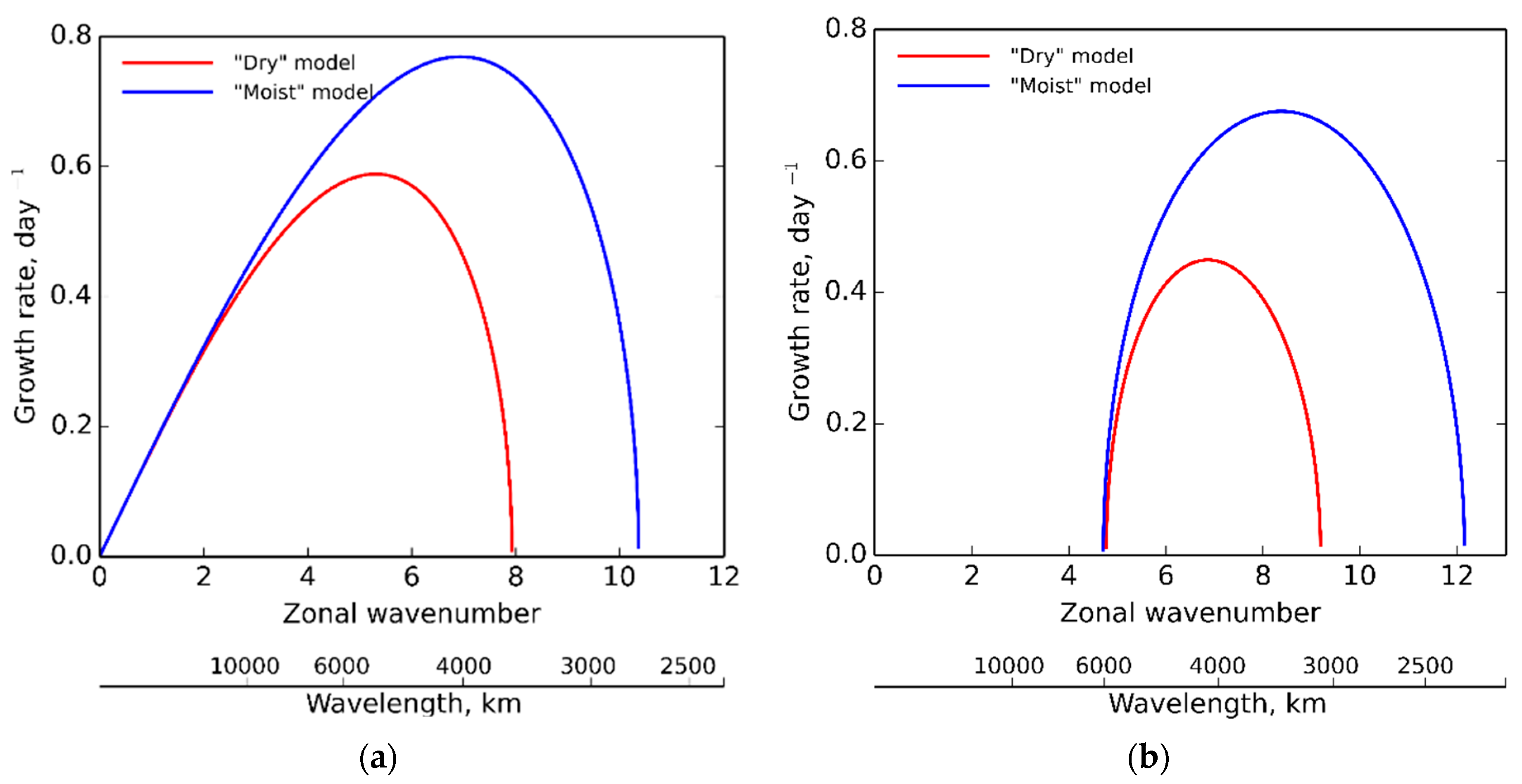
The growth rate of the unstable waves as a function of zonal wavenumber $k_z$ for the “dry” and “moist” $f$-plane and $\beta$-plane models are illustrated in Figure 1. The $f$-plane model has a short-wave cutoff. In other words, there is a critical value of wavelength $L_{min}^f$ above which instability occurs. If wavelength $L_w<L_{min}^f$ then the phase velocity is purely real and, therefore, this wave is stable, and its amplitude does not grow with time [36]. The value of $L_{min}^f$ is obtained from the condition that the discriminant ${\eta }^2-4\left(\eta \coth \eta -1\right)$ of the Equation (10) is equal to zero, which gives $\eta ={\eta }_c=2.3994$ and, therefore, $L_{min}^f\approx 3575$ km for the “dry” model, and $L_{min}^f\approx 2735$ km for the “moist” model (see

Table 1. Characteristics of baroclinic instability obtained from the f-plane and β-plane models.

Models	${\mathit{L}}_{\mathit{m}\mathit{i}\mathit{n}}^{\mathit{f}},\mathbf{km}$	${\mathit{L}}_{\mathit{m}\mathit{a}\mathit{x}}^{\mathit{f}},\mathbf{km}$	${\mathit{L}}_{\mathit{k}\mathit{c}\mathit{m}\mathit{a}\mathit{x}}^{\mathit{f}},\mathbf{km}$	${\mathit{\chi }}_{\mathit{k}},\mathbf{d}\mathbf{a}{\mathbf{y}}^{-1}$	${\mathit{t}}^{\mathit{d}},\mathbf{d}\mathbf{a}\mathbf{y}$
f-plane models:
“Dry”	3.575	-	5340	0.59	1.18
“Moist”	2735	-	4090	0.77	0.90
β-plane models:
“Dry”	3085	5945	4130	0.45	1.54
“Moist”	2333	6015	3385	0.68	1.02

Note: $t^d$ is a doubling time.

). Thus, under the influence of the atmospheric moisture, baroclinic unstable waves are shifted into the shortwave part of the spectrum.

Note that one of the disadvantages of $f$-plane model is that the long waves are unstable that contradicts, at least, the results of the numerical simulations with global models, which show that planetary-scale waves are practically stable. It is well-known that this is a consequence of the $f$-plane approximation [21]. In other words, in order to obtain a qualitatively correct result for long waves using simple models, it is needed to consider the $\beta$-effect (see Figure 1b). Examining the $\beta$-plane model, we can plot the marginal stability (neutral) curve that separates stable and unstable waves by setting the discriminant ${\beta }^2{\mu }^4+u_T^2{k}^4\left(k^4-4{\mu }^4\right)$ of the Equation (15) equal to zero. Then we can find both the shortwave cut-off $L_{min}^{\beta }$ and the longwave cut-off $L_{max}^{\beta }$. Thus, unstable waves satisfy the condition $L_{min}^{\beta }\le L_w\le L_{max}^{\beta }$. The values of $L_{min}^{\beta }$ for the “dry” and “moist” models are, respectively, 3085 and 2333 km, whereas the values of $L_{max}^{\beta }$ for the “dry” and “moist” models are of 5945 and 6015 km respectively (see Table 1).

The influence of static stability and MTG on the growth rate of baroclinic unstable waves is usually analyzed with respect to the most unstable wave, since this wave will dominate the evolutionary process of baroclinic instability [21]. The wavelength $L_{kcmax}$ of the most unstable wave corresponds to the point at which $\partial {\chi }_k/\partial k=0$. For the “dry” and “moist” versions of f-plane model the values of $L_{kcmax}^f$ are, respectively, 5340 and 4090 km, whereas for the $\beta$-plane model—4130 and 3385 km respectively. The calculated values of $L_{kcmax}$ for the “moist” versions of both the $f$-plane and $\beta$-plane models agreeing well with the observed extratropical cyclonic waves. In this regard a few clarifications are required. The two models used in this study fundamentally describe the formation of cyclones in the entire thickness of the troposphere, which is almost impossible since loss of stability usually occurs in the lower troposphere. Numerical experiments with multilayer general circulation models of the atmosphere show that the maximum growth rate of unstable modes shifts toward higher wavenumbers with $k=14,15$ ($L_w\approx 2000$ km) [87]. Since the vertical profile of these modes has a maximum in the lower troposphere, when calculating their growth rates it is necessary to take into account the energy dissipation in the atmospheric boundary layer and the turbulent dissipation due to the horizontal wind shear, which is proportional to the squared wavenumber (e.g., [47,87]). When this dissipation is taken into account in general circulation models, then the maximum of the resulting growth rate shifts again to the spectral region with wave numbers k = 6–8 ($L_w\approx$ 3500–4500 km) [87].

3.2.2. Sensitivity Functions

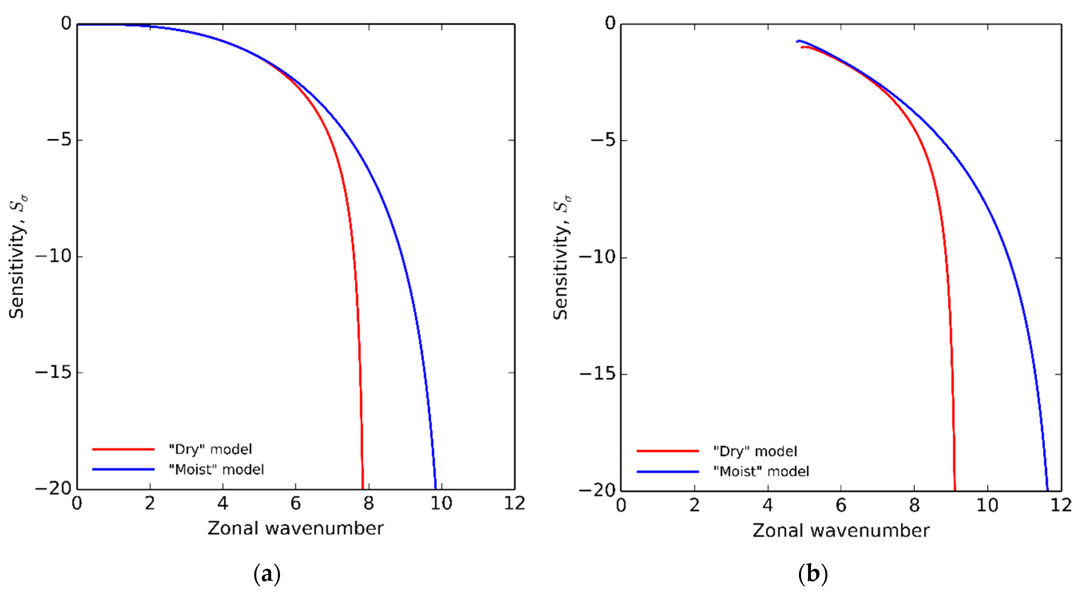
Sensitivity functions $S_{\sigma }$ with respect to the static stability parameter as functions of zonal wavenumber $k_z$ for the “dry” and “moist” f-plane and β-plane models are plotted in Figure 2. As the wavenumber increases, the absolute values of sensitivity functions $S_{\sigma }$ grow exponentially meaning that the effect due to a change in the vertical stratification of the atmosphere substantially depends on the unstable wavelength. Short waves are more affected by changes in atmospheric static stability than longer waves. Atmospheric moisture also noticeably affects the sensitivity of unstable waves to the parameter of static stability (see

Table 2. Absolute and relative sensitivity functions for the most unstable wave obtained from the f-plane and β-plane models.

Models	${\mathit{S}}_{\mathit{\sigma }}$	${\mathit{S}}_{\mathbf{\Lambda }}$	${\mathit{S}}_{{\mathit{u}}_{\mathit{T}}}$	${\mathit{S}}_{\mathit{\sigma }}^{\mathit{R}}$	${\mathit{S}}_{{\mathit{u}}_{\mathit{T}}}^{\mathit{R}}$
f-plane models:
“Dry”	−1.71	0.0196	-	−0.50	-
“Moist”	−3.84	0.0256	-	−0.50	-
β-plane models:
“Dry”	−2.47	-	0.0864	−0.94	1.44
“Moist”	−4.34	-	0.1031	−0.64	1.14

Note: $S_{\mathsf{\Lambda }}^R=1$ for all unstable waves.

). Results show that the β-plane model is more sensitive to the static stability then the f-plane model. Since sensitivity functions $S_{\sigma }$ obtained from f-plane and β-plane models are negative for all unstable waves, the increase in static stability leads to the decrease in the growth rates of unstable modes.

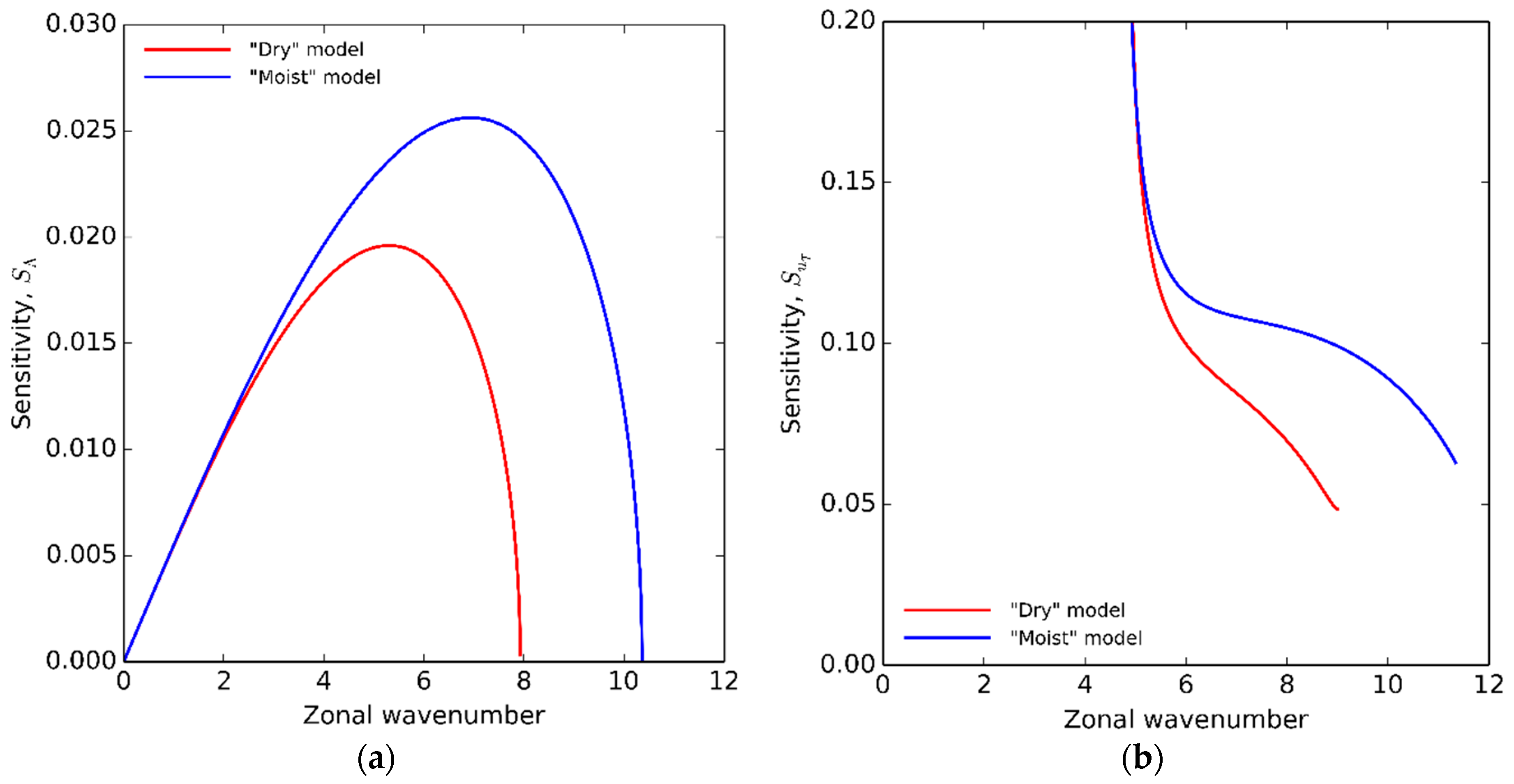
Sensitivity functions $S_{\mathsf{\Lambda }}$ and $S_{u_T}$ which represent the influence of MTG on the growth rate of unstable waves for the “dry” and “moist” f-plane and β-plane models are shown in Figure 3. From the comparison of graphs shown in Figure 1a and Figure 3a, it follows that the graph of function $S_{\mathsf{\Lambda }}$ is similar to the graph of function ${\chi }_k$. Therefore, in the f-plane model, the most unstable wave possesses the highest sensitivity to MTG, while in the β-plane model, the shorter the wave, the more sensitive it is to the horizontal temperature gradient, which is consistent with the results obtained from general circulation models of the atmosphere (e.g., [47,87]). It can be shown that the sensitivity functions $S_{\mathsf{\Lambda }}$ and $S_{u_T}$, when considered over the same domain of wavenumbers, are related by the equation $S_{\mathsf{\Lambda }}=0.25\times S_{u_T}$. Using this equation, we can compare the results obtained from both models.

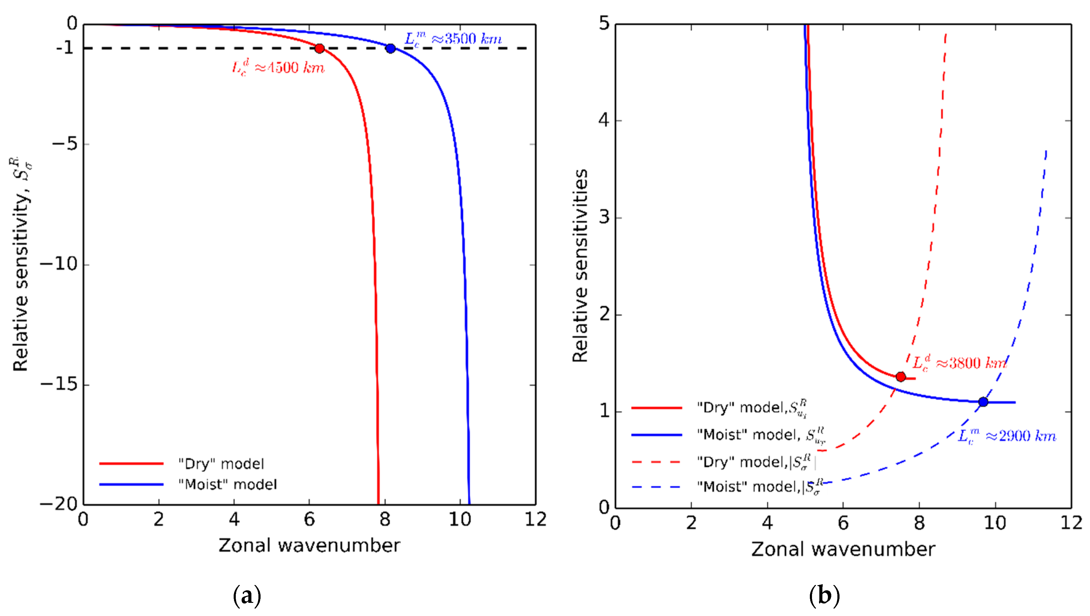
The relative importance of control parameters, the static stability parameter and MTG, in the development of baroclinic instability can be estimated using relative sensitivity functions displayed in Figure 4. The analysis of relative sensitivity functions shows that for each model (“dry” and “moist” f-plane and β-plane) there is a critical wavelength $L_c$ that splits up the wave spectrum in two regions. In the development of baroclinic instability the static stability plays more important role than the MTG for waves with $L_w<L_c$. In contrast, for waves with $L_w>L_c$ the MTG are more important than the static stability. Atmospheric moisture strongly affects the critical value $L_c$. For the “dry” (“moist”) f-plane model the critical wavelength is 4500 (3500) km, whereas for the β-plane model—3800 (2900) km.

3.2.3. Estimating Climate Change Impact on Eddy Meridional Moisture Transport

The Effect of Static Stability on Eddy Meridional Moisture Transport

In order to estimate the effect of static stability on eddy meridional moisture transport, we need to define a climate change scenario that includes estimates of both surface and upper tropospheric temperature changes. Surface temperature change is a well-studied phenomenon and thus we will use the estimate provided in the WMO report [2], according to which the average surface temperature has increased by roughly $1°\mathrm{C}$ over the last century. Temperature change in upper troposphere is significantly more uncertain given the fact that various measurement techniques (e.g., radiosondes, satellites) produce inconsistent results. For the purposes of this study, we will make use of an estimate provided in [60], which found that the increase in upper tropospheric temperature outpaces the increase in surface temperature by about $2°\mathrm{C}$ in mid-latitudes. In this scenario, the temperature lapse rate $\mathsf{\Gamma }=-dT/dz$ has decreased from the initial (base) value of 6.5 $°\mathrm{C}/\mathrm{km}$ to 6.3 $°\mathrm{C}/\mathrm{km}$. This change leads to the following dynamical effects: the temperature in the middle troposphere increases by about 1.8 °C, the dry static stability parameter also increases slightly (by about $0.7\%$). However, the effective static stability parameter ${\mathsf{\Gamma }}_{eff}$ actually demonstrates the opposite behavior: ${\mathsf{\Gamma }}_{eff}$ decreases by more than 5.4%. Thus, dry and moist models provide completely distinct results both quantitatively and qualitatively. The growth rate $k{c}_i$ of the most unstable mode obtained using the dry f-plane model decreases slightly, by about $0.2\times {10}^{-2}$ day⁻¹, which is 0.36% of the base value shown in Table 1. On the other hand, the moist f-plane model shows an increase in the growth rate $k{c}_i$ of $~2.2\times {10}^{-2}$ day⁻¹, which is ~2.8% of the base value (see Table 1). In dry β-plane model, the growth rate of the most unstable wave decreases by about $0.3\times {10}^{-2}$ day⁻¹, which is 0.7% of the base value shown in Table 1, while in the moist version of this model the growth rate increases by more than $2.4\times {10}^{-2}$ day⁻¹, which is ~3.6% of the base value. Changes in the growth rates of unstable waves cause changes in AMEMF. This effect can be estimated from the Equation (9). For the dry f-plane and β-plane models, the decrease in AMEMF is insignificant, only about 0.5% for both models, while in the moist f-plane and β-plane models there is an increase in AMEMF by about 4.5% and more than 5%, respectively. Hence the results obtained with f-plane and β-plane models are quite similar.

The Effect of Meridional Temperature Gradient on Eddy Meridional Moisture Transport

Let us now consider the effect of changes due to the global warming in the second control parameter, MTG, on the growth rate of unstable baroclinic waves and, consequently, on the AMEMF. The thermal wind equation relates MTG to the vertical wind shear, which in f-plane and β-plane models is characterized by parameters Λ and $u_T$, respectively. In general, the larger the equator-to-pole temperature difference, the stronger the resulting wind shear will be. If we know the MTG variation caused by climate change, then we can find the corresponding changes in the parameters Λ and $u_T$ by solving the thermal wind equation. In the next step, after the variations $\delta \mathsf{\Lambda }$ and $\delta u_T$ have been calculated, we can analytically estimate their influence and, therefore, the effect of MTG variations on the change in the growth rates of unstable modes by using Equations (14) and (17) and taking into account the known values of sensitivity functions $S_{\mathsf{\Lambda }}$ and $S_{u_T}$ (see Table 2). However, we first need to determine the variation in MTG caused by the climate change.

It has previously been shown that in polar areas changes in surface air temperature $T_{sfc}$ caused by a change in the planetary energy balance are greater than changes in $T_{sfc}$ in the mid-latitude and equatorial areas. Known as polar amplification, this climatic phenomenon is more profound in the northern hemisphere than in the southern hemisphere [88,89].

The earth’s energy imbalance can be caused by various natural and human factors and, in particular, by changes in the concentrations of anthropogenic greenhouse gases in the atmosphere [90,91]. As a specific example, we consider the northern hemisphere. Because of Arctic amplification, the surface air temperature at high latitudes of the northern hemisphere increased at about twice the rate of global mean surface temperature since the middle of the 20th century [92]. Arctic amplification is traced near the surface and in the lower troposphere, weakening MTG and, thus, reducing the vertical wind shear and contributing to the weakening of the westerly mid-latitude jet stream. In the upper and middle troposphere, however, climate change enhances MTG, thereby increasing the vertical wind shear and contributing to strengthening the zonal flow [93,94,95,96]. Exploration of historic trends in the upper-tropospheric vertical wind shear in the North Atlantic region based on three independently created reanalysis datasets has shown that in the area of interest the vertical wind shear has increased by about 15% over the last few decades [94].

As noted in [94], a stronger MTG and a correspondingly stronger vertical wind shear in the upper troposphere are masked by a weaker MTG and a correspondingly weaker vertical wind shear in the lower troposphere. Climate modeling results show that changes in the upper-tropospheric MTG play a primary role in the formation of large-scale atmospheric dynamics at mid-latitudes, affecting the intensity of vertical wind shear and zonal flow, while changes in the lower tropospheric MTG play a secondary role [97,98]. The annual-mean equator-to-pole temperature difference over the troposphere is about 40 °C, so the average tropospheric MTG is about 4 $°\mathrm{C}$ per 1000 km [99]. However, MTG varies with latitude. The strongest MTG is concentrated in the middle latitudes, contributing to the formation of the so-called upper tropospheric frontal zone and the associated zonal flow, the speed of which increases with height [20,99]. In this study, we have assumed that the vertical wind shear parameter Λ used in f-plane model is 30 ms⁻¹ bar⁻¹ [21,42]. Accordingly, the parameter $u_T$ that characterises the vertical wind shear in β-plane model is 7.5 ms⁻¹. This vertical wind shear is associated with an upper-tropospheric frontal zone which in our case extends over the entire thickness of the troposphere and has an MTG of $~7.54°\mathrm{C}$ per 1000 km. Note that in well-developed upper-tropospheric frontal zones, the temperature contrast can reach 11–12 °C per 1000 km in mid-latitudes.

Based on preceding discussion, when determining the MTG value, we assume that climate change weakens the annual MTG in the lower troposphere through more significant heating of higher latitudes, whereas in the upper troposphere MTG increases because of a strong upper-tropospheric warming of lower latitudes. For a climate change scenario discussed in this paper, the response of the mass-weighted vertically averaged annual mean MTG to increase in the surface temperature by $1°\mathrm{C}$ is about $-0.2°\mathrm{C}$ per 1000 km, which is ~2.7% of the base value. Accordingly, this change in MTG generates the following variations in the parameters $\mathsf{\Lambda }$ and $u_T$ that characterize the vertical wind shear: $\delta \mathsf{\Lambda }=+0.8{\mathrm{ms}}^{-1}{\mathrm{bar}}^{-1}$ and $\delta u_T=+0.2$ ${\mathrm{ms}}^{-1}$. Next we can estimate the influence of $\delta \mathsf{\Lambda }$ and $\delta u_T$ on the growth rate of the most unstable mode $k{c}_i$ using Equations (12) and (18). Values for sensitivity functions $S_{\mathsf{\Lambda }}$ and $S_{u_T}$ used in this equation are shown in Table 2. Calculations show that the growth rate $k{c}_i$ obtained from the dry f-plane model increases by $~0.016$ day⁻¹. In turn, the growth rate obtained from the moist f-plane model increases by $~0.020$ day⁻¹, however, in relative terms, this increase is also 2.7% of the base value since the base growth rate is larger in the moist model than in the dry model. The β-plane model yields fairly similar results. In the dry version of this model, $k{c}_i$ increases by $~0.017$ day⁻¹, which is about 4% of the base value, and in the moist version by $~0.021$ day⁻¹, which is 3.1% of the base value. Now, we can estimate the effect of MTG change on the meridional moisture transport using the Equation (9) and the obtained values of $\Delta \left(k{c}_i\right)$. The AMEMF calculated using dry f-plane and β-plane models increases by 3.2% and 4.2%, respectively. In turn, increases in the meridional moisture flux obtained from the moist f-plane and β-plane models are 3.5% and 4.2% respectively.

4. Discussion

In summary, using the two classic atmospheric models, mid-latitude f-plane, and β-plane models, for baroclinic instability we have estimated the climate change impact on the mid-latitude moisture transport. Fundamental dynamical parameters, static stability parameter, and MTG, were used as indicators of climate change, and the static stability parameter was calculated both with and without considering the atmospheric moisture (“moist” and “dry” models respectively). We have shown that neglecting atmospheric moisture in the calculation of static stability parameter (in other words, the use of the dry static stability parameter instead of the effective static stability parameter) leads to tangible differences between the results obtained using dry and moist models. Because of the climate change, the dry static stability parameter slightly increases, weakening AMEMF only insignificantly (by less than 0.5%). At the same time, the effective static stability parameter decreases causing an intensification of baroclinic instability and, consequently, an increase in AMEMF of about 5%.

In addition to affecting the static stability of the atmosphere, climate change also affects the MTG, which is one of the main fundamental dynamical parameters that “controls” the global atmospheric circulation and the eddy meridional moisture transport. Although the changes in MTG in the lower troposphere and the upper troposphere have opposite signs, the mass-weighted vertically averaged annual-mean MTG increases under global warming. This leads to an enhanced vertical wind shear producing more favorable conditions for the development of baroclinic instability and generation of large-scale atmospheric eddies that transport moisture from low to high latitudes. According to the climate change scenario discussed here, the response of the mass-weighted vertically averaged annual mean MTG to an increase in the surface temperature of $1°\mathrm{C}$ is about $-0.2°\mathrm{C}$ per 1000 km, which is ~2.7% of the base value. In turn, under this change in MTG the parameters $\mathsf{\Lambda }$ and $u_T$, which characterize the vertical wind shear, also increase by 0.8 ${\mathrm{ms}}^{-1}{\mathrm{bar}}^{-1}$ and $0.2$ ${\mathrm{ms}}^{-1}$ respectively, thereby strengthening the eddy meridional moisture transport by about 4%.

Suppose that the static stability of the atmosphere and the MTG are independent of each other, or in other words, suppose that these parameters change independently of one other under the influence of climate change. Then, from the moist models (models with effective static stability parameter), it can be estimated that an increase in near-surface temperature by $1°\mathrm{C}$ leads to an increase in AMEMF of about 9% compared with the reference climate state.

However, since the effect of static stability is negligible in dry models, an increase in AMEMF is solely attributable to a change in the MTG. The assumption that the parameters are independent of each other is fairly often used in the sensitivity analysis of systems when considering the influence of infinitesimal parameter variations on model variables. This approach is referred to as “One-factor-at-a-time” (OAT). In our case, the use of this approach is quite reasonable, since we are studying the effects of infinitesimal variations caused by climate change in the static stability parameter and the MTG on the growth rate of unstable baroclinic waves and, hence, on the AMEMF. The sensitivity functions obtained represent an efficient tool for estimating the impact of various climate change scenarios on changes in the AMEMF

In the climate change scenario being considered, the temperature of lower troposphere, in which the atmospheric moisture is concentrated, increases by about $1.5°\mathrm{C}$. This leads to an increase in specific humidity of about 10.5%. Thus, since both AMEMF and atmospheric water vapor content increase under this scenario, a rather noticeable restructuring of the global water cycle is expected. For instance, in middle and high latitudes, the meridional moisture transport enhanced due to the global warming may lead to more precipitation overall as well as changes in the intensity and frequency of heavy rainfall events increasing the likelihood of flooding, particularly in coastal areas.

In this study, we applied an idealized framework to estimate the response of AMEMF to changes that occur in the earth’s climate system under global warming. Undoubtedly, the results obtained from simplified models should be approached with caution. Ideally, further studies are required to simulate climate change impact on the global hydrological cycle using more complex climate models with full physics and high resolution. However, this problem is quite costly in terms of computational resources, so obtaining estimates using a simplified (classical) framework is very useful for better understanding the fundamentals of thermodynamic effects of climate change.

References

- IPCC. Climate Change 2013: The Physical Science Basis. Contribution of Working Group I to the Fifth Assessment Report of the Intergovernmental Panel on Climate Change; Stocker, T.F., Qin, D., Plattner, G.-K., Tignor, M., Allen, S.K., Boschumg, J., Nauels, A., Xia, Y., Bex, V., Midgley, P.M., Eds.; Cambridge University Press: Cambridge, UK; New York, NY, USA, 2013; p. 1535. [Google Scholar]
- WMO. Statement on the State of the Global Climate in 2018; WMO-No. 1233; World Meteorological Organization: Geneva, Switzerland, 2019; p. 39. [Google Scholar]
- Fanglin, Y.; Arun, K.; Schlesinger, M.E.; Wang, W. Intensity of hydrological cycles in warmer climates. J. Clim. 2003, 16, 2419–2423. [Google Scholar]
- Huntington, T.G. Evidence for intensification of the global water cycle: Review and synthesis. J. Hydrol. 2006, 319, 83–95. [Google Scholar] [CrossRef]
- Held, I.M.; Soden, B.J. Robust response of the hydrological cycle to global warming. J. Clim. 2006, 19, 5686–5699. [Google Scholar] [CrossRef]
- Bengtsson, L. The global atmospheric water cycle. Environ. Res. Lett. 2010, 5, 025002. [Google Scholar] [CrossRef]
- Grover, V.I. Impact of Climate Change on Water and Health; CRC Press: Boca Raton, FL, USA, 2012; p. 426. [Google Scholar]
- Durack, P.J.; Wijffels, S.E.; Matear, R.J. Ocean salinities reveal strong global cycle intensification during 1950–2000. Science 2012, 336, 455–458. [Google Scholar] [CrossRef]
- Bosilovich, M.G.; Robertson, F.R.; Chen, J. Global energy and water budgets in MERRA. J. Clim. 2011, 24, 5721–5739. [Google Scholar] [CrossRef]
- Trenberth, K.E.; Fasullo, J.T. North American water and energy cycles. Geophys. Res. Lett. 2013, 40, 365–369. [Google Scholar] [CrossRef]
- Djebou, D.C.S.; Singh, V.P. Impact of climate change on the hydrologic cycle and implications for society. Environ. Soc. Psychol. 2016, 1, 36–49. [Google Scholar] [CrossRef]
- Wentz, F.J.; Ricciardulli, L.; Hilburn, K.; Mears, C. How Much More Rain Will Global Warming Bring? Science 2007, 317, 233–235. [Google Scholar] [CrossRef]
- Schmidt, G.A.; Ruedy, R.A.; Miller, R.L.; Lacis, A.A. Attribution of the present-day total greenhouse effect. J. Geophys. Res. 2010, 115, D20106. [Google Scholar] [CrossRef]
- Chou, C.; Lan, C.-W. Changes in the annual range of precipitation under global warming. J. Clim. 2012, 25, 222–235. [Google Scholar] [CrossRef]
- Behrangi, A.; Christens, M.; Richardson, M.; Lebsock, M.; Stephens, G.; Huffman, G.J.; Bolvin, D.; Adler, R.F.; Gardner, A.; Lambrigtsen, B.; et al. Status of high-latitude precipitation estimates from observations and reanalyses. J. Geophys. Res. Atmos. 2016, 121, 4468–4486. [Google Scholar] [CrossRef]
- O’Gorman, P.A.; Schneider, T. The physical basis for increases in precipitation extremes in simulations of 21st century climate change. Proc. Natl. Acad. Sci. USA 2016, 106, 14773–14777. [Google Scholar] [CrossRef]
- Putnam, A.E.; Broecker, W.S. Human-induced changes in the distribution of rainfall. Sci. Adv. 2017, 3, e1600871. [Google Scholar] [CrossRef]
- Giorgi, F.; Raffaele, F.; Coppola, E. The response of precipitation characteristics to global warming from climate projections. Earth Syst. Dyn. 2019, 10, 73–89. [Google Scholar] [CrossRef]
- Held, I.M.; Hoskins, B.J. Large-scale eddies and the general circulation of the atmosphere. Adv. Geophys. 1985, 28, 3–31. [Google Scholar] [CrossRef]
- Matveev, L.T. The Theory of General Circulation of the Atmosphere and Earth’s Climate; Hydrological and Meteorological Publisher: Leningrad, Russia, 1991; p. 296. [Google Scholar]
- Holton, J.R.; Hakim, G.J. Introduction to Dynamic Meteorology, 5th ed.; Elsevier: Amsterdam, The Netherlands, 2012; p. 552. [Google Scholar]
- Vallis, G.K. Atmospheric and Oceanic Fluid Dynamics: Fundamentals and Large-Scale Circulation; Cambridge University Press: Cambridge, UK, 2006; p. 745. [Google Scholar]
- Randall, D. An Introduction to the Global Circulation of the Atmosphere; Princeton University Press: Princeton, NJ, USA, 2015; p. 456. [Google Scholar]
- Lindzen, R.S. Dynamics in Atmospheric Physics; Cambridge University Press: Cambridge, UK, 1990; p. 320. [Google Scholar]
- Gimeno, L.; Dominguez, F.; Nieto, R.; Trigo, R.; Drumond, A.; Reason, C.J.C.; Taschetto, A.; Ramos, A.M.; Kumar, R.; Marengo, J. Major mechanisms of atmospheric moisture transport and their role in extreme precipitation events. Annu. Rev. Environ. Resour. 2016, 41, 117–141. [Google Scholar] [CrossRef]
- Zhang, Z.; Ralph, F.M.; Zheng, M. The relationship between extratropical cyclone strength and atmospheric river intensity and position. Geophy. Res. Lett. 2018, 46, 1814–1823. [Google Scholar] [CrossRef]
- Lambert, S.J. The effect of enhanced greenhouse warming on winter cyclone frequencies and strengths. J. Clim. 1995, 8, 1447–1462. [Google Scholar] [CrossRef]
- Geng, Q.; Sugi, M. Possible change of extratropical cyclone activity due to enhanced greenhouse gases and sulphate aerosols: Study with a high-resolution AGCM. J. Clim. 2003, 16, 2262–2274. [Google Scholar] [CrossRef]
- Fyfe, J.C. Extratropical Southern Hemisphere cyclones: Harbingers of climate change. J. Clim. 2003, 16, 2802–2805. [Google Scholar] [CrossRef]
- Yin, J.H. A consistent poleward shift of the storm tracks in simulations of 21st century climate. Geophys. Res. Lett. 2005, 32. [Google Scholar] [CrossRef]
- Lambert, S.J.; Fyfe, J.C. Changes in winter cyclone frequencies and strengths simulated in enhanced greenhouse warming experiments: Results from the models participating in the IPCC diagnostic exercise. Clim. Dyn. 2006, 26, 713–728. [Google Scholar] [CrossRef]
- Bengtsson, L.; Hodges, K.I.; Roeckner, E. Storm tracks and climate change. J. Clim. 2006, 19, 3518–3543. [Google Scholar] [CrossRef]
- Wu, Y.; Ting, M.; Seager, R.; Huang, H.-P.; Cane, M.A. Changes in storm tracks and energy transports in a warmer climate simulated by the GFDL CM2.1model. Clim. Dyn. 2011, 37, 53–72. [Google Scholar] [CrossRef]
- Pfahl, S.; O’Gorman, P.A.; Singh, M.S. Extratropical cyclones in idealized simulations of changed climates. J. Clim. 2015, 28, 9373–9392. [Google Scholar] [CrossRef]
- Charney, J.G. The dynamics of long waves in a baroclinic westerly current. J. Meteorol. 1947, 4, 136–162. [Google Scholar] [CrossRef]
- Eady, E.T. Long waves and cyclone waves. Tellus 1949, 1, 33–52. [Google Scholar] [CrossRef]
- Phillips, N.A. Energy transformations and meridional circulations associated with simple baroclinic waves in a two-level, quasi-geostrophic model. Tellus 1954, 6, 273–286. [Google Scholar] [CrossRef]
- Schultz, D.M.; Bosart, L.F.; Colle, B.A.; Davies, H.C.; Dearden, C.; Keyser, D.; Martius, O.; Roebber, P.J.; Steenburgh, W.J.; Volkert, H.; et al. Extratropical Cyclones: A Century of Research on Meteorology’s Centerpiece. AMS Meteorol. Monogr. 2018, 59, 1–56. [Google Scholar] [CrossRef]
- Lorenz, E.N. Available potential energy and the maintenance of the general circulation. Tellus 1955, 7, 157–167. [Google Scholar] [CrossRef]
- Oort, A.H.; Peixoto, J.P. The annual cycle of the energetics of the atmosphere on a planetary scale. J. Geophys. Res. 1974, 79, 2705–2719. [Google Scholar] [CrossRef]
- Oort, A.H. Global Atmospheric Circulation Statistics, 1958–1973; No. 14; US Department of Commerce; National Oceanic and Atmospheric Administration: Washington, DC, USA, 1983; pp. 180–226.
- Dynmikov, V.P. Development of baroclinic instability in an atmosphere with a variable static stability parameter. Atmos. Ocean. Phys. 1978, 14, 352–356. [Google Scholar]
- Grotjahn, R. Baroclinic Instability. In Encyclopedia of Atmospheric Sciences; Holton, J.R., Curry, J.A., Pyle, J.A., Eds.; Academic Press: Cambridge, MA, USA, 2003; pp. 419–467. [Google Scholar]
- Lambaerts, J.; Lapeyre, G.; Zeitlin, V. Moist versus dry baroclinic instability in a simplified two-layer atmospheric model with condensation and latent heat release. J. Atmos. Sci. 2012, 69, 1405–1426. [Google Scholar] [CrossRef] [Green Version]
- O’Gorman, P.A. The effective static stability experiences by eddies in a moist atmosphere. J. Atmos. Sci. 2011, 68, 75–90. [Google Scholar] [CrossRef]
- Soldatenko, S.A. Numerical modelling of wave cyclogenesis in a moist baroclinic atmosphere. Meteorol. Hydrol. 1989, 7, 5–14. [Google Scholar]
- Matveev, L.T.; Soldatenko, S.A. Effect of heat of condensation on the spectral energy distribution of baroclinically unstable modes. Earth Sci. Sect. 1989, 306, 70–74. [Google Scholar]
- Kuo, Y.-H.; Shapiro, M.A.; Donall, E.G. The interaction between baroclinic and diabatic processes in a numerical simulation of a rapidly intensifying extratropical marine cyclone. Mon. Weather Rev. 1991, 119, 368–384. [Google Scholar] [CrossRef] [Green Version]
- Stoelinga, M.T. A potential vorticity-based study of the role of diabatic heating and friction in a numerically simulated baroclinic cyclone. Mon. Weather Rev. 1996, 124, 849–874. [Google Scholar] [CrossRef] [Green Version]
- Büeler, D.; Pfahl, S. Potential vorticity diagnostics to quantify effects of latent heating in extratropical cyclones. Part I: Methodology. J. Atmos. Sci. 2017, 74, 3567–3590. [Google Scholar] [CrossRef]
- Letcher, T.M. Climate Change. In Observed Impacts on Planet Earth; Elsevier: Amsterdam, The Netherlands, 2009; p. 492. [Google Scholar]
- Shepherd, T.G. Atmospheric circulation as a source of uncertainty in climate change projections. Nat. Geosci. 2015, 7, 703–708. [Google Scholar] [CrossRef]
- Mann, M.E.; Rahmstorf, S.; Kornhuber, K.; Steinman, B.A.; Miller, S.K. Influence of anthropogenic climate change on planetary wave resonance and extreme weather events. Sci. Rep. 2017, 7, 45242. [Google Scholar] [CrossRef] [PubMed] [Green Version]
- Screen, J.A.; Bracegirdle, T.J.; Simmonds, I. Polar climate change as manifest in atmospheric circulation. Curr. Clim. Chang. Rep. 2018, 4, 383–395. [Google Scholar] [CrossRef] [PubMed] [Green Version]
- Bathiany, S.; Dakos, V.; Scheffer, M.; Lenton, T.M. Climate models predict increasing temperature variability in poor countries. Sci. Adv. 2018, 4, eaar5809. [Google Scholar] [CrossRef] [PubMed] [Green Version]
- Totz, S.; Petri, S.; Lehmann, J.; Peukert, E.; Coumou, D. Exploring the sensitivity of Northern Hemisphere atmospheric circulation to different surface temperature forcing using a statistical-dynamical atmospheric model. Nonlinear Process. Geophys. 2019, 26, 1–26. [Google Scholar] [CrossRef]
- Lee, S. A theory for polar amplification from a general circulation perspective. Asia-Pac. J. Atmos. Sci. 2014, 50, 31–43. [Google Scholar] [CrossRef]
- Pithan, F.; Thorsten, M. Arctic amplification dominated by temperature feedbacks in contemporary climate models. Nat. Geosci. 2014, 7, 181–184. [Google Scholar] [CrossRef]
- Hernandez-Deckers, D.; Von Storch, J.-S. Impact of the warming patterns on global energetics. J. Clim. 2012, 25, 5223–5240. [Google Scholar] [CrossRef]
- Frierson, D.M.W. Robust increases in midlatitude static stability in simulations of global warming. Geophys. Res. Lett. 2006, 33, L24816. [Google Scholar] [CrossRef] [Green Version]
- Chou, C.; Wu, T.-C.; Tan, P.-H. Changes in gross moist stability in the tropics under global warming. Clim. Dyn. 2013, 41, 2481–2496. [Google Scholar] [CrossRef]
- Shi, X.; Durran, D. Sensitivities of extreme precipitation to global warming are lower over mountains than over oceans and plains. J. Clim. 2016, 29, 4779–4791. [Google Scholar] [CrossRef]
- Karamperidou, C. Surface temperature gradients as diagnostic indicators of midlatitude circulation dynamics. J. Clim. 2012, 25, 4154–4171. [Google Scholar] [CrossRef] [Green Version]
- Meleshko, V.P.; Johannessen, O.M.; Baidin, A.V.; Pavlova, T.V.; Govorkova, V.A. Arctic amplification: Does it impact the polar jet stream? Tellus A 2016, 68, 32330. [Google Scholar] [CrossRef] [Green Version]
- Arndt, N. Hydrosphere. In Encyclopedia of Astrobiology; Amils, R., Ed.; Springer: Berlin/Heidelberg, Germany, 2014. [Google Scholar] [CrossRef]
- Kundzewicz, Z.W. Hydrosphere. In Encyclopedia of Ecology; Jørgensen, S.E., Fath, B.D., Eds.; Elsevier: Amsterdam, The Netherlands, 2008; pp. 1923–1930. [Google Scholar]
- Matveev, L.T. Cloud Dynamics; Springer: Cham, The Netherlands, 1984; p. 356. [Google Scholar]
- Hartmann, D.L. Global Physical Climatology; Academic Press: San Diego, CA, USA, 1994; p. 411. [Google Scholar]
- Trenberth, K.E.; Fasulo, J.T.; Kiehl, J. Earth’s global energy budget. Bull. Amer. Met. Soc. 2009, 90, 311–323. [Google Scholar] [CrossRef]
- Goosse, H.; Barriat, P.Y.; Lefebvre, W.; Loutre, M.F.; Zunz, V. Introduction to Climate Dynamics and Climate Modeling. 2008–2010. Available online: http://www.climate.be/textbook (accessed on 2 July 2019).
- Lacis, A.A.; Hansen, J.E.; Russell, G.L.; Oinas, V.; Jonas, J. The role of long-lived greenhouse gases as principal LW control knob that governs the global surface temperature for past and future climate change. Tellus B 2013, 65, 19734. [Google Scholar] [CrossRef]
- Matveev, Y.L.; Matveev, L.T.; Soldatenko, S.A. Global Cloud Fields; Hydrometeoizdat: Leningrad, Russia, 1986; p. 279. [Google Scholar]
- Peixoto, J.P.; Oort, A.H. Physics of Climate, 1st ed.; American Institute of Physics: College Park, MD, USA, 1992; p. 520. [Google Scholar]
- Naakka, T.; Nygård, T.; Vihma, T.; Sedlar, J.; Graversen, R. Atmospheric moisture transport between mid-latitudes and the Arctic: Regional, seasonal and vertical distributions. Int. J. Clim. 2019, 39, 2862–2879. [Google Scholar] [CrossRef]
- Tsukernik, M.; Lynch, A. Atmospheric meridional moisture flux over the Southern Ocean: A story of the Amundsen Sea. J. Clim. 2013, 26, 8055–8064. [Google Scholar] [CrossRef]
- Dufour, A.; Zolina, O.; Gulev, S.K. Atmospheric moisture transport to the Arctic: Assessment of reanalyses and analysis of transport components. J. Clim. 2016, 29, 5061–5081. [Google Scholar] [CrossRef]
- Trenberth, K.E.; Stepaniak, D.P. Covariability of components of poleward atmospheric energy transports on seasonal and interannual timescales. J. Clim. 2003, 16, 3691–3705. [Google Scholar] [CrossRef]
- Wetzel, A.N.; Smith, L.M.; Stechmann, S.N. Moisture transport due to baroclinic waves: Linear analysis of precipitating quasi-geostrophic dynamics. Math. Clim. Weather 2017, 3, 28–50. [Google Scholar] [CrossRef] [Green Version]
- Soldatenko, S. Influence of atmospheric static stability and meridional temperature gradient on the growth in amplitude of synoptic-scale unstable waves. Atmos. Ocean. Phys. 2014, 50, 554–561. [Google Scholar] [CrossRef]
- Soldatenko, S.A.; Chichkine, D. Climate Model Sensitivity with Respect to Parameters and External Forcing. In Topics in Climate Modeling; Hromadka, T., Rao, P., Eds.; Intech Open: Rijeka, Croatia, 2016; pp. 105–135. [Google Scholar] [CrossRef] [Green Version]
- Gastineau, G.; Soden, B.J. Model projected changes of extreme wind events in response to global warming. Geophys. Res. Lett. 2009, 36, L10810. [Google Scholar] [CrossRef] [Green Version]
- Schneider, T.; Mbengue, C. Storm-track shifts under climate change: Toward a mechanistic understanding using baroclinic mean available potential energy. J. Atmos. Sci. 2017, 74, 93–110. [Google Scholar]
- Chemke, R. Atmospheric energy transfer response to global warming. Q. J. R. Meteorol. Soc. 2017, 143, 2296–2308. [Google Scholar] [CrossRef]
- Akperov, M.G.; Mokhov, I.I. Estimates of the sensitivity of cyclonic activity in the troposphere of extratropical latitudes to changes in the temperature regime. Atmos. Ocean. Phys. 2013, 49, 129–136. [Google Scholar] [CrossRef]
- Mokhov, I.I.; Doronina, T.N.; Gryanik, V.M.; Khairullin, R.R.; Korovkina, L.V.; Lagun, V.E. Extratropical Cyclones and Anticyclones: Tendencies of Changes. In the Life Cycles of Extratropical Cyclones; Gronas, S., Hapiro, M.A., Eds.; Geophysical Institute, University of Bergen: Bergen, Norway, 1994; pp. 56–60. [Google Scholar]
- Mokhov, I.I.; Mokhov, O.I.; Petukhov, V.K. Influence of global climate change on the vortex activity of the atmosphere. Atmos. Ocean. Phys. 1992, 28, 11–26. [Google Scholar]
- Dymnikov, V.P.; Fomenko, A.A. On the spectral distribution of unstable modes in the general atmospheric circulation model. Atmos. Ocean. Phys. 1981, 17, 675–679. [Google Scholar]
- Budyko, M.I. The effect of solar radiation variations on the climate of the Earth. Tellus 1969, 21, 611–619. [Google Scholar] [CrossRef] [Green Version]
- Harvey, B.; Shaffrey, L.; Woollings, T. Equator-to-pole temperature differences and the extra-tropical storm track responses of the CMIP5 climate models. Clim. Dyn. 2014, 43, 1171–1182. [Google Scholar] [CrossRef] [Green Version]
- Hansen, J.; Sato, M.; Kharecha, P.; von Schuckmann, K. Earth’s energy imbalance and implications. Atmos. Chem. Phys. 2011, 11, 13421–13449. [Google Scholar] [CrossRef] [Green Version]
- Von Schuckmann, K.; Palmer, M.D.; Trenberth, K.E.; Cazenave, A.; Chambers, D.; Champollion, M.; Hansen, J.; Josey, S.A.; Loeb, N.; Mathieu, P.-P.; et al. An imperative to monitor Earth’s energy imbalance. Nat. Clim. Chang. 2016, 6, 138–144. [Google Scholar] [CrossRef] [Green Version]
- Cohen, J.; Screen, J.A.; Furtado, J.C.; Barlow, M.; Whittleston, D.; Coumou, D.; Francis, J.; Dethloff, K.; Entekhabi, D.; Overland, J.; et al. Recent Arctic amplification and extreme mid-latitude weather. Nat. Gensci. 2014, 7, 627–637. [Google Scholar] [CrossRef] [Green Version]
- Walsh, J.E. Intensified warming of the Arctic: Causes and impacts on middle latitudes. Glob. Planet. Chang. 2014, 117, 52–63. [Google Scholar] [CrossRef]
- Lee, S.H.; Williams, P.D.; Frame, T.H.A. Increased shear in the North Atlantic upper-level jet stream over the past four decades. Nature 2019, 572, 639–642. [Google Scholar] [CrossRef] [PubMed]
- Lorenz, D.; DeWeaver, E.T. Tropopause height and zonal wind response to global warming in the IPCC scenario integrations. J. Geophys. Res. 2007, 112. [Google Scholar] [CrossRef] [Green Version]
- Hassanzadeh, P.; Kuang, Z.; Farre, B.F. Responses of midlatitude blocks and wave amplitude to changes in the meridional temperature gradient in an idealized dry GCM. Geophys. Res. Lett. 2014, 41, 5223–5232. [Google Scholar] [CrossRef]
- Francis, J.A.; Vavrus, S.J. Evidence linking Arctic amplification to extreme weather in mid-latitudes. Geophys. Res. Lett. 2012, 39, L06801. [Google Scholar] [CrossRef]
- Yuval, J.; Kaspri, Y. Eddy activity sensitivity to changes in the vertical structure of baroclinicity. J. Atmos. Sci. 2016, 73, 1709–1726. [Google Scholar] [CrossRef]
- Marshall, J.; Plumb, R.A. Atmosphere, Ocean and Climate Dynamics: An Introductory Text; International Geophysics Series; Academic Press: Cambridge, MA, USA, 2007; p. 344. [Google Scholar]
Figure 1.
Growth rate as a function of zonal wavenumber for the “dry” and “moist” (a) f-plane and (b) β-plane models, as described by Equations (10) and (15) respectively.
Figure 2.
Sensitivity functions with respect to the static stability parameter as functions of the zonal wavenumber for the “dry” and “moist” (a) f-plane and (b) β-plane models.
Figure 3.
Sensitivity functions with respect to the meridional temperature gradient (MTG) parameter versus zonal wavenumbers for the “dry” and “moist” (a) f-plane and (b) β-plane models.
Figure 4.
Relative sensitivity functions versus zonal wavenumbers for the “dry” and “moist” (a) f-plane and (b) β-plane models.