The Influence of Environmental Change (Crops and Water) on Population Redistribution in Mexico and Ethiopia


Abstract
:1. Introduction
2. Data and Methods
2.1. Data
2.1.1. Population Redistribution
2.1.2. Built-Up
2.1.3. Climate Change Impacts
2.2. Methods
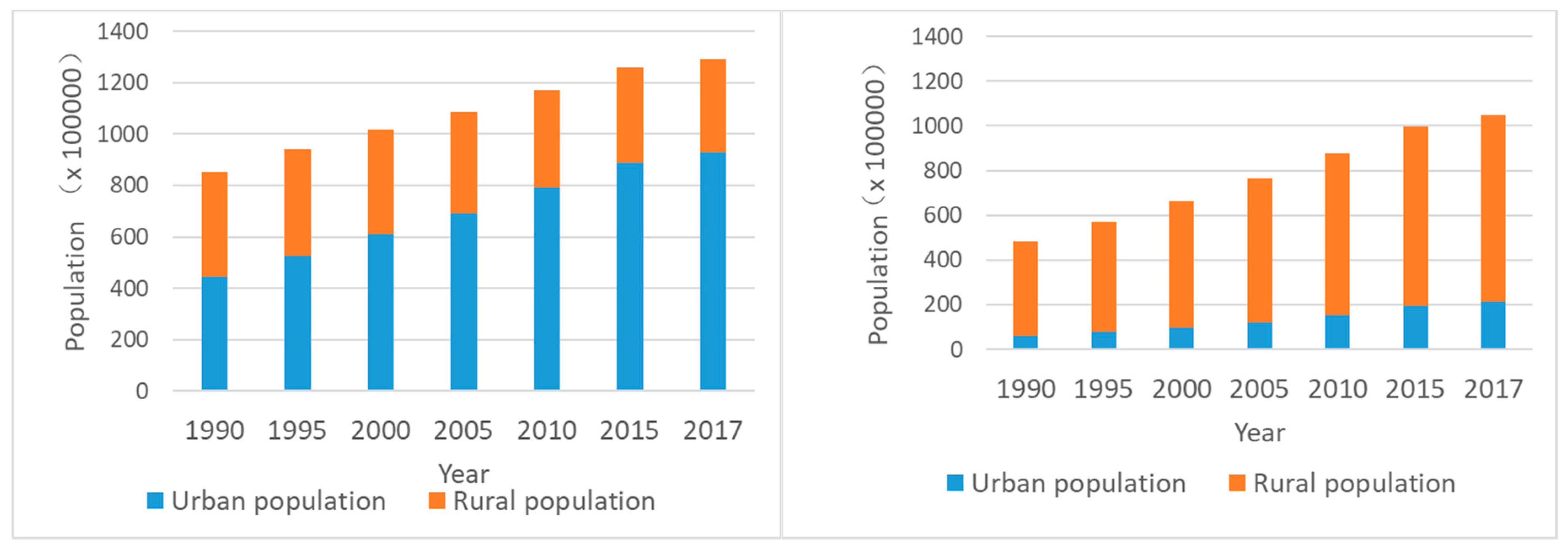
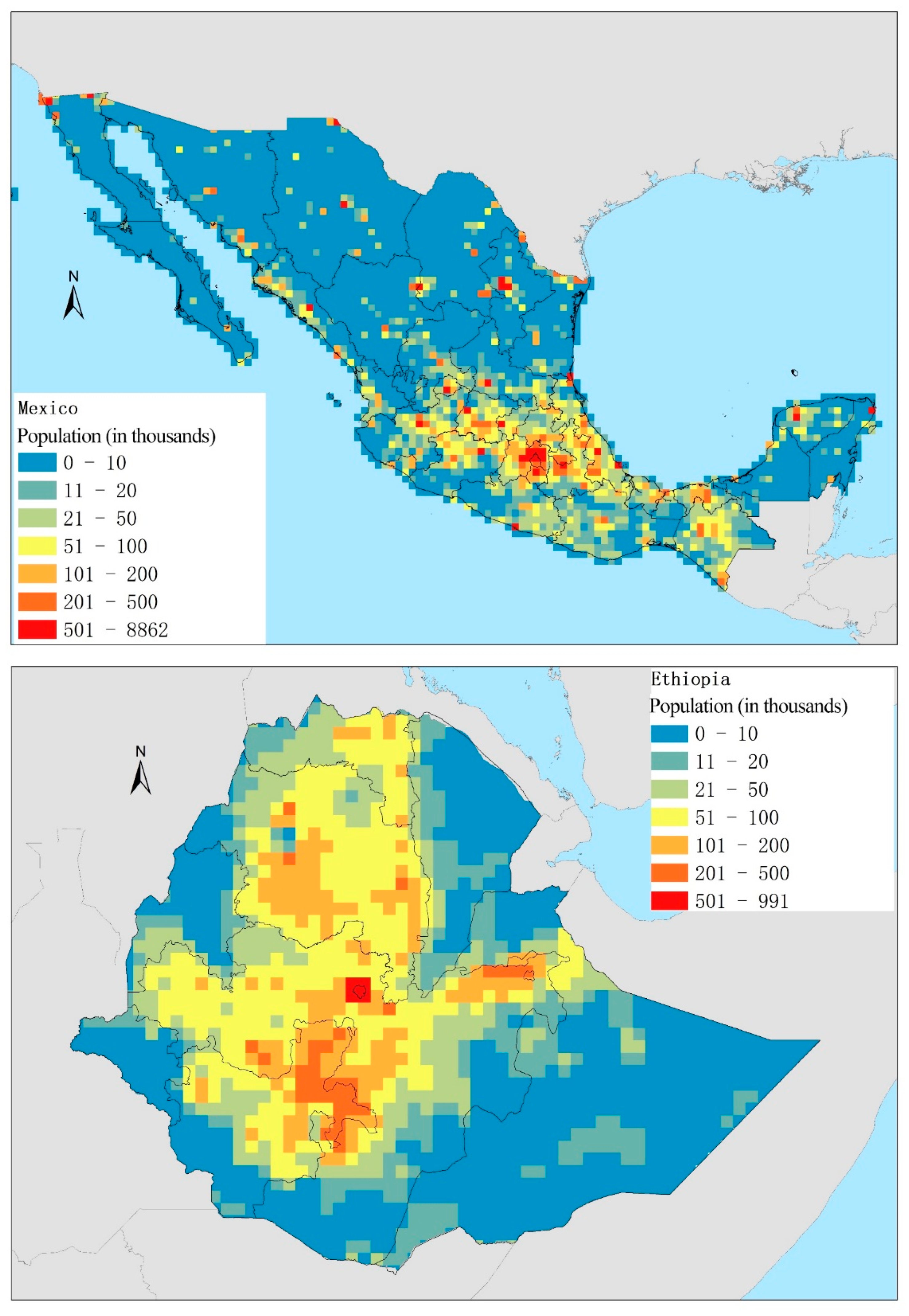
3. Case Study Countries
4. Analysis
4.1. Correlation Analysis
4.2. OLS Results
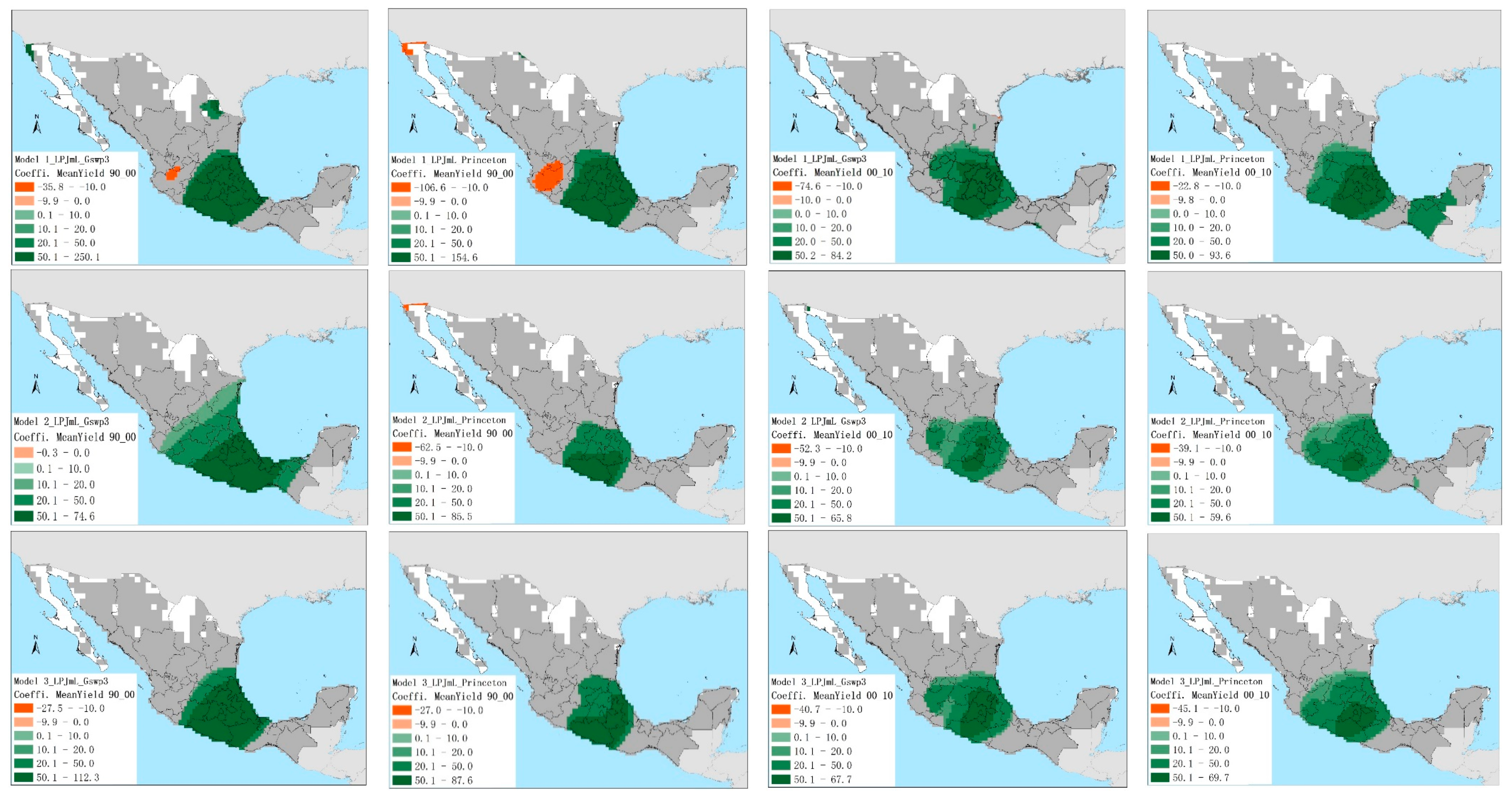
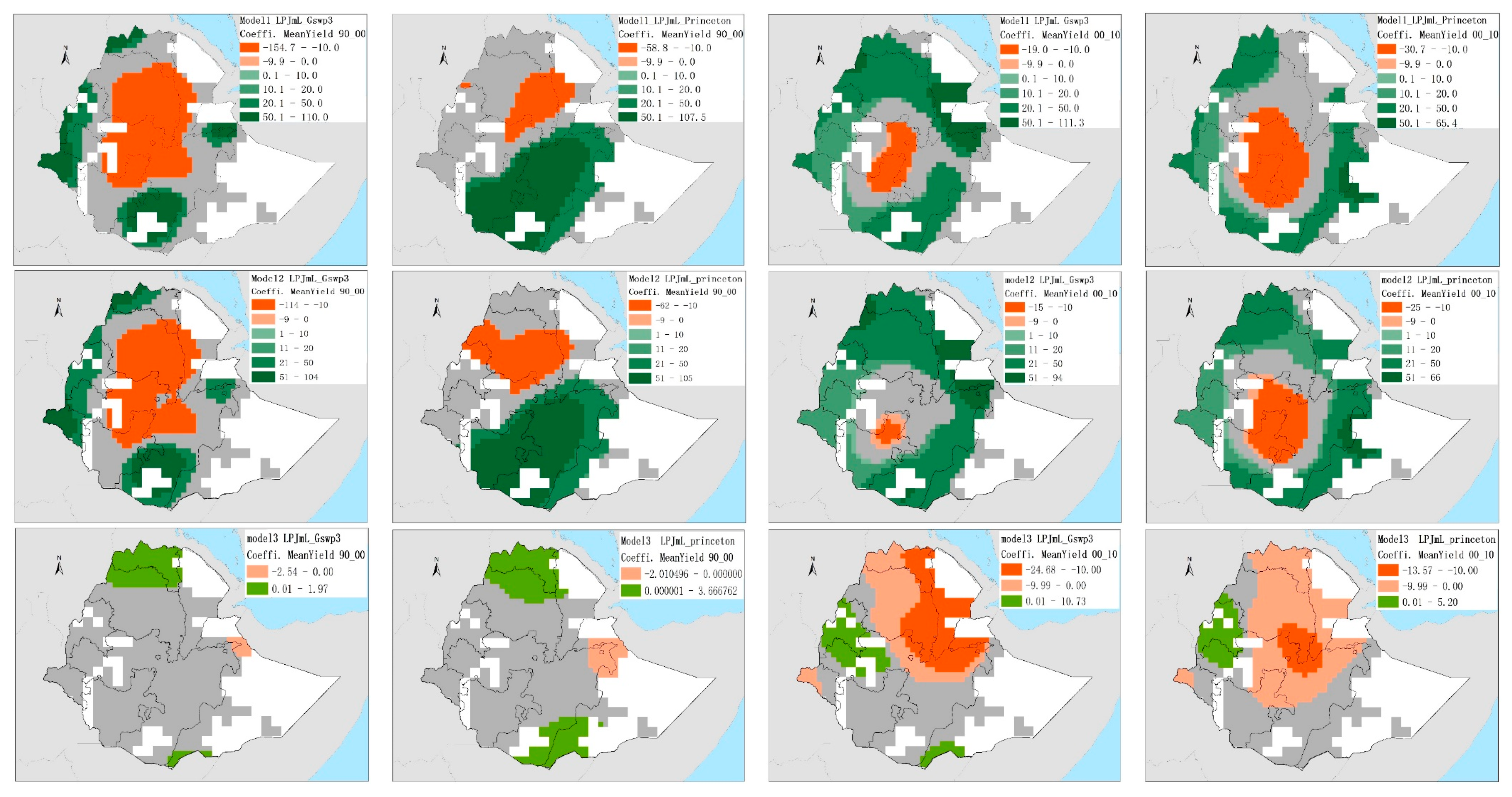
4.3. GWR Results
5. Discussion
6. Conclusions
Author Contributions
Funding
Acknowledgments
Conflicts of Interest
References
- Lee, R. The Outlook for Population Growth. Science 2011, 333, 569–573. [Google Scholar] [CrossRef] [PubMed]
- UN. World Population Prospects: The 2015 Revision, Highlights. Popul. Dev. Rev. 2015, 36, 854–855. [Google Scholar]
- De Sherbinin, A.; Carr, D.; Cassels, S.; Jiang, L. Population and environment. Annu. Rev. Environ. Resour. 2007, 32, 345–373. [Google Scholar] [CrossRef] [PubMed]
- Walker, R.J. Population Growth and its Implications for Global Security. Am. J. Econ. Sociol. 2016, 75, 980–1004. [Google Scholar] [CrossRef]
- Hummel, D.; Adamo, S.; de Sherbinin, A.; Murphy, L.; Aggarwal, R.; Zulu, L.; Liu, J.; Knight, K. Inter- and transdisciplinary approaches to population-environment research for sustainability aims: A review and appraisal. Popul. Environ. 2013, 34, 481–509. [Google Scholar] [CrossRef]
- Bloom, D.E. 7 Billion and Counting. Science 2011, 333, 562–569. [Google Scholar] [CrossRef]
- Wada, Y.; Gleeson, T.; Esnault, L. Wedge approach to water stress. Nat. Geosci. 2014, 7, 615–617. [Google Scholar]
- Geist, H.J.; Lambin, E.F. Proximate causes and underlying driving forces of tropical deforestation. Bioscience 2002, 52, 143–150. [Google Scholar] [CrossRef]
- Godfray, H.C.J.; Beddington, J.R.; Crute, I.R.; Haddad, L.; Lawrence, D.; Muir, J.F.; Pretty, J.; Robinson, S.; Thomas, S.M.; Toulmin, C. Food Security: The Challenge of Feeding 9 Billion People. Science 2010, 327, 812–818. [Google Scholar] [CrossRef]
- Thiede, B.; Gray, C.; Mueller, V. Climate variability and inter-provincial migration in South America, 1970-2011. Glob. Environ. Change-Human Policy Dimens. 2016, 41, 228–240. [Google Scholar] [CrossRef]
- De Sherbinin, A.; VanWey, L.K.; McSweeney, K.; Aggarwal, R.M.; Barbieri, A.; Henry, S.; Hunter, L.M.; Twine, W.; Walker, R. Rural household demographics, livelihoods and the environment. Glob. Environ. Change-Human Policy Dimens. 2008, 18, 38–53. [Google Scholar] [CrossRef] [PubMed]
- Nawrotzki, R.J.; DeWaard, J.; Bakhtsiyarava, M.; Ha, J.T. Climate shocks and rural-urban migration in Mexico: Exploring nonlinearities and thresholds. Clim. Chang 2017, 140, 243–258. [Google Scholar] [CrossRef] [PubMed]
- Gutierrez-Posada, D.; Rubiera-Morollon, F.; Vinuela, A. Heterogeneity in the Determinants of Population Growth at the Local Level: Analysis of the Spanish Case with a GWR Approach. Int. Reg. Sci. Rev. 2017, 40, 211–240. [Google Scholar] [CrossRef]
- Beeson, P.E.; DeJong, D.N.; Troesken, W. Population growth in US counties, 1840–1990. Reg. Sci. Urb. Econ. 2001, 31, 669–699. [Google Scholar] [CrossRef]
- Cervero, R. Road expansion, urban growth, and induced travel-A path analysis. J. Am. Plan. Assoc. 2003, 69, 145–163. [Google Scholar] [CrossRef]
- Lutz, W.; KC, S. Global Human Capital: Integrating Education and Population. Science 2011, 333, 587–592. [Google Scholar] [CrossRef]
- Warner, K. Global environmental change and migration: Governance challenges. Glob. Environ. Chang. Hum. Policy Dimens. 2010, 20, 402–413. [Google Scholar] [CrossRef]
- Arnell, N.W. Climate change and global water resources: SRES emissions and socio-economic scenarios. Glob. Environ. Chang. Hum. Policy Dimens. 2004, 14, 31–52. [Google Scholar] [CrossRef]
- Stephane Hallegatte, M.B.; Laura Bonzanigo, M.F.; Tamaro Kane, U.N.; Julie Rozenberg, D.T.; Vogt-Schilb, A. Shock Waves: Managing the Impacts of Climate Change on Poverty; Climate Change and Development; World Bank: Washington, DC, USA, 2016. [Google Scholar]
- Vorosmarty, C.J.; Green, P.; Salisbury, J.; Lammers, R.B. Global water resources: Vulnerability from climate change and population growth. Science 2000, 289, 284–288. [Google Scholar] [CrossRef]
- Mueller, V.; Gray, C.; Kosec, K. Heat stress increases long-term human migration in rural Pakistan. Nat. Clim. Chang. 2014, 4, 182–185. [Google Scholar] [CrossRef]
- Warner, K. Human migration and displacement in the context of adaptation to climate change: The Cancun Adaptation Framework and potential for future action. Environ. Plan. C Gov. Policy 2012, 30, 1061–1077. [Google Scholar] [CrossRef]
- Hayes, A.C.; Adamo, S.B. Introduction: Understanding the links between population dynamics and climate change. Popul. Environ. 2014, 35, 225–230. [Google Scholar] [CrossRef]
- Chowdhury, A.K.; Kar, K.K.; Shahid, S.; Chowdhury, R.; Rashid, M.M. Evaluation of spatio-temporal rainfall variability and performance of a stochastic rainfall model in Bangladesh. Int. J. Climatol. 2019, 39, 4256–4273. [Google Scholar] [CrossRef]
- McLeman, R.; Smit, B. Migration as an adaptation to climate change. Clim. Chang. 2006, 76, 31–53. [Google Scholar] [CrossRef]
- WorldBank. World Development Indicators. Available online: http://databank.worldbank.org/data/Views/Reports/ReportWidgetCustom.aspx?Report_Name=CountryProfile&Id=b450fd57&tbar=y&dd=y&inf=n&zm=n (accessed on 1 December 2017).
- ILO ILOSTAT 2017. Available online: http://www.ilo.org/global/statistics-and-databases/lang--en/index.htm (accessed on 1 December 2017).
- Kerr, R.A. ADAPTATION TO CLIMATE CHANGE Time to Adapt to a Warming World, but Where’s the Science? Science 2011, 334, 1052–1053. [Google Scholar] [CrossRef]
- Yohe, G.; Tol, R.S.J. Indicators for social and economic coping capacity-moving toward a working definition of adaptive capacity. Glob. Environ. Chang. Hum. Policy Dimens. 2002, 12, 25–40. [Google Scholar] [CrossRef]
- Cai, R.; Feng, S.; Oppenheimer, M.; Pytlikova, M. Climate variability and international migration: The importance of the agricultural linkage. J. Environ. Econ. Manag. 2016, 79 (Suppl. C), 135–151. [Google Scholar] [CrossRef]
- Alcamo, J.; Florke, M.; Marker, M. Future long-term changes in global water resources driven by socio-economic and climatic changes. Hydrol. Sci. J. 2007, 52, 247–275. [Google Scholar] [CrossRef]
- De Sherbinin, A.; Castro, M.; Gemenne, F.; Cernea, M.M.; Adamo, S.; Fearnside, P.M.; Krieger, G.; Lahmani, S.; Oliver-Smith, A.; Pankhurst, A.; et al. Preparing for Resettlement Associated with Climate Change. Science 2011, 334, 456–457. [Google Scholar] [CrossRef]
- CIESIN (Center for International Earth Science Information Network—Columbia University). Gridded Population of the World, Version 4 (GPWv4): Population Count Adjusted to Match 2015 Revision of UN WPP Country Totals; NASA Socioeconomic Data and Applications Center (SEDAC): Palisades, NY, USA, 2016. [CrossRef]
- Doxsey-Whitfield, E.; MacManus, K.; Adamo, S.B.; Pistolesi, L.; Squires, J.; Borkovska, O.; Baptista, S.R. Taking Advantage of the Improved Availability of Census Data: A First Look at the Gridded Population of the World, Version 4. Pap. Appl. Geogr. 2015, 1, 226–234. [Google Scholar] [CrossRef]
- Warszawski, L.; Frieler, K.; Huber, V.; Piontek, F.; Serdeczny, O.; Schewe, J. The Inter-Sectoral Impact Model Intercomparison Project (ISI–MIP): Project framework. Proc. Natl. Acad. Sci. USA 2014, 111, 3228–3232. [Google Scholar] [CrossRef] [PubMed]
- Rosenzweig, C.; Arnell, N.W.; Ebi, K.L.; Lotze-Campen, H.; Raes, F.; Rapley, C.; Smith, M.S.; Cramer, W.; Frieler, K.; Reyer, C.P.O.; et al. Assessing inter-sectoral climate change risks: The role of ISIMIP. Environ. Res. Lett. 2017, 12, 010301. [Google Scholar] [CrossRef] [Green Version]
- Frieler, K.; Lange, S.; Piontek, F.; Reyer, C.P.O.; Schewe, J.; Warszawski, L.; Zhao, F.; Chini, L.; Denvil, S.; Emanuel, K.; et al. Assessing the impacts of 1.5 °C global warming—simulation protocol of the Inter-Sectoral Impact Model Intercomparison Project (ISIMIP2b). Geosci. Model Dev. 2017, 10, 4321–4345. [Google Scholar] [CrossRef] [Green Version]
- Schewe, J.; Gosling, S.N.; Reyer, C.; Zhao, F.; Ciais, P.; Elliott, J.; Francois, L.; Huber, V.; Lotze, H.K.; Seneviratne, S.I.; et al. State-of-the-art global models underestimate impacts from climate extremes. Nat. Commun. 2019, 10, 1005. [Google Scholar] [CrossRef] [Green Version]
- Harper, S. Population-Environment Interactions: European Migration, Population Composition and Climate Change. Environ. Resour. Econ. 2013, 55, 525–541. [Google Scholar] [CrossRef]
- Bondeau, A.; Smith, P.C.; Zaehle, S.; Schaphoff, S.; Lucht, W.; Cramer, W.; Gerten, D.; Lotze-campen, H.; Müller, C.; Reichstein, M.; et al. Modelling the role of agriculture for the 20th century global terrestrial carbon balance. Glob. Change Biol. 2007, 13, 679–706. [Google Scholar] [CrossRef]
- Rost, S.; Gerten, D.; Bondeau, A.; Lucht, W.; Rohwer, J.; Schaphoff, S. Agricultural green and blue water consumption and its influence on the global water system. Water Resour. Res. 2008, 44, 1–17. [Google Scholar] [CrossRef] [Green Version]
- Von Bloh, W.; Schaphoff, S.; Müller, C.; Rolinski, S.; Waha, K.; Zaehle, S. Implementing the nitrogen cycle into the dynamic global vegetation, hydrology, and crop growth model LPJmL (version 5.0). Geosci. Model Dev. 2018, 11, 2789–2812. [Google Scholar] [CrossRef] [Green Version]
- Schaphoff, S.; von Bloh, W.; Rammig, A.; Thonicke, K.; Biemans, H.; Forkel, M.; Gerten, D.; Heinke, J.; Jägermeyr, J.; Knauer, J.; et al. LPJmL4—A dynamic global vegetation model with managed land—Part 1: Model description. Geosci. Model Dev. 2018, 11, 1343–1375. [Google Scholar] [CrossRef] [Green Version]
- Schaphoff, S.; Forkel, M.; Müller, C.; Knauer, J.; von Bloh, W.; Gerten, D.; Jägermeyr, J.; Lucht, W.; Rammig, A.; Thonicke, K.; et al. LPJmL4—A dynamic global vegetation model with managed land—Part 2: Model evaluation. Geosci. Model Dev. 2018, 11, 1377–1403. [Google Scholar] [CrossRef]
- Müller, C.; Elliott, J.; Chryssanthacopoulos, J.; Arneth, A.; Balkovic, J.; Ciais, P.; Deryng, D.; Folberth, C.; Glotter, M.; Hoek, S.; et al. Global gridded crop model evaluation: Benchmarking, skills, deficiencies and implications. Geosci. Model Dev. 2017, 10, 1403–1422. [Google Scholar] [CrossRef] [Green Version]
- Van den Hurk, B.; Kim, H.; Krinner, G.; Seneviratne, S.I.; Derksen, C.; Oki, T.; Douville, H.; Colin, J.; Ducharne, A.; Cheruy, F.; et al. LS3MIP (v1.0) contribution to CMIP6: The Land Surface, Snow and Soil moisture Model Intercomparison Project—Aims, setup and expected outcome. Geosci. Model Dev. 2016, 9, 2809–2832. [Google Scholar] [CrossRef] [Green Version]
- Sheffield, J.; Goteti, G.; Wood, E.F. Development of a 50-Year High-Resolution Global Dataset of Meteorological Forcings for Land Surface Modeling. J. Clim. 2006, 19, 3088–3111. [Google Scholar] [CrossRef] [Green Version]
- Lesk, C.; Rowhani, P.; Ramankutty, N. Influence of extreme weather disasters on global crop production. Nature 2016, 529, 84. [Google Scholar] [CrossRef] [PubMed]
- Easterling, D.R.; Meehl, G.A.; Parmesan, C.; Changnon, S.A.; Karl, T.R.; Mearns, L.O. Climate extremes: Observations, modeling, and impacts. Science 2000, 289, 2068–2074. [Google Scholar] [CrossRef] [Green Version]
- Krishnamurthy, P.K. Disaster-induced migration: Assessing the impact of extreme weather events on livelihoods. Environ. Hazard. Hum. Policy Dimens. 2012, 11, 96–111. [Google Scholar] [CrossRef]
- Piguet, E. From Primitive Migration to Climate Refugees: The Curious Fate of the Natural Environment in Migration Studies. Ann. Assoc. Am. Geogr. 2013, 103, 148–162. [Google Scholar] [CrossRef]
- Hunter, L.M.; Luna, J.K.; Norton, R.M. Environmental Dimensions of Migration. Annu. Rev. Sociol. 2015, 41, 377–397. [Google Scholar] [CrossRef]
- Sibly, R.M.; Hone, J. Population growth rate and its determinants: An overview. Philos. Trans. R. Soc. Lond. Ser. B Biol. Sci. 2002, 357, 1153–1170. [Google Scholar] [CrossRef]
- Ehrlich, P.R.; Holdren, J.P. Impact of Population Growth. Science 1971, 171, 1212–1217. [Google Scholar] [CrossRef]
- Cockx, K.; Canters, F. Incorporating spatial non-stationarity to improve dasymetric mapping of population. Appl. Geogr. 2015, 63, 220–230. [Google Scholar] [CrossRef]
- Xu, Z.; Ouyang, A. The Factors Influencing China’s Population Distribution and Spatial Heterogeneity: A Prefectural-Level Analysis using Geographically Weighted Regression. Appl. Spat. Anal. Policy. 2017, 11. [Google Scholar] [CrossRef]
- Runfola, D.M.; Romero-Lankao, P.; Jiang, L.W.; Hunter, L.M.; Nawrotzki, R.; Sanchez, L. The Influence of Internal Migration on Exposure to Extreme Weather Events in Mexico. Soc. Nat. Resour. 2016, 29, 750–754. [Google Scholar] [CrossRef] [PubMed] [Green Version]
- Cattaneo, C.; Beine, M.; Fröhlich, C.J.; Kniveton, D.; Martinez-Zarzoso, I.; Mastrorillo, M.; Millock, K.; Piguet, E.; Schraven, B. Human Migration in the Era of Climate Change. Rev. Environ. Econ. Policy 2019, 13, 189–206. [Google Scholar] [CrossRef]
- Lonergan, S. The role of environmental degradation in population displacement. Environ. Chang. Secur. Proj. Rep. 1998, 12, 5–15. [Google Scholar]
- Miyan, M.A. Droughts in Asian Least Developed Countries: Vulnerability and sustainability. Weather Clim. Extrem. 2015, 7, 8–23. [Google Scholar] [CrossRef] [Green Version]
- Findley, S.E. Does Drought Increase Migration? A Study of Migration from Rural Mali during the 1983–1985 Drought. Int. Migr. Rev. 1994, 28, 539–553. [Google Scholar]
- Cattaneo, C.; Peri, G. The migration response to increasing temperatures. J. Dev. Econ. 2016, 122, 127–146. [Google Scholar] [CrossRef] [Green Version]
- Black, R.; Bennett, S.R.G.; Thomas, S.M.; Beddington, J.R. Migration as adaptation. Nature 2011, 478, 447–449. [Google Scholar] [CrossRef]


| Category | Variable | Abbreviation | Database | Institution |
|---|---|---|---|---|
| Dependent variable | Population redistribution | PopReDist | GPW 1 | CIESIN 2 |
| Independent variable | Crop yield deviation | MeanYield | ISIMIP 3 | PIK 4 |
| Water flow deviation | MeanFlow | ISIMIP | PIK | |
| Maximum number of consecutive years below median crop yield | ConsecLowYield | ISIMIP | PIK | |
| Maximum number of consecutive years below median water flow | ConsecLowFlow | ISIMIP | PIK | |
| Control Variables | Built-up | Built-up | GHS 5 | EC 6 |
| Population | Pop | GPW | CIESIN |
| Lpjml_Gswp3 | Lpjml_Princeton | |||||||||||
|---|---|---|---|---|---|---|---|---|---|---|---|---|
| Mexico 1990–2000 | PopReDist | MeanYield | MeanFlow | ConsecLowYield | ConsecLowFlow | Built-Up | PopReDist | MeanYield | MeanFlow | ConsecLowYield | ConsecLowFlow | Built-Up |
| MeanYield | 0.167 ** | 0.143 ** | ||||||||||
| MeanFlow | 0.051 ** | 0.168 ** | 0.006 | 0.053 ** | ||||||||
| ConsecLowYield | 0.025 | 0.073 ** | 0.039 * | 0.089 ** | 0.120 ** | −0.102 ** | ||||||
| ConsecLowFlow | −0.024 | −0.006 | −0.054 ** | 0.110 ** | 0.006 | −0.021 | 0.009 | 0.002 | ||||
| Built-up | 0.605 ** | 0.147 ** | 0.042 * | 0.001 | −0.012 | 0.605 ** | 0.137 ** | −0.002 | 0.050 * | 0.027 | ||
| Pop | 0.512 ** | 0.162 ** | 0.033 | 0.026 | −0.008 | 0.859 ** | 0.512 ** | 0.151 ** | −0.008 | 0.060 ** | 0.004 | 0.859 ** |
| Mexico 2000–2010 | PopReDist | MeanYield | MeanFlow | ConsecLowYield | ConsecLowFlow | Built-Up | PopReDist | MeanYield | MeanFlow | ConsecLowYield | ConsecLowFlow | Built-Up |
| MeanYield | 0.142 ** | 0.146 ** | ||||||||||
| MeanFlow | 0.011 | 0.171 ** | 0.038 | 0.223 ** | ||||||||
| ConsecLowYield | −0.036 | −0.180 ** | −0.053 ** | −0.003 | −0.154 ** | −0.072 ** | ||||||
| ConsecLowFlow | 0.028 | −0.046 * | −0.233 ** | 0.075 ** | 0.028 | −0.021 | −0.109 ** | −0.005 | ||||
| Built-up | 0.609 ** | 0.124 ** | 0.009 | −0.028 | 0.033 | 0.609 ** | 0.115 ** | 0.032 | −0.001 | 0.034 | ||
| Pop | 0.454 ** | 0.113 ** | 0.012 | −0.014 | 0.015 | 0.928 ** | 0.454 ** | 0.102 ** | 0.032 * | −0.003 | 0.017 | 0.928 ** |
| Ethiopia 1990–2000 | PopReDist | MeanYield | MeanFlow | ConsecLowYield | ConsecLowFlow | Built-Up | PopReDist | MeanYield | MeanFlow | ConsecLowYield | ConsecLowFlow | Built-Up |
| MeanYield | 0.109 ** | 0.252 ** | ||||||||||
| MeanFlow | 0.163 ** | 0.393 ** | 0.171 ** | 0.566 ** | ||||||||
| ConsecLowYield | −0.002 | 0.043 | 0.089 ** | −0.176 ** | 0.024 | −0.009 | ||||||
| ConsecLowFlow | −0.066 * | 0.029 | 0.249 ** | 0.147 ** | -0.55 | −0.064 * | −0.059 | 0.070 * | ||||
| Built-up | 0.361 ** | 0.003 | 0.072 | 0.009 | −0.012 | 0.361 ** | 0.027 | 0.019 | 0.028 | 0.019 | ||
| Pop | 1.000 ** | 0.109 ** | 0.163 ** | −0.001 | −0.066 ** | 0.363 ** | 1.000 ** | 0.252 ** | 0.172 ** | −0.177 ** | −0.055 | 0.363 ** |
| Ethiopia 2000–2010 | PopReDist | MeanYield | MeanFlow | ConsecLowYield | ConsecLowFlow | Built-Up | PopReDist | MeanYield | MeanFlow | ConsecLowYield | ConsecLowFlow | Built-Up |
| MeanYield | 0.182 ** | 0.100 ** | ||||||||||
| MeanFlow | 0.171 ** | 0.269 ** | 0.080 ** | −0.161 ** | ||||||||
| ConsecLowYield | −0.114 ** | −0.198 ** | −0.152 ** | −0.144 ** | −0.213 ** | −0.114 ** | ||||||
| ConsecLowFlow | −0.077 * | −0.020 | −0.176 ** | 0.187 ** | −0.109 ** | 0.150 ** | −0.155 ** | −0.084 ** | ||||
| Built-up | 0.339 ** | −0.028 | 0.029 | −0.030 | −0.012 | 0.339 ** | −0.050 | 0.043 | −0.043 | 0.014 | ||
| Pop | 0.977 ** | 0.181 ** | 0.186 ** | −0.134 ** | −0.094 ** | 0.391 ** | 0.977 ** | 0.120 ** | 0.048 | −0.133 ** | −0.059 | 0.391 ** |
| 1990–2000 | 2000–2010 | |||||||||||
|---|---|---|---|---|---|---|---|---|---|---|---|---|
| Lpjml_Gswp3 | Model 1 | VIF | Model 2 | VIF | Model 3 | VIF | Model 1 | VIF | Model 2 | VIF | Model 3 | VIF |
| MeanYield | 0.162 *** (0.000) | 1.033 | 0.076 *** (0.000) | 1.055 | 0.082 *** (0.000) | 1.059 | 0.143 *** (0.000) | 1.062 | 0.068 *** (0.000) | 1.078 | 0.091 *** (0.000) | 1.076 |
| MeanFlow | 0.022 (0.273) | 1.033 | 0.011 (0474) | 1.033 | 0.019 (0.259) | 1.033 | −0.006 (0.759) | 1.087 | −0.004 (0.794) | 1.087 | −0.005 (0.782) | 1.087 |
| ConsecLowYield | 0.015 (0.451) | 1.019 | 0.020 (0.199) | 1.019 | 0.007 (0.670) | 1.020 | −0.013 (0.509) | 1.038 | −0.008 (0.623) | 1.038 | −0.016 (0.382) | 1.038 |
| ConsecLowFlow | −0.024 (0.225) | 1.016 | −0.018 (0.248) | 1.016 | −0.019 (0.255) | 1.016 | 0.035 (0.087) | 1.062 | 0.011 (0.482) | 1.063 | 0.026 (0.152) | 1.062 |
| Built-up | 0.593 *** (0.000) | 1.022 | 0.600 *** (0.000) | 1.017 | ||||||||
| Pop | 0.076 *** (0.000) | 1.027 | 0.443 *** (0.000) | 1.013 | ||||||||
| Adjusted R2 | 0.027 | 0.371 | 0.268 | 0.020 | 0.374 | 0.214 | ||||||
| Lpjml_Princeton | Model 1 | VIF | Model 2 | VIF | Model 3 | VIF | Model 1 | VIF | Model 2 | VIF | Model 3 | VIF |
| MeanYield | 0.134 *** (0.000) | 1.020 | 0.054 *** (0.001) | 1.038 | 0.061 *** (0.000) | 1.042 | 0.149 *** (0.000) | 1.078 | 0.080 *** (0.000) | 1.091 | 0.104 *** (0.000) | 1.088 |
| MeanFlow | 0.005 (0.782) | 1.014 | 0.010 (0.523) | 1.014 | 0.012 (0.479) | 1.014 | 0.006 (0.755) | 1.070 | −0.002 (0.918) | 1.070 | 0.001 *** (0.955) | 1.070 |
| ConsecLowYield | 0.074 *** (0.000) | 1.026 | 0.055 *** (0.001) | 1.027 | 0.053 *** (0.002) | 1.028 | 0.021 (0.293) | 1.026 | 0.010 (0.510) | 1.026 | 0.015 (0.410) | 1.026 |
| ConsecLowFlow | 0.008 (0.664) | 1.001 | −0.009 (0.559) | 1.001 | 0.005 (0.773) | 1.001 | 0.032 (0.106) | 1.012 | 0.009 (0.570) | 1.014 | 0.023 (0.193) | 1.013 |
| Built-up | 0.595 *** (0.000) | 1.021 | 0.600 *** (0.000) | 1.015 | ||||||||
| Pop | 0.499 *** (0.000) | 1.025 | 0.443 *** (0.000) | 1.011 | ||||||||
| Adjusted R2 | 0.024 | 0.371 | 0.268 | 0.021 | 0.376 | 0.215 | ||||||
| 1990–2000 | 2000–2010 | |||||||||||
|---|---|---|---|---|---|---|---|---|---|---|---|---|
| Lpjml_Gswp3 | Model 1 | VIF | Model 2 | VIF | Model 3 | VIF | Model 1 | VIF | Model 2 | VIF | Model 3 | VIF |
| MeanYield | 0.173 *** (0.000) | 1.190 | 0.140 *** (0.000) | 1.191 | 0.001 (0.577) | 1.192 | 0.137 *** (0.000) | 1.112 | 0.152 *** (0.000) | 1.114 | 0.010 (0.146) | 1.130 |
| MeanFlow | 0.044 (0.173) | 1.270 | 0.056 * (0.066) | 1.279 | −0.001 (0.732) | 1.301 | 0.117 *** (0.000) | 1.119 | 0.105 *** (0.000) | 1.121 | −0.010 (0.148) | 1.137 |
| ConsecLowYield | −0.003 (0.908) | 1.026 | −0.006(0.828) | 1.026 | −0.001 ** (0.048) | 1.026 | −0.061 ** (0.046) | 1.084 | −0.050 * (0.082) | 1.085 | 0.015 ** (0.024) | 1.091 |
| ConsecLowFlow | −0.110 *** (0.000) | 1.091 | −0.097 *** (0.001) | 1.093 | 0.001 (0.558) | 1.104 | −0.042 (0.170) | 1.064 | −0.042 (0.143) | 1.064 | 0.086 * (0.086) | 1.067 |
| Built-up | 0.350 *** (0.000) | 1.007 | 0.338 *** (0.000) | 1.003 | ||||||||
| Pop | 0.990 *** (0.000) | 1.042 | 0.958 *** (0.000) | 1.068 | ||||||||
| Adjusted R2 | 0.037 | 0.158 | 1.000 | 0.052 | 0.165 | 0.955 | ||||||
| Lpjml_Princeton | Model 1 | Model 2 | Model 3 | Model 1 | Model 2 | Model 3 | ||||||
| MeanYield | 0.235 *** (0.000) | 1.474 | 0.226 *** (0.000) | 1.475 | 0.001 (0.166) | 1.535 | 0.102 ** (0.001) | 1.100 | 0.122 *** (0.000) | 1.103 | −0.010 (0.116) | 1.113 |
| MeanFlow | 0.035 (0.311) | 1.472 | 0.033 (0.307) | 1.472 | −0.001 * (0.075) | 1.474 | 0.063 ** (0.042) | 1.074 | 0.052 * (0.072) | 1.075 | 0.022 ** (0.001) | 1.076 |
| ConsecLowYield | −0.180 *** (0.000) | 1.006 | −0.189 *** (0.000) | 1.007 | 0.001 (0.216) | 1.043 | −0.126 *** (0.000) | 1.079 | −0.109 *** (0.000) | 1.082 | −0.019 ** (0.004) | 1.092 |
| ConsecLowFlow | −0.026 (0.377) | 1.010 | −0.032 (0.227) | 1.010 | −0.001 (0.395) | 1.011 | −0.125 *** (0.000) | 1.048 | −0.133 *** (0.000) | 1.048 | 0.048 *** (0.000) | 1.054 |
| Built-up | 0.360 *** (0.000) | 1.002 | 0.340 *** (0.000) | 1.007 | ||||||||
| Pop | 0.990 *** (0.000) | 1.109 | 0.972 ** (0.000) | 1.036 | ||||||||
| Adjusted R2 | 0.095 | 0.224 | 1.000 | 0.043 | 0.158 | 0.958 | ||||||
© 2019 by the authors. Licensee MDPI, Basel, Switzerland. This article is an open access article distributed under the terms and conditions of the Creative Commons Attribution (CC BY) license (http://creativecommons.org/licenses/by/4.0/).
Share and Cite
Xia, H.; Adamo, S.B.; de Sherbinin, A.; Jones, B. The Influence of Environmental Change (Crops and Water) on Population Redistribution in Mexico and Ethiopia. Appl. Sci. 2019, 9, 5219. https://doi.org/10.3390/app9235219
Xia H, Adamo SB, de Sherbinin A, Jones B. The Influence of Environmental Change (Crops and Water) on Population Redistribution in Mexico and Ethiopia. Applied Sciences. 2019; 9(23):5219. https://doi.org/10.3390/app9235219
Chicago/Turabian StyleXia, Haibin, Susana B. Adamo, Alex de Sherbinin, and Bryan Jones. 2019. "The Influence of Environmental Change (Crops and Water) on Population Redistribution in Mexico and Ethiopia" Applied Sciences 9, no. 23: 5219. https://doi.org/10.3390/app9235219