Article

Optimal Charging of Plug-In Electric Vehicle: Considering Travel Behavior Uncertainties and Battery Degradation

by
Hanif Tayarani
1,
Hamidreza Jahangir
1,
Razieh Nadafianshahamabadi
2,
Masoud Aliakbar Golkar
1,
Ali Ahmadian
3,4,* and
Ali Elkamel
4,5
1
Department of Electrical Engineering, K. N. Toosi University of Technology, Tehran 1969764499, Iran
2
Atkinson Center for a Sustainable Future, Cornell University-Environmental Defense Fund, Ithaca, NY 14853, USA
3
Department of Electrical Engineering, University of Bonab, Bonab 5551761167, Iran
4
College of Engineering, University of Waterloo, Waterloo, ON N2L3G1, Canada
5
College of Engineering, Khalifa University of Science and Technology, The Petroleum Institute, Abu Dhabi 127788, UAE
*
Author to whom correspondence should be addressed.
Appl. Sci. 2019, 9(16), 3420; https://doi.org/10.3390/app9163420
Submission received: 17 July 2019 / Revised: 14 August 2019 / Accepted: 15 August 2019 / Published: 19 August 2019
(This article belongs to the Special Issue Hybrid Vehicle Technologies for a Sustainable Future Mobility)

Abstract

:

Featured Application

Authors are encouraged to provide a concise description of the specific application or a potential application of the work.

Abstract

The negative environmental impacts of using fossil fuel-powered vehicles underlined the need for inventing an alternative eco-friendly transportation fleet. Plug-in electrical vehicles (PEVs) are introduced to cut the continuing increase in energy use and carbon emission of the urban mobility. However, the increased demand for mobility, and therefore energy, can create constraints on the power network which can reduce the benefits of electrification as a certain and reliable source. Thus, the rise in the use of electric vehicles needs electric grids to be able to feed the increased energy demand while the current infrastructure supports it. In this paper, we introduce a methodological framework for scheduling smart PEVs charging by considering the uncertainties and battery degradation. This framework includes an economic model for charging and discharging of PEVs which has been implemented in a 21-node sample distribution network with a wind turbine as a distributed generation (DG) unit. Our proposed approach indicates that the optimal charging of the PEVs has a high impact on the distribution network operation, particularly under the high market penetration of PEVs. Thus, the smart grid to vehicle (G2V) charging mode is a potential solution to maximize the PEV’s owner profit, while considering the battery degradation cost of the PEVs. The simulation result indicates that smart charging effectuation is economical.

1. Introduction

The rapid growth in urban mobility and the corresponding increase in energy use, greenhouse gas emissions, (GHG), air quality [1], and their externalities have driven more people to switch from their conventional cars to cleaner fleets, electric cars. The population of plug-in electric vehicles (PEVs) increased drastically over the past decade [2]. The PEVs are equipped with a large battery bank and the need for fast charging of these batteries and range anxiety issues impose an enormous load demand on the residential and distribution networks and this made many operation problems for the distribution system operator.
Two approaches might be considered when the charging infrastructure is needed. First is developing a charging infrastructure and increasing the capacity of the network which requires further investment in grid peak capacity. The second approach is managing the demand by considering the driving behaviors and charging schedules for cars and predicting the load pattern that the PEVs force on a daily basis. In this approach, if the pricing and rate structure are correctly planned, the demand for additional peak capacity investment will be declined and the cost of PEVs charging will be reduced, in one hand. It also improves the stability of the grid, on the other hand. Grid-to-vehicle (G2V), and vehicle-to-grid (V2G) are the two solutions suggested to avoid the loss of the power grid by supplying the network demand in a peak load period. G2V is the common type of PEV charging procedure, where power goes from grid to vehicle, but V2G, which has various applications in the power system auxiliary services, transfers power from vehicle to grid. In G2V and V2G, the aggregator can control and operate a group of PEVs and these vehicles act like storage systems.
There is a body of literature that proposed various managed PEV charging methods [3,4,5,6,7]. Prior studies in the area of PEVs and electric grid are based on the models, since the actual data of PEVs in a large scale are limited. However, the results of some of the studies are hampered because of much uncertainty surrounding the drivers’ behaviors. For example, the current trend in the literature is to use a simplified PEV travel profile by mapping the travel behavior of conventional vehicles, which might introduce bias into the results. In addition, considering only a single PEV fleet in the simulation as a proof of concept or assuming that all vehicles have the same features are other shortcomings of prior studies [8,9,10,11,12]. The limitations of the distribution network are essential to be considered in the modeling framework, while they are neglected in some prior studies [13,14,15]. On-peak charging might cause serious problems such as voltage instability, reserve capacity, and voltage collapse, voltage insecurity, and power loss. In addition, while dynamic electricity price is critical in a smart charging system, the availability of accurate electricity price is an area of concern in a realistic optimization problem [16,17,18]. Dynamic pricing can encourage PEV owners to charge their vehicles at a lower rate.
In this study, we compare the uncoordinated, smart G2V versus V2G charging mode for a set of PEV fleets in a sample distribution network to understand which charging mode has supremacy over the others. We integrated wind energy into the power grid to consider using renewable energy resources in the grid. To fill the existing gap in the literature, the uncertainties of load, wind speed, electricity price, and travel behavior are studied in the PEV-grid model. A detailed driving pattern including the arrival and departure time and travel distance of PEVs drivers are taken into account. The Monte Carlo simulation with scenario reduction task is also conducted to model the stochastic nature of PEVs’ travel behavior. The probabilistic economic dispatch is also applied to optimize the charging/discharging problem. This study provides insight into the effect of battery degradation in various charging modes (V2G and G2V) and presents the results in an economic and technical view.
The paper is structured as follows: Section 2 includes the problem statement and the method. In Section 3, the numerical results of this study are given in different approaches, which clarify the performance of the proposed method. Section 4 provides the numerical results of different charging procedures. Finally, Section 5 concludes the findings of this study.

2. Problem Statement

In this research, the objective function in the optimization of PEVs smart charging and discharging is to minimize the cost function subject to the network constraint:
s = 1 10 t = 1 24 { [ O C a s ( t ) × R a s ( t ) + O C r s ( t ) × R r s ( t ) + D E C s ( t ) ] } × P r ( s )
where R a s ( t ) is the active and R r s ( t ) is the reactive part of the power supplied in the scenario s at time t. Indices s and t are presenting scenario number and time respectively, where s ranges from 1 to 10 to consider all 10 scenarios in this study, and t ranges from 1 to 24, to include all hours in a single day.
O C a s ( t ) and O C r s ( t ) are the price for active and reactive power, and D E C s ( t ) is PEVs fleet total battery degradation cost in the scenario s, respectively. The probability of each scenario is presented by P r ( s ) . The load and generation equation can be written as follows [16]:
s 10 t 24 R a s ( t ) + s 10 t 24 W a s ( t ) = s 10 t 24 L a s ( t ) + s 10 t 24 P E V a s ( t ) + s 10 t 24 P l o s s a s ( t )
s 10 t 24 R r s ( t ) + s 10 t 24 W r s ( t ) = s 10 t 24 L r s ( t ) + s 10 t 24 P E V r s ( t ) + s 10 t 24 P l o s s r s ( t )
where W a s ( t ) is the active power that the wind turbines produce, L a s ( t ) is the real part of load demand, and P E V a s ( t ) is the absorbed or injected active power by PEVs in time t and scenario s. W r s ( t ) is the reactive power produced by the wind turbines, L r s ( t ) is the reactive part of the demand and P E V r s ( t ) is the absorbed reactive power that is consumed by the charging equipment.
P l o s s a s ( t ) and P l o s s r s ( t ) are power loss in a transmission line that can be calculated using Equations (4) and (5) [19]:
P l o s s a s ( t ) = i = 1 n V s ( i , j , t ) × j = 1 n V s ( i , j , t ) × { G ( i , j ) × cos ( θ s , i , t θ s , j , t ) + B ( i , j ) × sin ( θ s , i , t θ s , j , t ) }
P l o s s r s ( t ) = i = 1 n V s ( i , j , t ) × j = 1 n V s ( i , j , t ) × { G ( i , j ) × cos ( θ s , i , t θ s , j , t ) B ( i , j ) × sin ( θ s , i , t θ s , j , t ) }
where i and j are indices of buses and n is the number of buses. G and B are the real and imaginary part of the admittance matrix, and θ is the voltage angle in this equation. V s ( i , j , t ) is the voltage difference between buses i and j at time t in scenario s.
In this framework, power and constraint of all nodes such as a voltage of nodes and frequency of system should not surpass the boundaries limitation. The nodes’ constraints are introduced in Equations (6) and (7) [20].
P u ( t ) P max u ,   Q u ( t ) Q max u u = 1 , 2 , , n e q ,   n e q = t o t a l   n u m b e r   o f   b u s e s
V min V l ( t ) V max ,   l = 1 , 2 , , n L D   t = 1 , 2 , , 24    n L D = t o t a l   n u m b e r   o f   l o a d   n o d e s
P u ( t ) and Q u ( t ) represent active and reactive consumed power by the equipment u, which must not pass the equipment’s maximum active and reactive power that are presented by P max u and Q max u . Voltage magnitude of all nodes V l ( t ) must stay between the minimum and maximum value of them, which are presented by V min , V max . The most significant restraint in PEVs charging and discharging problem is the state of charge (SOC) of the batteries which should fulfill the minimum boundaries at the moment of departure. This constraint is presented in Equation (8) [19]:
S O C p , s ( t d e p ) S O C d e p    p = 1 , 2 , , N P E V    N P E V = t o t a l   n u m b e r   o f   P E V s
In this study, for customers convenience, it is assumed that the S O C d e p is at least 80 percent of the total capacity [19]. Here, S O C p , s ( t d e p ) shows SOC of p-th PEV battery at the departure time ( t d e p ) in scenario s. The undermentioned constraint must be satisfied for all PEVs’ battery.
S O C p , s ( t ) = S O C p , s ( t 1 ) + P p c h r ( t ) × η c h r P p d i c h r ( t ) / η d i c h r p = 1 , 2 , , N P E V    t = 1 , 2 , , 24
where, P p c h r ( t ) , P p d i c h r ( t ) are charging and discharging rate of each PEVs in time interval t, and η c h r , η d i c h r are the total efficiency of battery charging/discharging and converter, respectively [16].
In Equation (10), battery degradation cost has been calculated based on the PEVs total battery degradation at each time for each scenario [21].
D E C s = s = 1 10 ( p = 1 N P E V   c = 1 n p c y c [ C p B a t t × D p , s T O T × T c , s c y c Q p 0 Q p U s e ] ) T c c y c = c - t h   C h a r g i n g   c y c l e
where C p B a t t is the p-th PEV battery cost and D p , s T O T represents summation of calendar ( D p , s C A L ) and cyclic ( D p , s C Y C ) degradation of PEVs’ battery in the cycle of T c , s c y c in scenario s and cycle c. Also, Q p 0 , Q p U s e stand for the nominal and useful capacity of p-th PEV, respectively. Q p U s e is extracted based on Equation (11).
Q p U S E = ρ × Q p 0    0 < ρ < 1
Stem from the United States Advanced Battery Consortium (USABC) PEVs’ battery should be changed if the battery capacity is reduced to 80% of its total capacity [21], thus ρ = 0.8 .
D p , s T O T ( T c , s c y c ) = D p , s C A L ( T c , s c y c ) + D p , s C Y C ( T c , s c y c )
Equations (13) and (14) illustrate the mechanism of the calculating calendar ( D p , s C A L ) and cyclic ( D p , s C Y C ) degradation [21].
D p , s C A L ( T c , s c y c ) = Q p 0 × exp ( S O C p , s ( T c , s c y c ) S O C ¯ b ) × exp ( ψ B ψ 0 a ) × t s
D p , s C Y C ( T c , s c y c ) = α 1 × [ D O D p , s ( T c , s c y c ) ] 2 + α 2 × D O D p , s ( T c , s c y c ) + α 3
To model the degradation of the PEVs’ batteries, two main criteria including calendar degradation ( D p , s C A L ) and cycling degradation are considered. Employing calendar degradation ( D p , s C A L ), which is a function of the SOC of p-th PEV over period T ( S O C p , s ( T c , s c y c ) ), nominal SOC of p-th PEV ( S O C ¯ ), ambient temperature ( ψ B ), nominal temperature ( ψ 0 ), and charging time ( t s ), is a vital part in battery degradation task. Also, a and b are calendar degradation’s fitting parameter. The cycling degradation, which is a function of DOD over period T ( D O D p , s ( T c , s c y c ) ), has a significant effect on the total battery life. a and b in Equation (13) are fitting parameters for calendar degradation. α 1 , α 2 , and α 3 are fitting parameters for cycling degradation related to DOD. In Equation (15), the benefits of PEV aggregator has been introduced.
P E V s   b e n e f i t = s = 1 10 t = 1 24 p = 1 n p e v { O C a s ( t ) × P r ( s ) × [ P E V a s ( t ) | m = U N C P E V a s ( t ) | m = s m a r t ] } + s = 1 10 t = 1 24 p = 1 n p e v { O C r s ( t ) × P r ( s ) × [ P E V r s ( t ) | m = U N C P E V r s ( t ) | m = s m a r t ] }
where the welfare is calculated as the difference between power consumed by charging and discharging of PEVs’ batteries in two charging modes: uncoordinated and smart charging [21].
The power loss in the transmission line in the smart charging mode is different from the uncoordinated mode, and the difference between this two is considered as the network benefit.
N e t w o r k   b e n e f i t = s = 1 10 t = 1 24 p = 1 n p e v { O C a s ( t ) × P r ( s ) × [ P l o s s a s ( t ) | m = U N C P l o s s a s ( t ) | m = s m a r t ] } + s = 1 10 t = 1 24 p = 1 n p e v { O C r s ( t ) × P r ( s ) × [ P l o s s r s ( t ) | m = U N C P l o s s r s ( t ) | m = s m a r t ] }
The total benefit of using smart charging and discharging of PEV batteries in smart G2V and V2G mode is calculated using Equation (17).
N e t   p r o f i t = [ P E V s   b e n e f i t + N e t w o r k   b e n e f i t ] C inf
where the C inf is installing smart charging and equipment cost that is extracted from [16].

2.1. Methodology

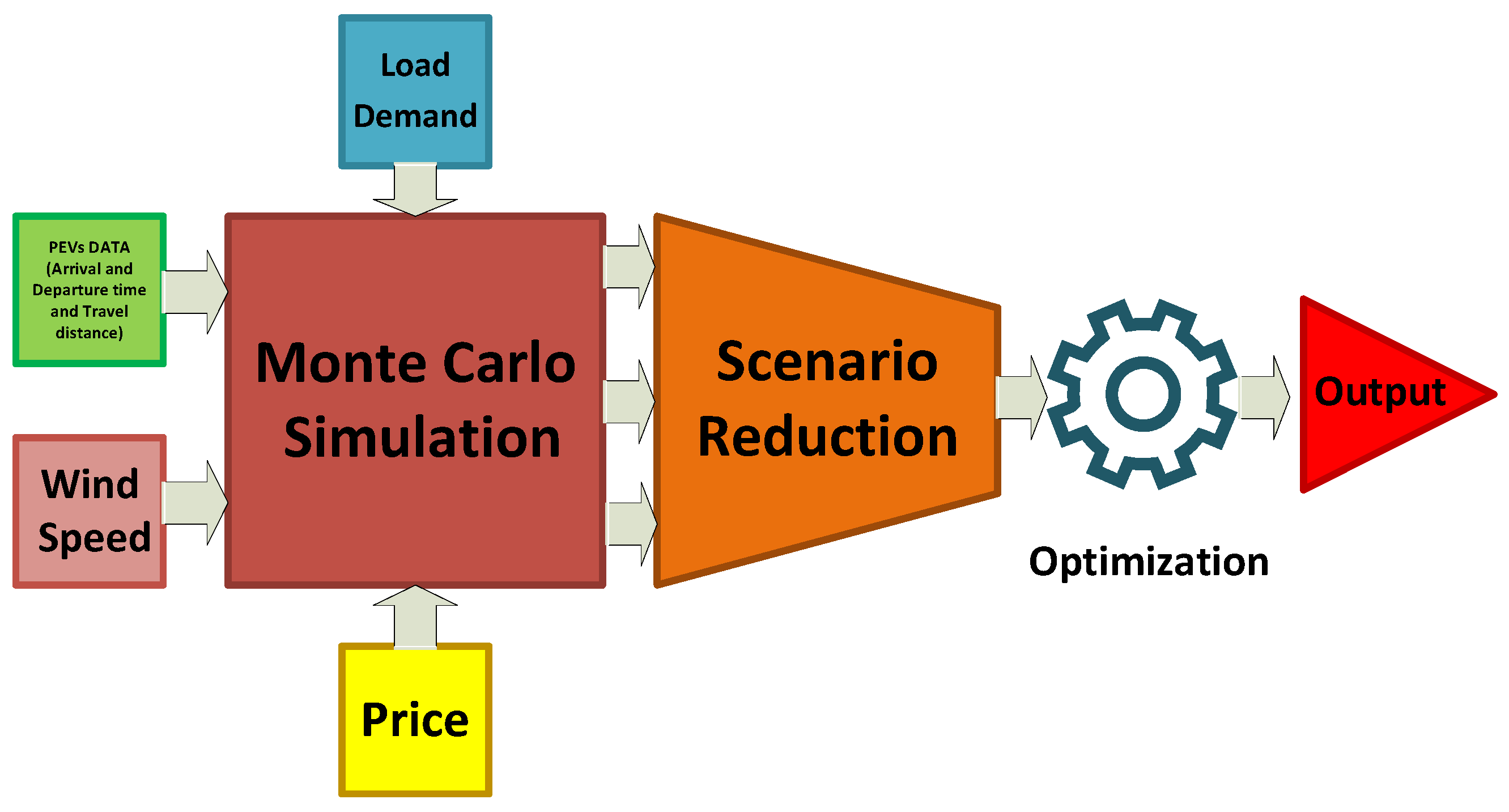
Figure 1 shows the methodological framework of the study. In general, the driving pattern of PEVs drivers, the effects of wind energy, electricity price, and load demand are considered in the simulation. Then the probabilistic economic dispatch is applied to optimize the charging/discharging problem.

2.1.1. Modeling PEVs as Uncertain Enormous Storage

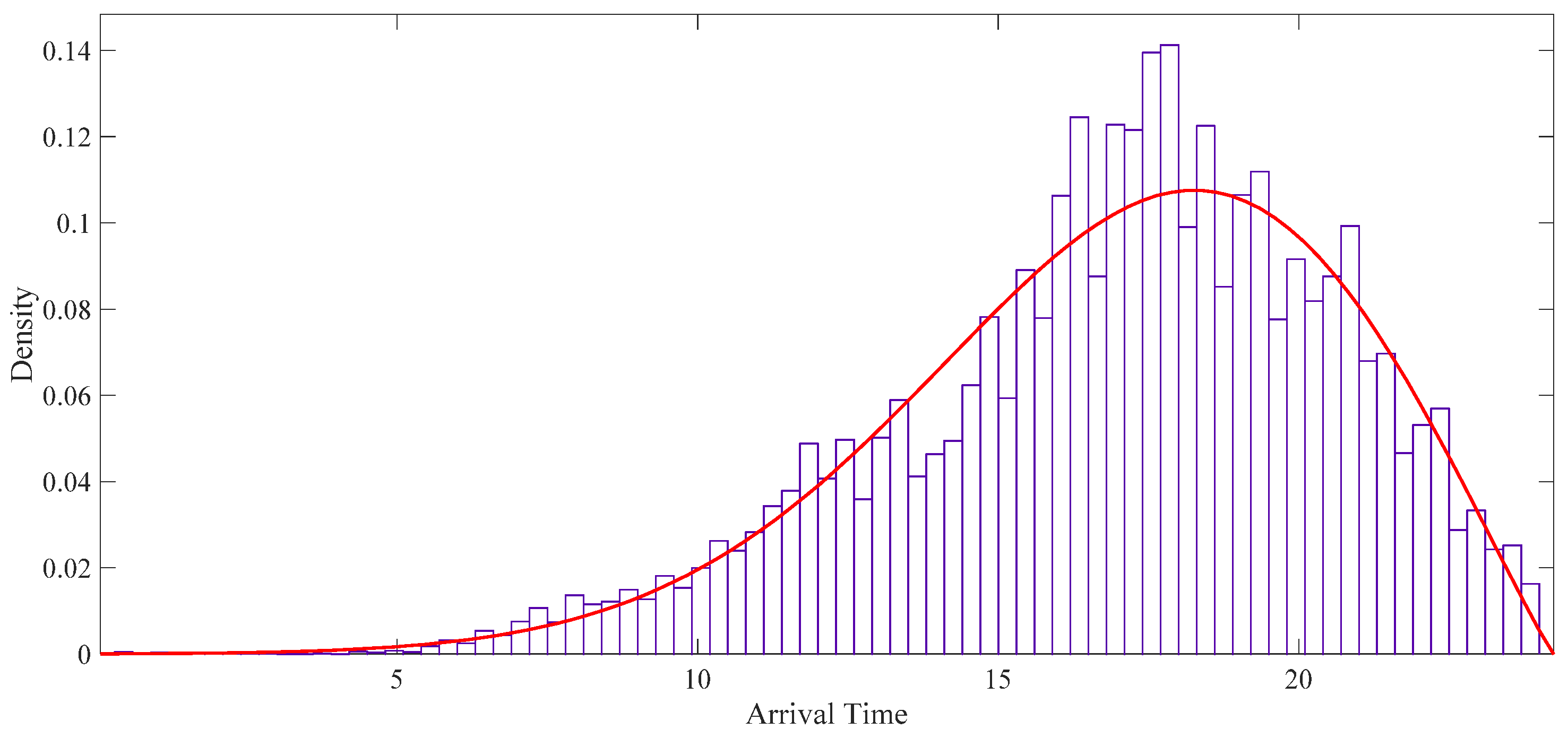
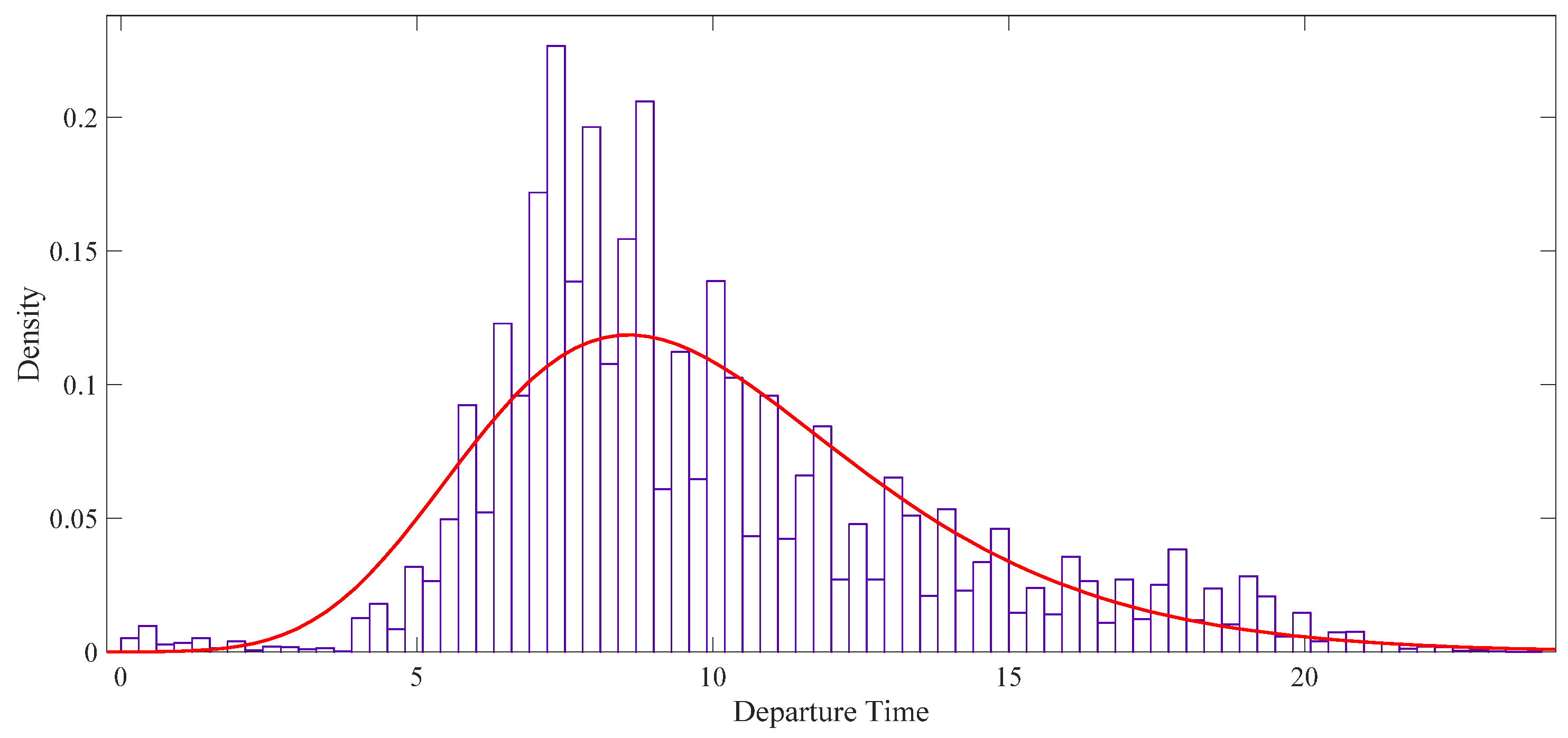
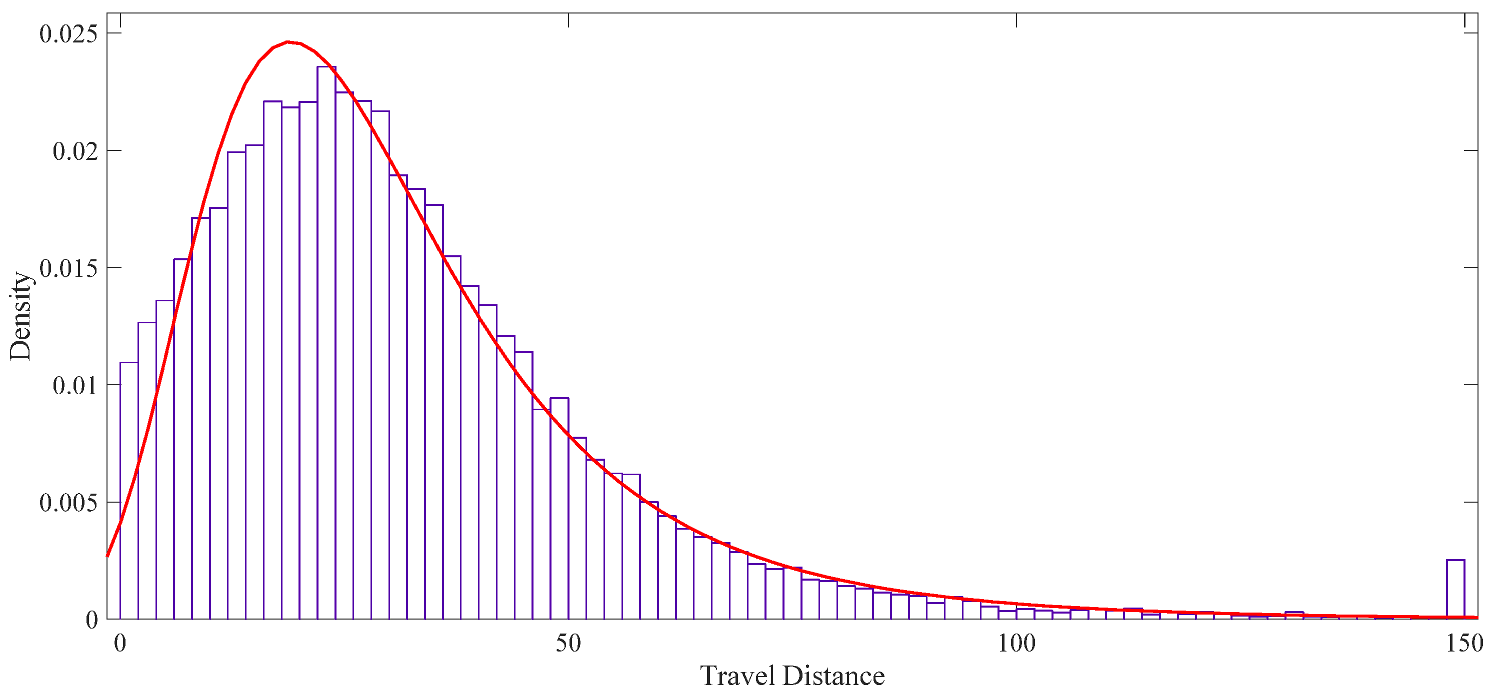
Travel behavior parameters such as arrival and departure times, travel distances, and vehicle type are obtained from the 2017 National Household Travel Survey (NHTS) database. The characteristics of the users are extracted among 23,514 daily trips. Figure 2, Figure 3 and Figure 4 show the probability distribution function (PDF) of arrival time, PDF of departure time, and PDF of travel distance.
It is important to specify the initial amount of PEVs’ SOCs. Monte-Carlo approach is conducted to model the PEVs’ travel behaviors under uncertainties [22]. Monte-Carlo is applied to produce different scenarios based on the input variables such as arrival and departure time, initial SOCs derived from travel distance, and the type of vehicle in order to get battery characteristics. The initial SOC of each PEVs is derived from Equation (18).
S O C i n i t , p n = 100 d p q C e f f × C a p b a t , p × 100
where, d p n is the traveled distance of p-th PEV in q-th iteration by Monte-Carlo simulation, C e f f (km/kWh) presents the efficiency coefficient of the battery during the driving mode, and C a p b a t , p (kWh) is the capacity of p-th PEV’s battery. The parameters of this equation are selected according to the PEVs model. C e f f and C a p b a t , p are obtained from [16,19,23]. The input data are extracted from the probability distribution function (PDF) of travel data to produce the necessary information for PEVs fleet. The distribution function is used to create the PDF of arrival time and travel distance is the generalized extreme value (GEV) distribution which are shown in Figure 2, Figure 3 and Figure 4. Also, for departure time Weibull distribution function is taken into account as shown in Figure 3.

2.1.2. Modeling Load Demand, Price, and Wind Speed Uncertainties

The uncertainties in the load demand, electricity price, and wind speed are simulated by using a Monte-Carlo simulation which produces 1000 scenarios of possible probabilities [24]. The normal and Weibull distribution functions are suitable solutions for modeling system objective uncertainties [25].
The input data for the Monte-Carlo simulation is extracted from the PDF created by normal distribution function for the load demand and electricity price. The PDF created by the Weibull distribution function for the wind speed is also extracted for the Monte-Carlo simulation [24]. Normal and Weibull distribution functions are presented in Equations (19) and (20).
f ( x | μ , σ 2 ) = 1 2 π σ 2 e ( x μ ) 2 2 σ 2
f ( x | λ , κ ) = { κ λ ( κ λ ) κ 1 e ( x λ ) κ x 0 0 x < 0
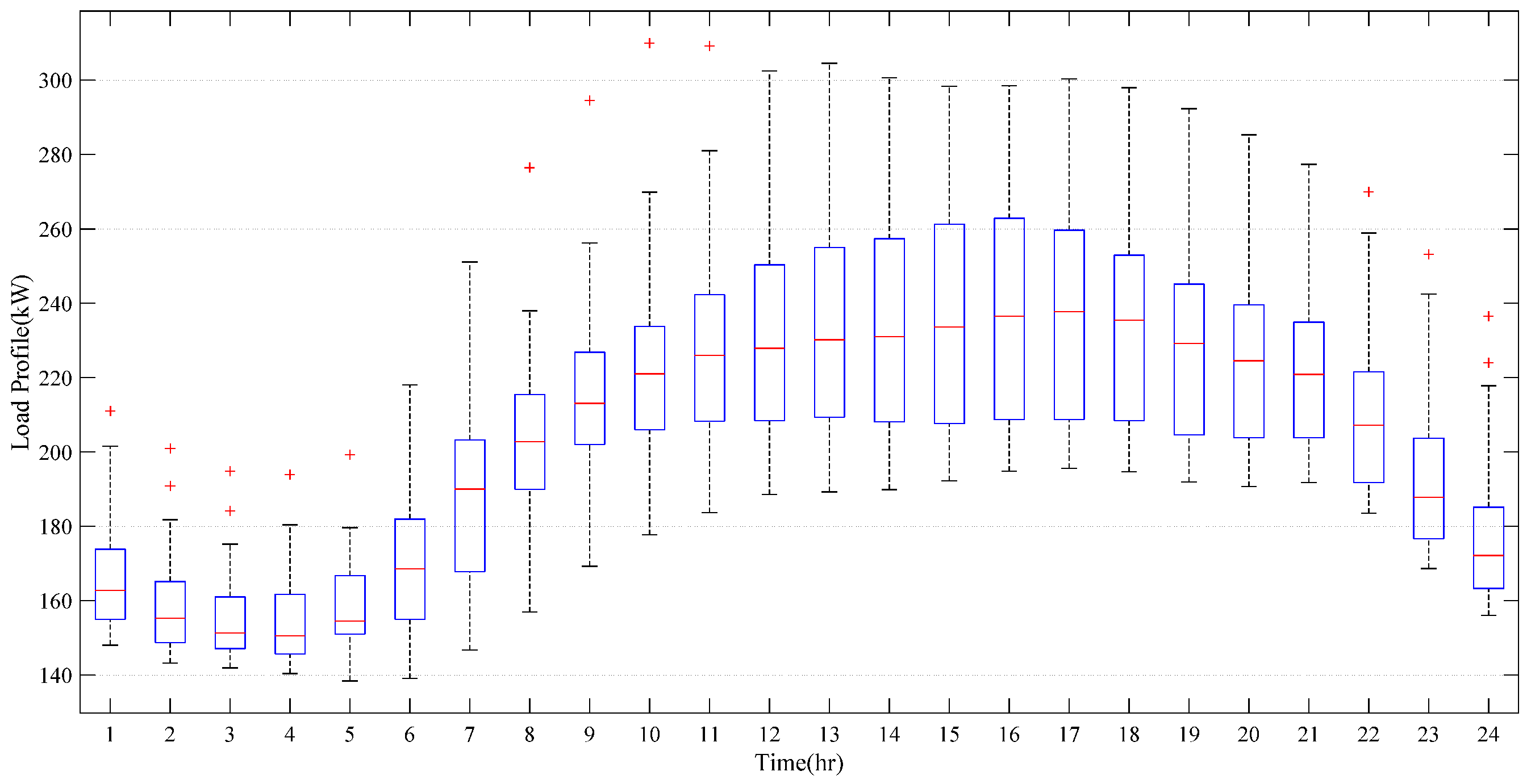
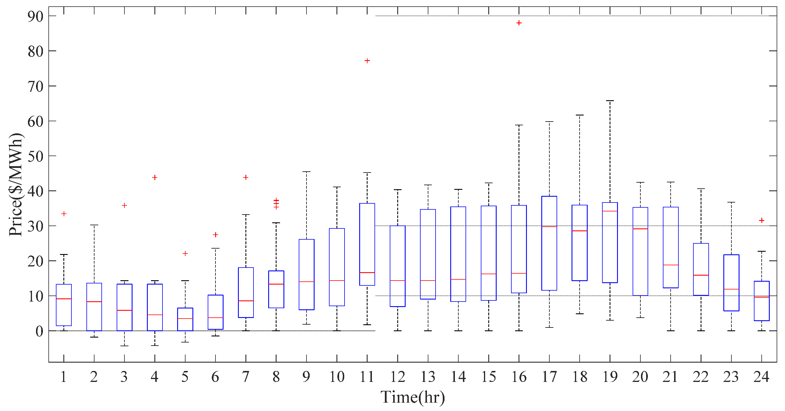
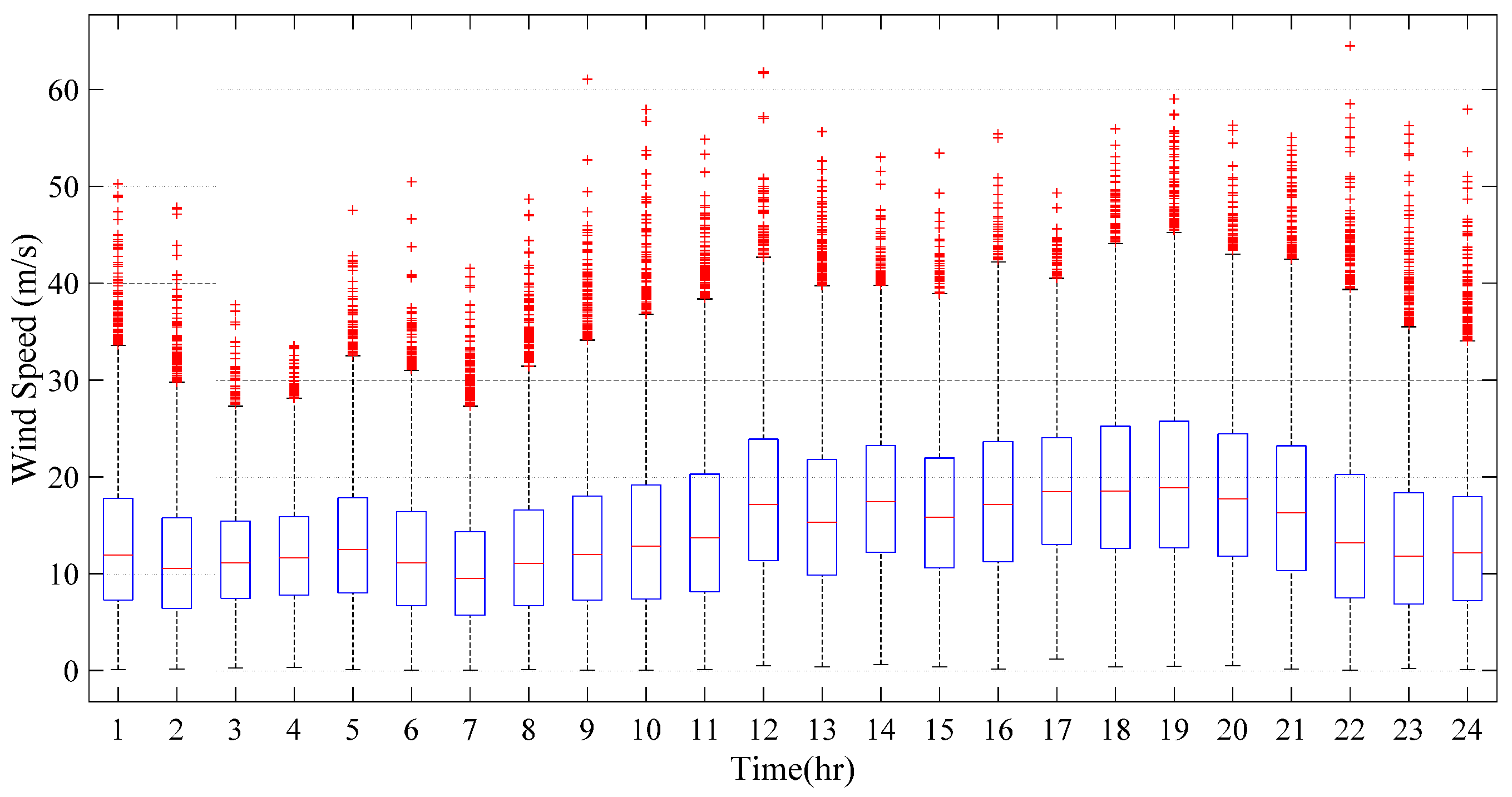
The generated scenarios for load demand, price, and wind are shown in Figure 5, Figure 6 and Figure 7, respectively. The relationship between wind speed and wind power is derived from [26] which is shown in Equation (21). This function transforms the wind speed to electricity power for a wind turbine.
P n w , t w d = { 0 v t < v c i , v t > v c o P W max v r < v t < v c o P W max ( v t v c i ) v r v c i v c i < v t < v r
where P n w , t w d is the power generated by the wind turbine. In general, generated power equals to zero when the wind speed is lower than the cut-in speed ( v c i ) or is greater than the cut-out speed ( v c o ). When the wind speed is between rated and cut-out speed, the turbine produces its nominal power; also if it is between a cut-in and rated speed ( v r ), the generated power is calculated by related function that is shown in Equation (21). Table 1 shows the parameters of the distribution functions for the arrival and departure time and travel distance.

2.1.3. Scenario Reduction

To handle the uncertainty of various stochastic parameters such as electricity price, wind speed, and load demand, the Monte-Carlo simulation task is employed in this study. Monte-Carlo simulation generates various scenarios based on the probability distribution functions. In this study, to increase the accuracy of the forecasting results, 1000 scenarios are generated in the first step. This large volume of data makes high computation cost because calculating economic dispatch for all 1000 scenarios is time-consuming. To handle this problem a scenario reduction task is employed based on the forwarding scenario selection and the backward scenario reduction approaches that are elaborated in [20]. This method eliminates the similar scenarios to 10 final scenarios which have the most probability. This procedure is applied for handling the system uncertainties. For PEV’s modeling, 1000 scenarios which are generated by the Monte-Carlo simulation are reduced to 420 scenarios where 30 PEVs are considered in each bus in distribution network. Then, the economic dispatch is calculated for these scenarios and the vehicle owners’ savings are derived by multiplying the optimized cost function by their relative probability.
The boxplot in Figure 5 shows the load profile of the modeling scenarios after the scenario reduction. Each whisker shows the variability of the load profile of scenarios for each hour of the day. On average, the load profile is higher between 12 pm to 5 pm. Electricity price is at the highest point at 5 pm, when the load profile is also the highest, on average, as shown in Figure 6. Figure 7 shows the scenarios for six wind turbines which generate active and reactive power in the distribution network.

2.1.4. Optimization Procedure

A mixed-integer non-linear problem (MINLP) is presented to optimize the cost function by considering the PEVs batteries’ SOC at the departure time as the optimization constraints. MINLP is considered because of the complexity of the economic dispatch, power loss considerations and network constraints compounded with the charging and discharging of PEVs’ batteries. The main goal is to minimize the Equation (1) by considering the other mentioned constraints such as SOC values.
In the optimization procedure, the maximum value of the PEV’s SOC is not considered as a constraint for the problem formulation. The minimum value of batteries’ SOC is employed as a constraint, so the operator can charge the batteries as much as possible if this procedure is beneficial (i.e., depends on the electricity price and power system load). For solving the MINLP problem, General Algebraic Modelling System (GAMS) software has been used [27]. The “Conopt-4” solver is employed which has the capability to solve the convex nonlinear problem.

3. Results

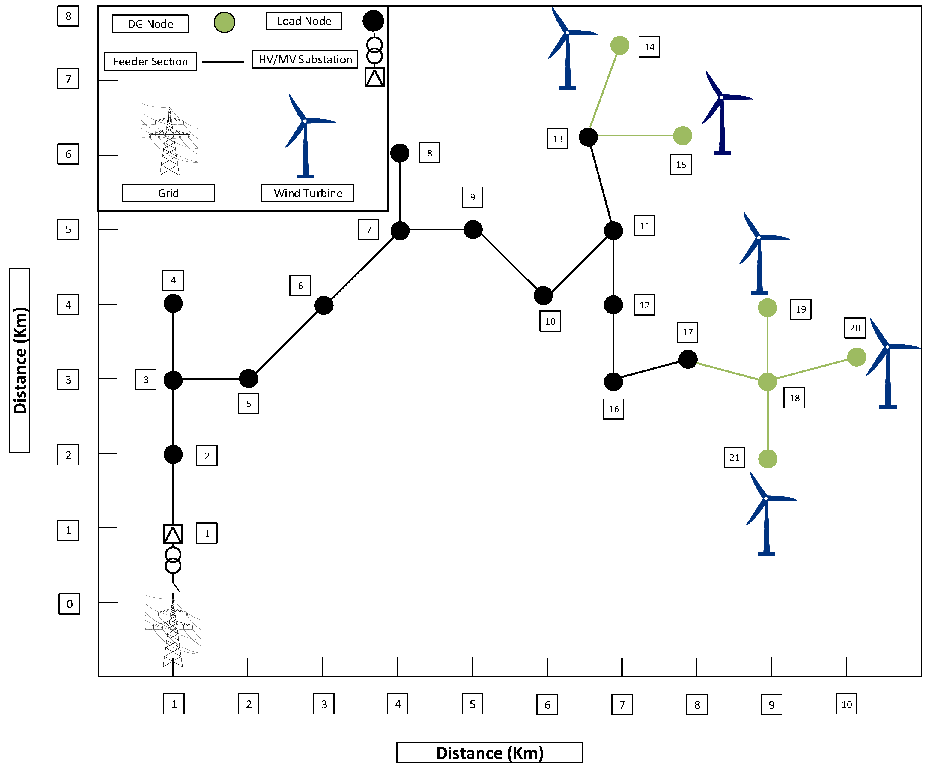
For the numerical study, a 21-node sample distribution network has been employed which is 13.8 Kv and has 20 feeder section which is shown in Figure 8. In this sample, six wind turbines which are able to produce 500 kVA are set up in buses 14, 15, and 18 to 21. The network characteristics and constraints such as voltage deviation and HV/MV substation capacity are derived from [16]. The load demand, electricity price, and wind speed data are simulated by the Monte-Carlo simulation. The normal distribution function for the load demand and electricity price and the Weibull distribution function for the wind speed data are taken into account. The load, electricity price, and wind speed data are for Ontario, Canada [28]. The parameters of the sample network are shown in Table 2. It is assumed that 30 PEVs are connected to each demand node. The information on arrival and departure time, travel distances, and type of vehicles are based on the NHTS database [29]. To show the performance of the proposed charging method, three different approaches including uncoordinated, smart G2V, and smart V2G are considered.

3.1. Uncoordinated Charging

In the uncoordinated charging approach, PEVs drivers plug in their vehicle as soon as they arrive home. The cost of charging is equal to the summation of the consumed power by the PEVs battery to charge the vehicle. There is a considerable peak in the total load demand of charging PEVs because the residual load demand and PEVs load demand occur semi simultaneously. This peak intensifies the importance of using smart charging during a day. In uncoordinated charging during the night, PEVs charging rate is close to zero. The costs and power loss of the uncoordinated charging approach are shown in Table 3.

3.2. Smart G2V Charging

In the G2V approach of charging PEVs, the aggregator can control the rate of power and time of charging. In this way, the amount of money that PEV owners should pay is much lower than the uncoordinated charging modes since the cars can be charged at the off-peak time. Electricity price is negative in several hours a day in Ontario, so it is beneficial for PEVs owners and operators to charge the PEVs at this time. PEV owners will be paid by the network operator due to generation constraints. As 
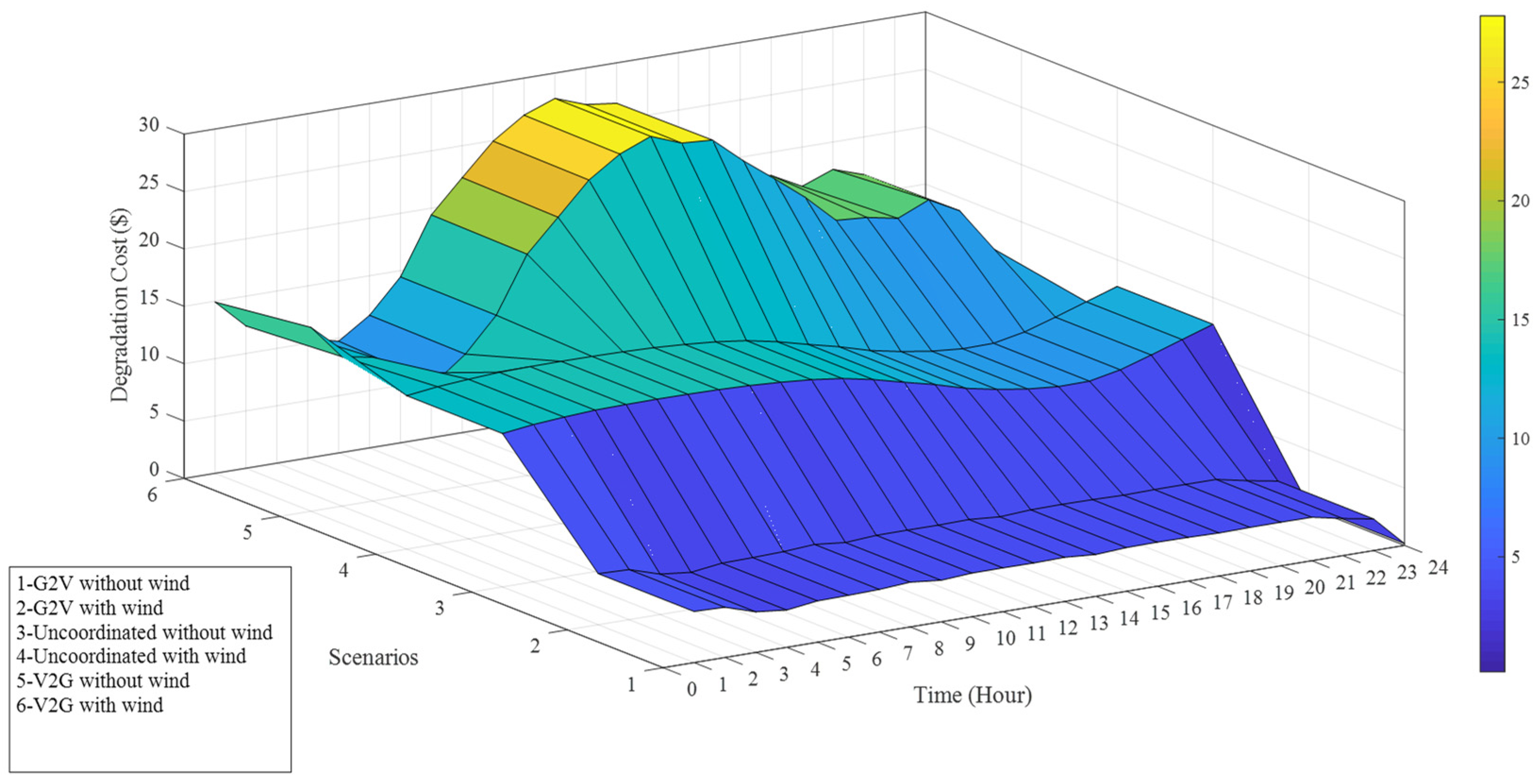
Table 4 shows, purchased energy cost in the smart G2V mode is lower than the uncoordinated charging mode, likewise the degradation cost. The reduction in degradation cost is caused by spreading the charging time interval.

3.3. Smart V2G Charging

In smart V2G charging, the PEVs can operate in both vehicles to the grid (V2G) and grid to vehicle (G2V) modes. The charging rate in every hour is varied to minimize the operation cost and maximize the SOCs of the PEVs. The results are illustrated in Table 5. At this point, the same as G2V charging mode, the purchased energy cost is reduced in comparison with the uncoordinated and smart G2V charging mode. Degradation cost in V2G mode is higher than the G2V charging approach.

4. Discussion

The benefits of various smart charging mode in comparison with uncoordinated mode are shown in Table 6. The PEVs battery degradation cost in smart G2V charging mode is higher than the one in V2G charging mode. This difference exists because in V2G charging mode, PEVs are used as the electricity storage. Using V2G charging mode reduces the purchased energy cost in comparison with smart G2V charging mode, while the degradation cost is higher than G2V. It is because batteries are always in interaction with the network by trading their power, in V2G mode. The difference between the degradation cost in three charging approaches is shown in Figure 9. As illustrated by the numerical results, the proposed method has a significant effect on the total charging cost of the PEVs’ owners. Thus, implementing smart charging is recommended with high penetration of PEVs.
The simulation task is done by a PC with an Intel Core i7, 3.4 GHz CPU, and 32 GB DDR4 RAM, and computational cost for different approaches is presented in Table 7.

5. Conclusions

In this study, we compared three ways of PEVs charging including uncoordinated charging, smart charging, and V2G charging in a sample distribution network with/without considering the wind generation. The findings suggest that considering degradation cost of PEV’s batteries is a vital factor which should be calculated for different charging approaches. While it is almost ignored in common modeling frameworks, modeling the battery degradation of PEV’s and its non-linear behavior needs to be further studied. In this study, we showed how considering the behaviors of the battery can change the results. An algorithm based on Conopt-4 solver in GAMS was used to minimize the operation and battery degradation cost. Based on the optimization results, a G2V method is much beneficial than two other methods in terms of owner saving. However, the smart V2G method is more efficient than the uncoordinated method. The results show that in smart G2V charging mode, the net profit is equal to 287.85 ($/day) in the presence of wind power while in V2G charging mode, the net profit is much less than smart G2V Charging. The huge difference between the charging cost in the uncoordinated method and the two other methods is because of the time of charging. Charging in the off-peak time is much cheaper than the peak time. In addition, the PEV owner can save more if the vehicle is charged during the night when the energy price is negative.

Author Contributions

H.T., H.J. and R.N. have modelled the problem mathematically, and have simulated. M.A.G., A.A. and A.E. have evaluated the accuracy of the model, extracted results, and edit the paper.

Funding

This publication is based upon work supported by the Khalifa University of Science and Technology under Award No. FSU-2018-05.

Conflicts of Interest

The authors declare no conflicts of interest.

Nomenclature

A. Indices
i Index of node
j Index of node
l Index of load node
p Index of plug-in electric vehicle
q Index of iteration by Monte-Carlo
s Index of scenarios
t Index of time
u Index of equipment
B. Parameters
a Calendar degradation’s fitting parameter
b Calendar degradation’s fitting parameter
B ( i , j ) Susceptance of transmission line between bus i and bus j
C inf Charging infrastructure cost
C e f f Efficiency factor of the p-th PEV
C p B a t t p-th PEV battery cost
C a p b a t , p The capacity of p-th PEV’s battery
G ( i , j ) Conductance of transmission line between bus i and bus j
m Charging mode
n Total number of nodes
N P E V Total number of PEVs
n L D Total number of load nodes
n e q Total number of buses
P max u Maximum active power of equipment u
Q max u Maximum reactive power of equipment u
S O C d e p PEV’s minimum SOC at departure time
V max Maximum voltage of nodes
V min Minimum voltage of nodes
α 1 , α 2 , α 3 Cycling degradation’s fitting parameter
ψ B Ambient temperature
ψ 0 Nominal temperature
η c h r Charging efficiency parameter
η d i c h r Discharging efficiency parameter
ρ Battery useful capacity factor
C. Variables
O C a s ( t ) Cost of active power at time t in scenario s
O C r s ( t ) Cost of reactive power at time t in scenario s
d p q Traveled distance of p-th PEV in iteration q
D E C s ( t ) PEVs fleet total battery degradation cost in the scenario s
D p , s T O T Total degradation for p-th PEV in scenario s
D p , s C A L ( T c , s c y c ) Calendar degradation for p-th PEV at c-th charging cycle in scenario s
D p , s C Y C ( T c , s c y c ) Cycling degradation for p-th PEV at c-th charging cycle in scenario s
D O D p , s ( T c , s c y c ) Depth of discharge for p-th PEV at c-th charging cycle in scenario s
f ( x | μ , σ 2 ) Normal distribution function
f ( x | λ , κ ) Weibull distribution function
L a s ( t ) Active load at time t in scenario s
L r s ( t ) Reactive load at time t in scenario s
P r ( s ) Probability of the scenario s
P u ( t ) Active power of equipment u at time t
P p c h r ( t ) Charging rate of p-th PEV ad time t
P p d i c h r ( t ) Discharging rate of p-th PEV at time t
P E V a s ( t ) PEV’s active power at time t in scenario s
P E V r s ( t ) PEV’s reactive power at time t in scenario s
P l o s s a s ( t ) Active power loss at time t in scenario s
P l o s s r s ( t ) Reactive power loss at time t in scenario s
P n w , t w d Power generated by the wind turbine
P W max Nominal generated power by the wind turbine
Q u ( t ) Rective power of equipment u at time t in scenario s
Q p U S E Useful capacity of p-th PEV
Q p 0 Nominal capacity of p-th PEV
R a s ( t ) Purchesed active power at time t in scenario s
R r s ( t ) Purchesed reactive power at time t in scenario s
S O C i n i t , p n SOC at initial time t for p-th PEV
S O C p , s ( t d e p ) SOC at departure time t for p-th PEV
S O C p , s ( t ) SOC at time t for p-th PEV
S O C p , s ( T c , s c y c ) SOC of p-th PEV at c-th charging cycle in scenario s
S O C ¯ Nominal SOC of p-th PEV
T c , s c y c c-th charging cycle
t s Charge time
W a s ( t ) Wind active power at time t in scenario s
W r s ( t ) Wind reactive power at time t in scenario s
V s ( i , j , t ) Line voltage between bus i and j at time t in scenario s
V l ( t ) Voltage value for bus p at time t
v t Wind speed
v c i Wind turbine cut-in speed
v c o Wind turbine cut-out speed
v r Wind turbine rated speed
θ s , i , t Voltage’s angel of node p at time t
θ s , j , t Voltage’s angel of node q at time t
D. Abbreviations
DGDistributed generation
G2VGrid To vehicle
GEVGeneralized extreme value
GHGGreenhouse gas emissions
NHTSNational household travel survey
PDFProbability distribution function
PEVPlug-in electric vehicle
SmartSmart charging mode
SOCState of charge
UNCUncoordinated charging mode
USABCUnited States Advanced Battery Consortium
V2GVehicle to grid

References

  1. Tayarani, M.; Nadafianshahamabadi, R.; Poorfakhraei, A.; Rowangould, G. Evaluating the cumulative impacts of a long range regional transportation plan: Particulate matter exposure, greenhouse gas emissions, and transportation system performance. Transp. Res. Part D Transp. Environ. 2018, 63, 261–275. [Google Scholar] [CrossRef]
  2. Mukherjee, J.C.; Gupta, A. Distributed charge scheduling of plug-in electric vehicles using inter-aggregator collaboration. IEEE Trans. Smart Grid 2017, 8, 331–341. [Google Scholar] [CrossRef]
  3. Jin, C.; Tang, J.; Ghosh, P. Optimizing electric vehicle charging: A customer’s perspective. IEEE Trans. Veh. Technol. 2013, 62, 2919–2927. [Google Scholar] [CrossRef]
  4. Bahrami, S.; Parniani, M. Game theoretic based charging strategy for plug-in hybrid electric vehicles. IEEE Trans. Smart Grid 2014, 5, 2368–2375. [Google Scholar] [CrossRef]
  5. Zhang, P.; Qian, K.; Zhou, C.; Stewart, B.G.; Hepburn, D.M. A methodology for optimization of power systems demand due to electric vehicle charging load. IEEE Trans. Power Syst. 2012, 27, 1628–1636. [Google Scholar] [CrossRef]
  6. O’Connell, A.; Flynn, D.; Keane, A. Rolling multi-period optimization to control electric vehicle charging in distribution networks. IEEE Trans. Power Syst. 2014, 29, 340–348. [Google Scholar] [CrossRef]
  7. Baccino, F.; Grillo, S.; Massucco, S.; Silvestro, F. A two-stage margin-based algorithm for optimal plug-in electric vehicles scheduling. IEEE Trans. Smart Grid 2015, 6, 759–766. [Google Scholar] [CrossRef]
  8. Donadee, J.; Ilić, M.D. Stochastic optimization of grid to vehicle frequency regulation capacity bids. IEEE Trans. Smart Grid 2014, 5, 1061–1069. [Google Scholar] [CrossRef]
  9. Lam, A.Y.S.S.; Leung, K.C.C.; Li, V.O.K.K. Capacity estimation for vehicle-to-grid frequency regulation services with smart charging mechanism. IEEE Trans. Smart Grid 2016, 7, 156–166. [Google Scholar] [CrossRef]
  10. Zhao, J.; Wen, F.; Dong, Z.Y.; Xue, Y.; Wong, K.P. Optimal Dispatch of Electric Vehicles and Wind Power Using Enhanced Particle Swarm Optimization. IEEE Trans. Ind. Inform. 2012, 8, 889–899. [Google Scholar] [CrossRef] [Green Version]
  11. Hu, W.; Su, C.; Chen, Z.; Bak-Jensen, B. Optimal operation of plug-in electric vehicles in power systems with high wind power penetrations. IEEE Trans. Sustain. Energy 2013, 4, 577–585. [Google Scholar]
  12. Liu, J.; Zhao, Y.; Kim, H. The potential and economics of EV smart charging: A case study in Shanghai. Energy Policy 2018, 119, 206–214. [Google Scholar]
  13. Xing, H.; Fu, M.; Lin, Z.; Mou, Y. Decentralized Optimal Scheduling for Charging and Discharging of Plug-In Electric Vehicles in Smart Grids. IEEE Trans. Power Syst. 2015, 31, 4118–4127. [Google Scholar] [CrossRef] [Green Version]
  14. Dost, P.; Spichartz, P.; Sourkounis, C. Charging behaviour of users utilising battery electric vehicles and extended range electric vehicles within the scope of a field test. In Proceedings of the 2015 International Conference on Renewable Energy Research and Applications, Palermo, Italy, 22–25 November 2015. [Google Scholar]
  15. Moghaddam, Z.; Ahmad, I.; Habibi, D.; Phung, Q. V Smart Charging Strategy for Electric Vehicle Charging Stations. IEEE Trans. Transp. Electrif. 2018, 4, 76–88. [Google Scholar] [CrossRef]
  16. Ahmadian, A.; Sedghi, M.; Mohammadi-Ivatloo, B.; Elkamel, A.; Aliakbar Golkar, M.; Fowler, M. Cost-Benefit Analysis of V2G Implementation in Distribution Networks Considering PEVs Battery Degradation. IEEE Trans. Sustain. Energy 2018, 9, 961–970. [Google Scholar] [CrossRef]
  17. Zhang, L.; Li, Y. Optimal Management for Parking-Lot Electric Vehicle Charging by Two-Stage Approximate Dynamic Programming. IEEE Trans. Smart Grid 2017, 4, 1722–1730. [Google Scholar] [CrossRef]
  18. Jahangir, H.; Tayarani, H.; Baghali, S.; Ahmadian, A.; Elkamel, A.; Aliakbar Golkar, M.; Castilla, M. A Novel Electricity Price Forecasting Approach Based on Dimension Reduction Strategy and Rough Artificial Neural Networks. IEEE Trans. Ind. Inform. 2019, 1. [Google Scholar] [CrossRef]
  19. Jahangir, H.; Tayarani, H.; Ahmadian, A.; Golkar, M.A.; Miret, J.; Tayarani, M.; Gao, H.O. Charging demand of Plug-in Electric Vehicles: Forecasting travel behavior based on a novel Rough Artificial Neural Network approach. J. Clean. Prod. 2019, 229, 1029–1044. [Google Scholar] [CrossRef]
  20. Wu, L.; Shahidehpour, M.; Li, T. Stochastic Security-Constrained Unit Commitment. IEEE Trans. Power Syst. 2007, 22, 800–811. [Google Scholar] [CrossRef]
  21. Ahmadian, A.; Sedghi, M.; Elkamel, A.; Fowler, M.; Aliakbar Golkar, M. Plug-in electric vehicle batteries degradation modeling for smart grid studies: Review, assessment and conceptual framework. Renew. Sustain. Energy Rev. 2018, 81, 2609–2624. [Google Scholar] [CrossRef]
  22. Jahangir, H.; Ahmadian, A.; Golkar, M.A. Optimal design of stand-alone microgrid resources based on proposed Monte-Carlo simulation. In Proceedings of the 2015 IEEE Innovative Smart Grid Technologies—Asia (ISGT ASIA), Bangkok, Thailand, 3–6 November 2015. [Google Scholar]
  23. Sedghi, M.; Ahmadian, A.; Aliakbar-Golkar, M. Optimal Storage Planning in Active Distribution Network Considering Uncertainty of Wind Power Distributed Generation. IEEE Trans. Power Syst. 2016, 31, 304–316. [Google Scholar] [CrossRef]
  24. Jahangir, H.; Ahmadian, A.; Golkar, M.A. Multi-objective sizing of grid-connected micro-grid using Pareto front solutions. In Proceedings of the 2015 IEEE Innovative Smart Grid Technologies-Asia (ISGT ASIA), Bangkok, Thailand, 3–6 November 2015; pp. 1–6. [Google Scholar]
  25. Ghaljehei, M.; Ahmadian, A.; Golkar, M.A.; Amraee, T.; Elkamel, A. Stochastic SCUC considering compressed air energy storage and wind power generation: A techno-economic approach with static voltage stability analysis. Int. J. Electr. Power Energy Syst. 2018, 100, 489–507. [Google Scholar] [CrossRef]
  26. Mohseni-Bonab, S.M.; Rabiee, A. Optimal reactive power dispatch: A review, and a new stochastic voltage stability constrained multi-objective model at the presence of uncertain wind power generation. IET Gener. Transm. Distrib. 2017, 11, 815–829. [Google Scholar] [CrossRef]
  27. GAMS—Cutting Edge Modeling. Available online: https://www.gams.com.
  28. The Independent Electricity System Operator (IESO). Available online: http://www.ieso.ca/en/power-data/data-directory (accessed on 19 November 2018).
  29. National Household Travel Survey. Available online: https://nhts.ornl.gov/ (accessed on 12 May 2018).
Figure 1. Plug-in electrical vehicles (PEVs) modelling and optimization procedure.
Applsci 09 03420 g001
Figure 2. Probability distribution function (PDF) of arrival time.
Applsci 09 03420 g002
Figure 3. PDF of departure time.
Applsci 09 03420 g003
Figure 4. PDF of travel distance.
Applsci 09 03420 g004
Figure 5. The boxplot of electric vehicles load demand.
Applsci 09 03420 g005
Figure 6. The boxplot of hourly electricity price.
Applsci 09 03420 g006
Figure 7. The boxplot of hourly wind speed.
Applsci 09 03420 g007
Figure 8. Distribution network configuration.
Applsci 09 03420 g008
Figure 9. PEVs Battery Degradation Cost.
Applsci 09 03420 g009
Table 1. Distribution function parameters of the travel behavior uncertainties.
DataDistribution FunctionParameter
Departure timeWeibullScale FactorShape Factor
21.387.67
Arrival timeGeneralized extreme valueμσk
17.657.12−0.05
Travel distanceGeneralized extreme valueμσk
17.270.84−0.06
Table 2. Parameters of the Sample Network.
ParameterValue
Capacity of HV/MV substation ( R a s ( t ) + R r s ( t ) ) 10 (MVA)
Voltage deviation ( V min , V max ) 5%
cos ( θ ) 0.9872 (lag)
Feeders ‘current limitation ( P l o s s a s ( t ) + P l o s s r s ( t ) / V s ( i , j , t ) ) 314 (A)
Feeders’ resistance ( 1 / G ( i , j ) ) 0.2006 ( Ω / km )
Feeders’ reactance ( 1 / B ( i , j ) ) 0.4026 ( Ω / km )
Peak load in each node310 (kW)
Battery charger effective factor ( η c h r ) 90%
Reactive power cost ( C r s ( t ) ) 5.23 ($/MVar)
Table 3. Power loss and costs of uncoordinated charging approach.
Uncoordinated ChargingWithout WindWith Wind
Purchased energy cost ($/day)5139.215006.08
Power loss (kW/day)1888.9 01020.38
Cost of power loss ($/day)17.9317.91
Battery degradation cost ($/day)340.35297.45
PEVs charging cost ($/day)71.6671.66
Table 4. Power Loss and Costs of Smart G2V Charging Approach.
Smart G2V ChargingWithout WindWith Wind
Purchased energy cost ($/day)4547.974423.74
Power loss (kW/day)1956.081024.63
Cost of power loss ($/day)21.6015.86
Battery degradation cost ($/day)86.5586.42
PEVs charging cost ($/day)−20.55−20.52
PEVs charging infrastructure cost ($/day)17.4017.40
Table 5. Power loss and costs of smart V2G charging approach.
Smart V2G ChargingWithout WindWith Wind
Purchased energy cost ($/day)3818.643703.775
Power loss (kW/day)1945.861056.24
Cost of power loss ($/day)11.01210.96
Battery degradation cost ($/day)434.72433.17
PEVs charging cost ($/day)−284.534−288.56
PEVs charging infrastructure cost ($/day)23.5023.50
Table 6. Various charging mode benefits.
Economic AnalysisSmart G2V ChargingSmart V2G Charging
Without WindWith WindWithout WindWith Wind
PEVs owner benefit303.10303.20218.92224.49
System operator benefit−3.672.056.916.95
Net benefit282.03287.85202.33207.94
Table 7. The Computational Cost for Different Approaches.
Charging ApproachesUncoordinatedSmart G2VSmart V2G
Without WindWith WindWithout WindWith WindWithout WindWith Wind
Computational cost (seconds)1641982375994932773

