1. Introduction
In the modern manufacturing industry, due to the processing complexity of parts, many parts are processed by the angular positioning deviation of the rotary table in order to meet the position accuracy requirements at different angles. The angular positioning deviation of the rotary table directly affects the machining accuracy of parts [
1,
2]. In specific machining applications, the rotary table is not linked to the machine tool. On the contrary, the rotary table is horizontally mounted on the working platform of the machine tool. Through the joint drive with the three coordinates of X, Y, and Z axes, the parts can be rotated within 360° with the same angular interval to achieve the processing of complex parts.
In order to ensure the accuracy of the angular positioning deviation of the rotary table, it is necessary to calibrate the angular positioning deviation of the rotary table. Many calibration methods of rotary tables were reported. Ming Zeng et al. [
3] proposed a high-precision turret angle measurement system calibration method, which could avoid the measurement and calculation errors caused by human factors through the photoelectric autocollimator and multiface prism method. Tao Xu et al. [
4] proposed a calibration method of target tracking rotary table based on coordinate transformation. By establishing a precise calibration model of the rotary table, the experimental results showed that the tracking accuracy of the vehicle-borne opto-electronic tracking system can be improved to 0.1°. Mian Wang et al. [
5] studied the theodolite calibration method, experimentally analyzed the error factors of the calibration system, and improved the calibration accuracy of the angular displacement of large rotary tables. Pujun Bai et al. [
6] proposed a simple and efficient calibration method for the rotation angle of a single-degree-of-freedom rotary table based on a laser tracker, and established the relationship between the spatial position and the angle. Its angular positioning deviation is reduced to 5″. Shiwei Pi et al. [
7] proposed a geometric error detection method for rotary feed drive, which mainly used a laser interferometer and plane mirror instead of photoelectric autocollimator and multiface prism to improve the geometric accuracy. The experimental results showed that the angular positioning deviation can reach 4.77″. Yongyao Yan et al. [
8] proposed a new method of adjusting error compensation based on angle calibration, which compensated the adjustment error of photoelectric autocollimator, and angular positioning deviation is as low as 0.922″. The experiment proved the rapidity and reliability of the method.
However, the above-mentioned calibration method for angular positioning deviation of the rotary table involves high-precision optical instruments such as a laser interferometer and a photoelectric autocollimator and involves the construction of an optical path, which takes a long time and cannot meet the requirements of fast and efficient calibration. The method of calibrating the rotary table by mounting optical components such as multisurface prism on the spindle is not suitable for large rotary tables, because it is difficult to install a multisurface prism with the high installation accuracy. In the method of calibrating the rotary table by the laser tracker, because the tracking angle range of the laser tracker is small, the full circumference measurement cannot be realized. The electronic theodolite calibration method can avoid the difficulties in determining the rotation center of an eccentric rotary table and the small field of view of the autocollimator, but it is difficult to select the observation points and the calibration accuracy is not high.
This paper proposes a calibration method for angular positioning deviation of a high-precision rotary table based on the laser tracer multi-station measurement system. The mapping relationship between the coordinate information of laser tracer and rotation angle of the rotary table was established based on the high-precision relative interference length of the laser tracer, so as to realize the calibration of the angular positioning deviation of the rotary table. The algorithm error of calibrating the high-precision rotary table based on the laser tracer multi-station measurement system were analyzed. The calibration method was experimentally verified.
2. Laser Tracer Multi-Station Measurement System
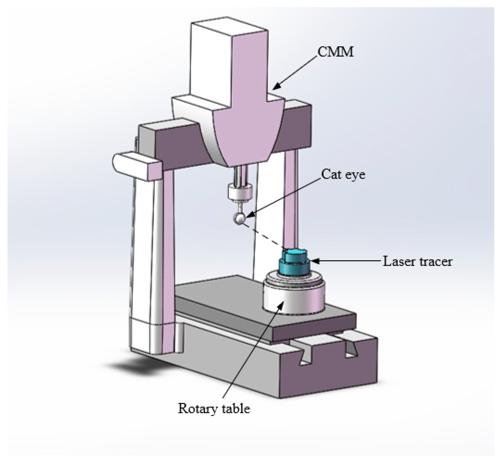
The laser tracer multi-station measurement model is shown in
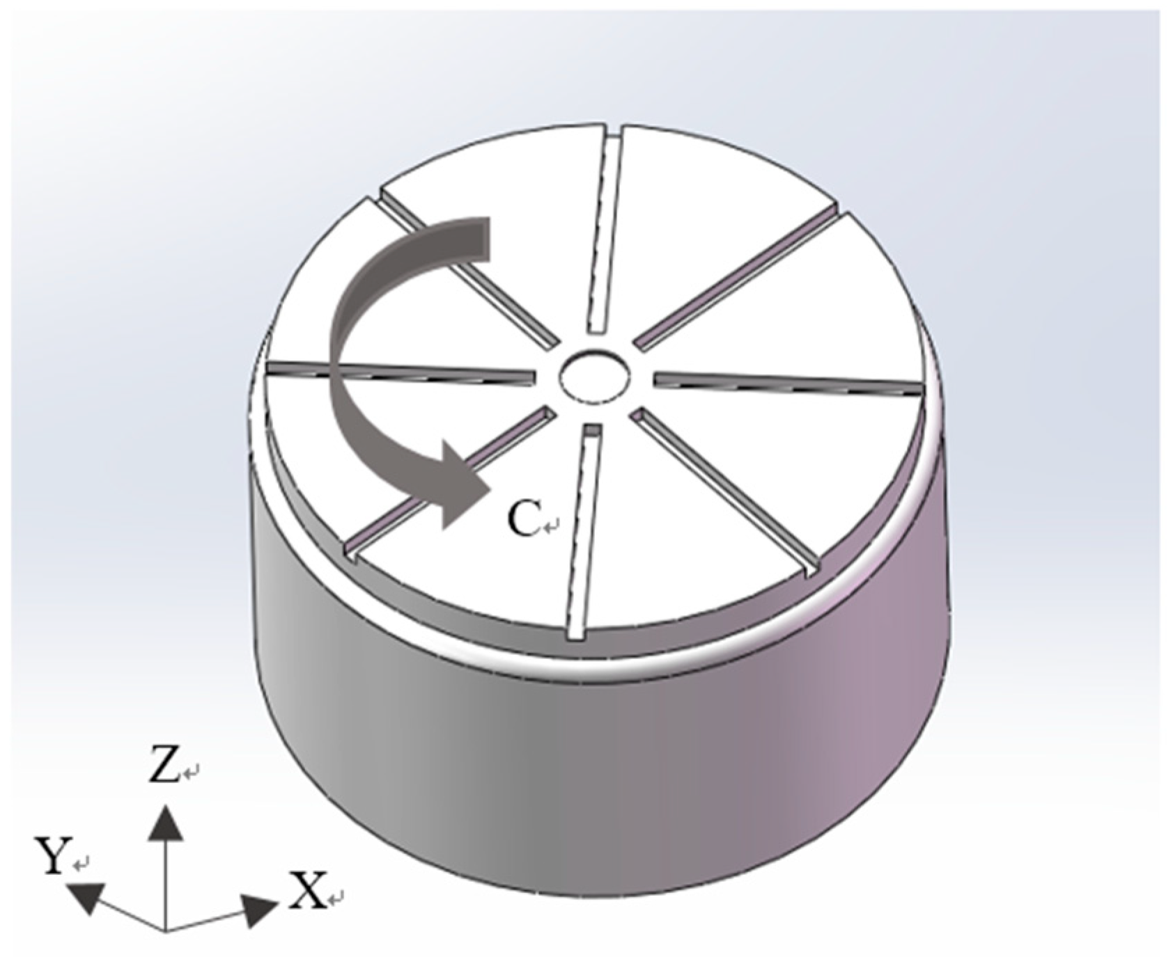
Figure 1. The rotary table is mounted on the working plane of the CMM (coordinate measurement machine), and the laser tracer is placed on the rotary table. The multi-station measuring system of the laser tracer consists of CMM, rotary table, and laser tracer. The coordinate system of the rotary table is the same as the coordinate system of the CMM, as shown in
Figure 2. The cat eye reflector of the laser tracer [
9,
10,
11] is fixed on the probe of the CMM as the measured point. The cat eye reflector has the same trajectory as the probe of the CMM. When the CMM controls the probe to move in the measurement space, the cat eye reflector also follows the probe of the CMM. The laser beam from the laser tracer is incident on the cat eye reflector and reflected back to the tracking head of the laser tracer. After receiving the reflected beam from the cat eye reflector, the laser tracer measures the relative displacement between the cat eye reflector (i.e., the measured point) and the laser tracer. The CMM provides the coordinates of measured points.
It is assumed that the laser tracer is used to measure
n measured points at
m stations. The coordinates of laser tracer stations are
Pj(
Xj,
Yj,
Zj); the coordinates of measured points are
Ai(
xi,
yi,
zi); the distance from the laser tracer at each station
Pj to the initial measured point
A1 is
dj; the high-precision interferometric length measured by the laser tracer is
lij. According to the distance formula of two points in three-dimensional (3D) space, the following relationship is established. The distance
dji of the laser tracer from each station to the measured point is obtained,
where
i = 1,2,3…
n,
j = 1,2,3,…
m.
Since
n measured points are measured at
m stations, according to Equation (1), the number of unknowns is 4
m + 3
n. In order to solve Equation (1), the following relationship should hold:
From Equation (2), we get m ≥ 4, n ≥ 16.
With the high-precision interferometric length measured by the laser tracer as the constraint condition, Equation (1) can be rewritten as the error equation,
Since Equation (3) is a nonlinear equation, it is difficult to directly solve it. According to a linearization method, the nonlinear function is converted into a linear function, which is then processed according to linear parameters. Let
be recorded as
Lij, and the first-order Taylor series expansion of Equation (3) is obtained as,
where
; the mark symbol
is the approximate of this value, and the approximate values
and
of the measured points in the actual calculation are replaced by the measured points in the coordinate system of CMM. Based on the singular value decomposition algorithm and the precision control threshold [
12], according to Equation (4), the correction values
of the measured points in CMM can be obtained.
3. Calibration Method for the Angular Positioning Deviation of the Rotary Table
3.1. Self-Calibration of Laser Tracer Station Based on Levenberg–Marquardt Algorithm
3.1.1. Self-Calibration Method
According to Equation (1), let
Record
, then
where
Rn is a set of
n-dimensional real numbers and
n is the number of measured points. The gradient of the objective function
F is denoted as
g(x), and we can obtain
where
.
In this paper, Levenberg–Marquardt algorithm (L-M) is used for iteration, and the coordinates of laser tracer stations and the distance from laser tracer stations to the initial measured point are obtained by iteration. The search direction of the iteration is set as
hi, then
where
μi > 0;
μi is the positive parameter introduced to adjust the search direction;
fi is the set of error equations;
Ji is the gradient matrix of error equations;
h is the set of search directions.
By optimality condition [
13,
14],
hi satisfies
where
I is
n × n identity matrix.
After solving Equation (9), we can get
where
Let
be the smallest non-negative integer satisfying Equations (11)–(14), then
where
and
.
In order to ensure that hi is the descending direction of fi(x) at xi, the initial value of μi is set at the beginning of iteration, and μi is adjusted continuously by calculating hi. According to the allowable error ε of the laser tracer multi-station measurement system, the coordinates Pj(Xj,Yj,Zj) of laser tracer stations and the distance dj from laser tracer stations to the initial measured point can be calibrated by iteration.
3.1.2. Selection of Parameter μi
The key of L-M algorithm is to select the parameter μ
i. According to the current iteration point, the quadratic function is assumed to be
where
Fi is the objective function.
The incremental ratio of objective function to quadratic function is expressed as
ri, then we can get
when
ri approaches 0 or 1, this parameter needs to be adjusted [
15]. Generally, the critical values of
ri are 0.25 and 0.75, so the selection rule of parameter
μi is obtained as
In the iteration process, the initial value of μi is given, and the value of each iteration step is taken as the initial value of the next iteration. According to the calculated hi and ri, the parameter μi is selected. Then, according to the selected parameter μi, hi is calculated, and the linear search is carried out to complete the iteration process.
3.2. Optimizing Coordinates of Laser Tracer Stations
In order to improve the accuracy of the coordinates of laser tracer stations obtained by the self-calibration algorithm, the Singular Value Decomposition (SVD) transformation [
16,
17] of the covariance matrix is used for plane fitting. The coordinates of
m laser tracer stations obtained by self-calibration algorithm are fitted into a plane. In the fitting plane, the distances from the coordinates of
m laser tracer stations to the fitting plane should have the minimum residuals. The optimized coordinates of laser tracer stations can be obtained by projecting
m coordinates of the laser tracer onto the fitting plane.
The principle of SVD of covariance matrix is provided as
where
U is the left singular orthogonal vector matrix; Σ is the diagonal singular value matrix;
V is the right singular orthogonal vector matrix.
The fitting plane is set as
The singular vector corresponding to the minimum singular value is the normal vector direction of the fitting plane equation.
By solving SVD, the fitting plane equation coefficients a, b, c, and e can be obtained, and then the fitting plane equation is obtained.
The optimized coordinates of laser tracer stations are set as . According to the parallelism between straight line and normal vector of the plane , the parametric equation of straight line is
After substituting into plane equation , we can get
After substituting λ into Equation (20), the optimized coordinates of laser tracer stations are obtained.
3.3. Calibration of The Angular Positioning Deviation of the Rotary Table
3.3.1. Solving the Center of the Circle of the Laser Tracer Station Coordinate Fitting Circle
Let the plane fitted by the
m station coordinates of the laser tracer obtained by the self-calibration algorithm be
γ. The center of the circle fitted by m station coordinates of laser tracer is
O(
xc,
yc,
zc). The projection equation of the plane formed by the plane γ at plane
z =
zc is set.
where
xc is the coordinate value of the center of the fitting circle in the X-axis direction;
yc is the coordinate value of the center of the fitting circle in the Y-axis direction, and
R is the radius of the fitting circle.
According to the principle of nonlinear least squares, the objective function can be defined as
Let
, then
In order to minimize the objective function
f, Equation (24) should satisfy the following conditions,
Let
,
,
and
, where
,
, then we can get
Based on Equation (26), we can get
According to Equation (27), we can get
According to Equation (19), we can get
In summary, the coordinates of the center of the circle fitted by the laser tracer O(xc,yc,zc) are obtained.
3.3.2. Calibration of the Angular Positioning Deviation of the Rotary Table
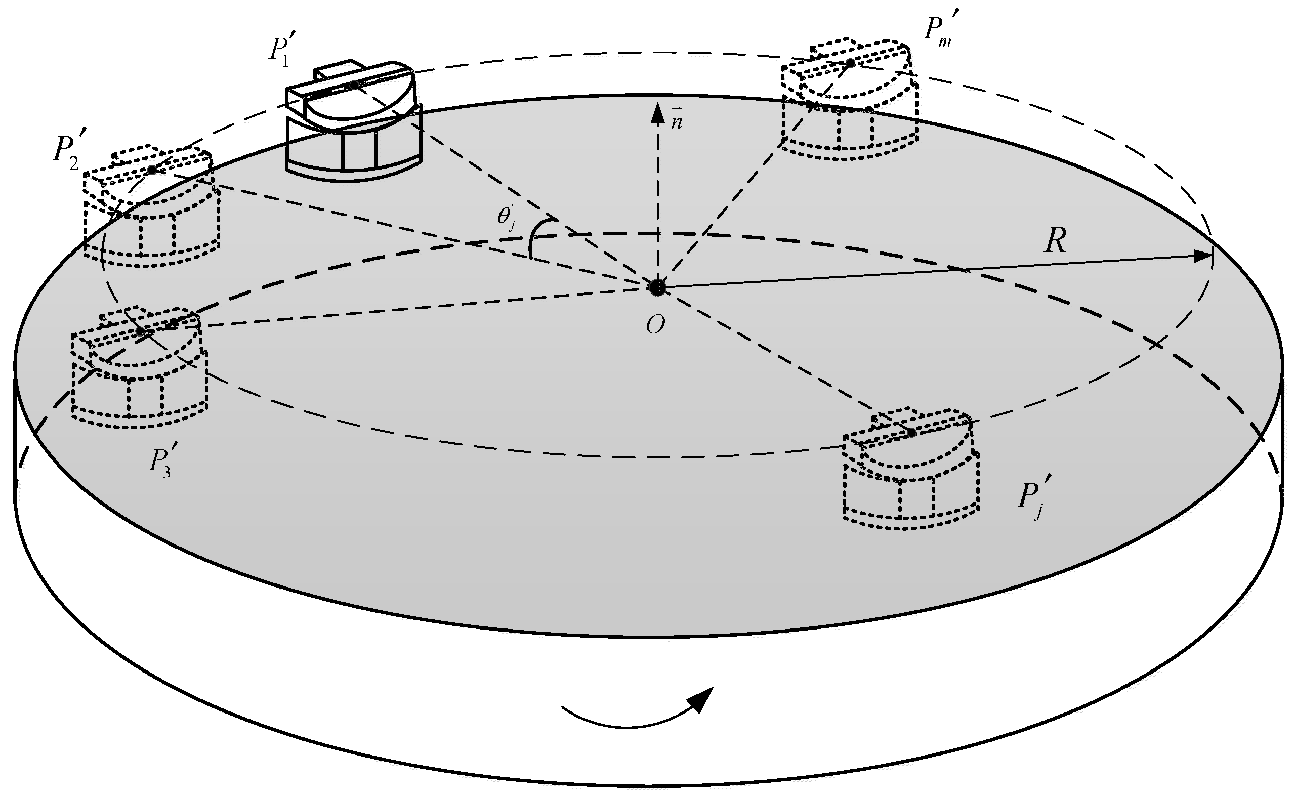
As shown in
Figure 3, the angle
between adjacent stations of the laser tracer is
where
is the coordinate of the j-th station optimized by the laser tracer;
is the coordinate of the j-th station optimized by the laser tracer, and
is the actual rotation angle of the rotary table.
Set the theoretical rotation angle of the rotary table as
θj. When the number of the coordinates of the laser tracer stations is
m, the rotary table rotates (
m − 1) times. According to Equation (32), the angular positioning deviation Δ
θj is obtained
where
θj. is the angle of theoretical rotation of the rotary table,
j = 1,2,3…
m − 1.
According to the multimeasurement averaging method, the angular positioning deviation of the rotary table based on the laser tracer multi-station measurement system is calibrated as
3.4. Algorithm Error of the Calibration Method of the Angular Positioning Deviation of the Rotary Table Based on the Laser Tracer Multi-Station Measurement System
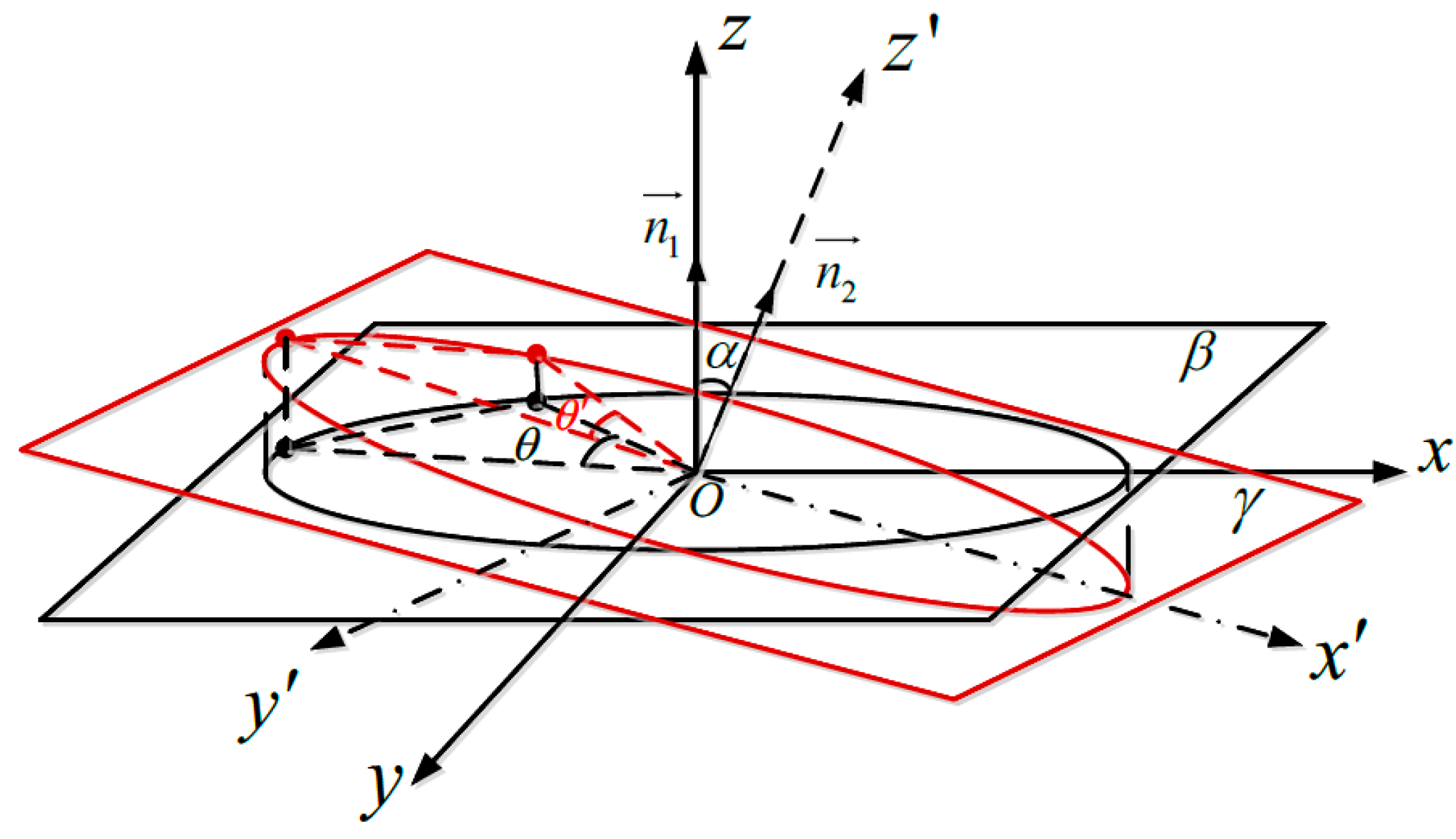
In the calibration process of the angular positioning deviation of the rotary table, it is assumed that the rotating axis of the rotary table is perpendicular to the plane of the table of the CMM. However, due to the squareness error of the X-axis or the Y-axis of the CMM, the rotating axis of the rotary table is not perpendicular to the plane of the CMM working plane. By comparing the working plane of the rotary table obtained by the coordinates fitting of the laser tracer multi-station with the CMM working plane, the algorithm error of the calibration method of the angular positioning deviation of the rotary table based on the laser tracer multi-station measuring system can be calculated.
The CMM working plane is
β, as shown in
Figure 4. The normal vector of the theoretical plane equation of the
β plane is
. The normal vector of the
γ plane is
. The angle between the
β plane and the
γ plane is
α, Then, we can get
where
a is the coefficient of the
X-axis direction of the fitting plane equation
γ;
b is the coefficient of the
Y-axis direction of the fitting plane equation
γ;
c is the coefficient of the
Z-axis direction of the fitting plane equation
γ.
According to the geometric relationship, the algorithm error Δ of the calibration method of the angular positioning deviation of the rotary table based on the laser tracer multi-station measurement system can be expressed as
4. Experimental Verification
4.1. Experimental System
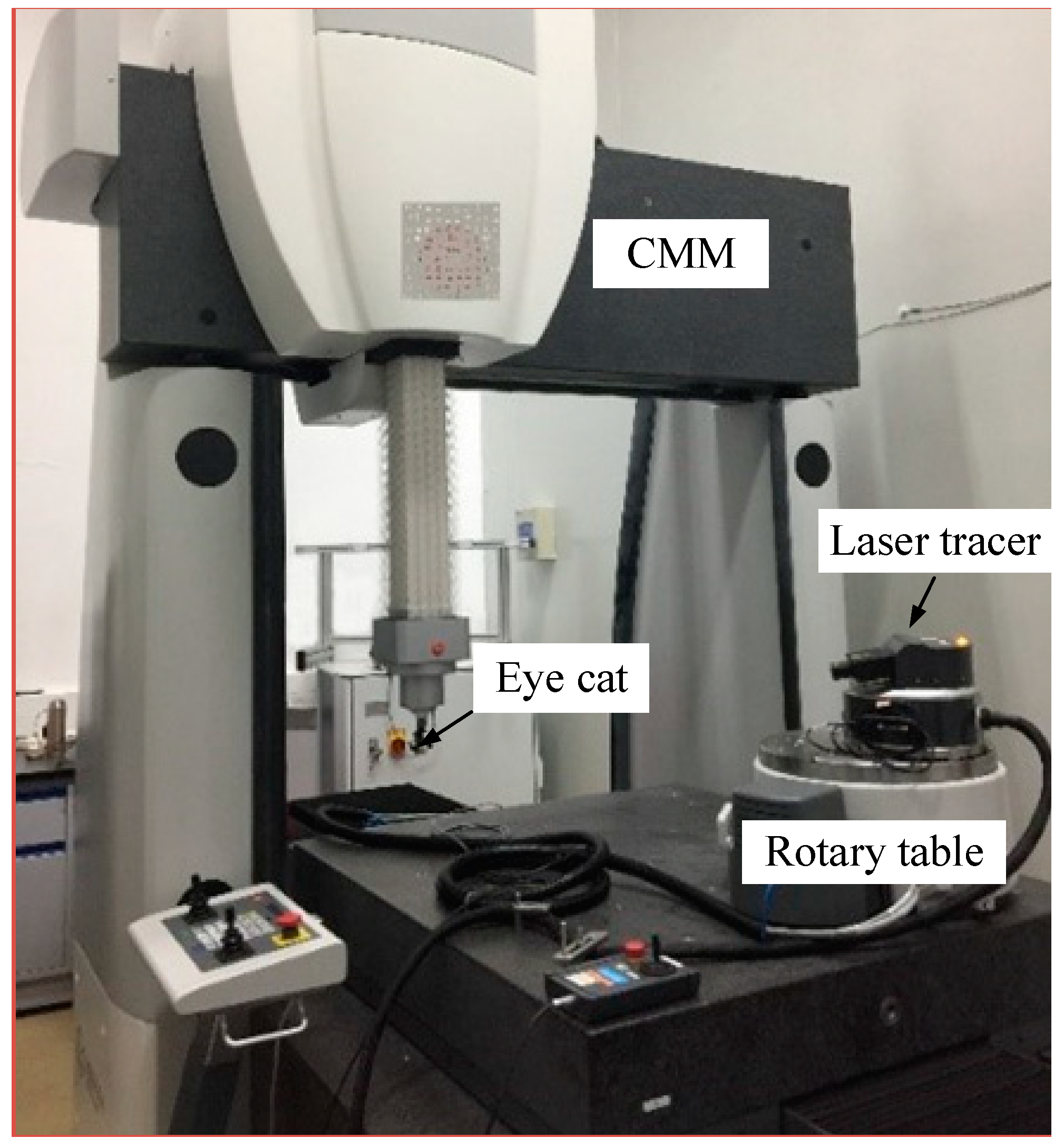
In order to verify the calibration method of the angular positioning deviation of the rotary table based on the laser tracer multi-station measurement system proposed in this paper, a multistation measurement system of laser tracer was built (
Figure 5). In the experiments, the measurement system was composed of the CMM (Leitz Infinity of Hexagon Company, Stockholm, Sweden), the high-precision rotary table (RT400, the angular positioning deviation = ±0.5″), and the laser tracer (Etalon Company, 07 2009 TR IF). The space range of the measured points in CMM was planned to be 450 × 600 × 450 mm
3. In this space range, the number of planned measured points was
n = 64, and the number of laser tracer stations was
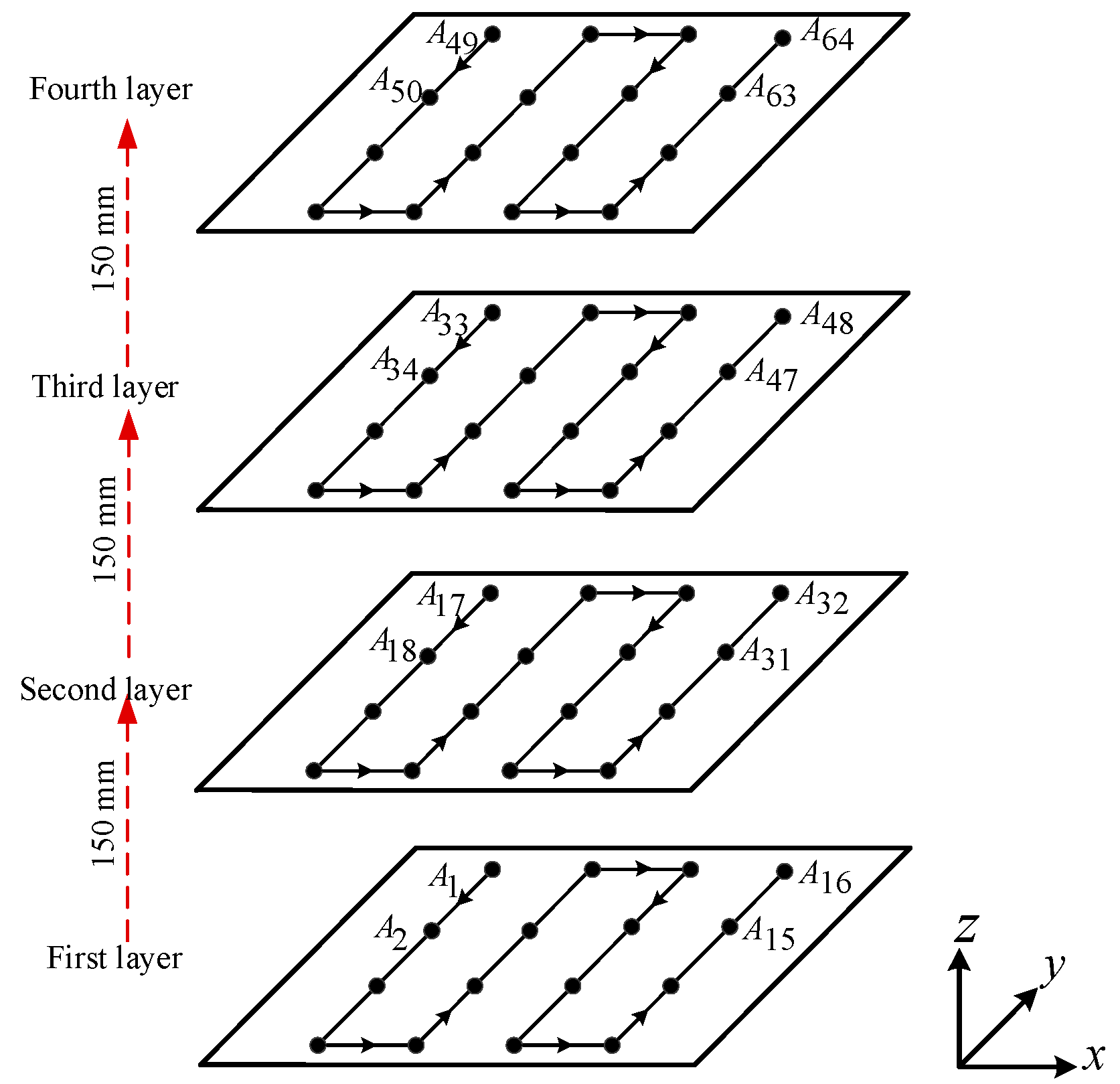
m = 11. The path planning of sampling points in the space range of the measured points is shown in
Figure 6. There were four layers of paths. The height of each layer varied by 150 mm with the same moving path.
In the calibration process of the angular positioning deviation of the rotary table, considering the light-tracing problem of the laser tracer at some positions, the laser tracer was fixed on the position of the rotary table of −145°. This position was recorded as the first position P1 of the laser tracer. The probe of CMM moved to A1. The rotary table rotated counterclockwise by 30°. The laser tracer rotated together with the rotary table. During the rotation process of the laser tracer from the first position P1 to the eleventh position P11, the interferometric length l1j of the laser tracer was respectively recorded. Then, the probe of CMM was controlled to move from A1 to A2 along the planned path in the measurement space. During the rotation process of the laser tracer from the first position P1 to the eleventh position P11, the interferometric length l2j of the laser tracer was respectively recorded. Then, the probe of CMM was controlled to move from point A1 to Ai along the planned path in the measurement space. During the rotation process of the laser tracer from the first position P1 to the eleventh position P11, the interferometric length lij was respectively recorded in turn. A total of 704 laser tracer interferometric lengths were recorded during the experiment.
4.2. Analysis of Experimental Results
4.2.1. Self-Calibration Coordinates of Laser Tracer Stations
The positioning precision of laser tracer is below 1 μm [
18]. The precision requirement of the laser tracer multi-station measurement system [
19] built in this paper was below 1 μm,
. Through a series of experiments for the parameters, the coordinates of calibrated laser tracer stations were observed, and the optimal setting of the parameters was obtained as:
β = 0.55 and
σ = 0.4. In the measurement system, the initial value
μi was set as
, where
,
,
, and
. Then
was calculated. According to Equation (17), these parameters follow the rules of
μi in L-M algorithm. According to the initial coordinate values
of the laser tracer, the initial distance
d0 from laser tracer to the initial measured point, and the selected parameters in L-M algorithm, the coordinates
of the laser tracer and the distance
from the laser tracer to the initial measured point were obtained by iteration (
Table 1).
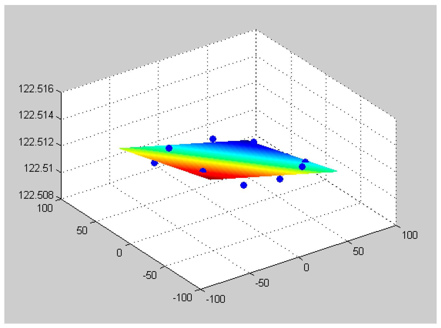
4.2.2. Fitting Plane of Station Coordinates and Coordinates of Optimized Stations
The plane vector corresponding to the minimum singular value in the SVD transform is the normal vector of the fitting plane equation. The coefficients of the plane equation (
) are
,
,
, and
, respectively. According to the results in
Section 3.2, the SVD transform of the covariance matrix was used for plane fitting, and the fitting plane was obtained (
Figure 7).
According to Equation (21) and the obtained values of the coefficients of the plane equation (
a,
b,
c,
e), λ = −0.0013 was calculated. The optimized coordinates of laser tracer stations are shown in
Table 2.
According to Equations (28)–(31), the coordinate of the center of the fitting circle (xc, yc, zc) is obtained as (−0.1434, −0.1396, 122.5119).
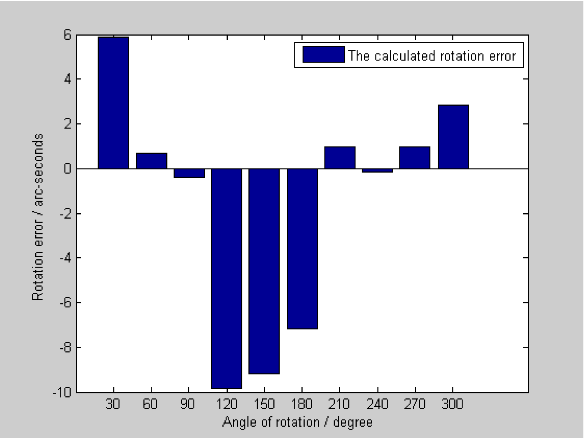
4.2.3. Angular Positioning Deviation of the Rotary Table
According to the calibration method of the angular positioning deviation of the rotary table based on the laser tracer multi-station measurement system proposed in this paper, the angular positioning deviations Δ
θj of the rotary table were obtained according to Equations (32) and (33) and provided in
Table 3. The angular positioning deviation of the rotary table at each indexing angle is shown in
Figure 8.
According to Equation (34), the angular positioning deviation of the rotary table based on laser tracer multi-station measurement is calibrated as
4.2.4. Algorithm Error of the Calibration Method of The Angular Positioning Deviation of the Rotary Table Based on the Laser Tracer Multi-Station Measurement System
According to Equation (36), with the above experimental data, the algorithm error of the laser tracer multi-station measurement system for calibrating the positioning accuracy of the rotary table was calculated as
5. Conclusions
In this study, the laser tracer multi-station measurement system was used to calibrate the angular positioning deviation of the rotary table. The algorithm error of the high-precision rotary table method based on the laser tracer multi-station measurement system was mainly analyzed. A laser tracer multi-station measurement system was built. The rotary table was mounted on the working plane of CMM, and the laser tracer was placed on the rotary table. The rotary table rotated with the same angle intervals. With the redundancy equation of the laser tracer multi-station measurement system, the nonlinear least squares method was used to self-calibrate the coordinates of laser tracer stations. The coordinates of laser tracer stations were iterated with the Levenberg−Marquardt algorithm. The singular value decomposition (Singular Value Decomposition) of the covariance matrix was used to fit the m coordinates of laser tracer stations obtained from the calibration algorithm to obtain a plane. Then m coordinates of laser tracer stations were projected onto the fitting plane to obtain the optimized coordinates of laser tracer stations. The circle was fitted with the coordinates of optimized laser tracer stations, and then the coordinates of the center of the fitting circle were solved. Then, the geometric relationship between the coordinates of optimized laser tracer stations and the center of the obtained fitting circle was established, and the actual rotation angle of the rotary table was obtained. In this way, the calibration of the angular positioning deviation of the rotary table was realized.
The experimental parameters were as follows. The spatial range of measured points given by CMM was 450 × 600 × 450 mm3; the number of measured points was 64; the number of laser tracer stations was 11; the angle range of rotary table was [−145°,155°]; the rotation angle interval of the rotary table was 30°. Under the above experimental conditions, the conclusions were drawn as follows: The angular positioning deviation of the rotary table was as low as compared with other work. Besides, the simple structure made it possible to meet the requirements of fast and efficient calibration. The algorithm error of the laser tracer multi-station measurement system for calibrating angular positioning deviation of the rotary table was . The experiment proved the feasibility of the proposed calibration method. In actual industrial measurement, the angular positioning deviation demand of high-precision rotary tables is low.
Although there is a limitation for this case that the rotary table should not be linked with the CMM, it is especially suitable for calibration of angular positioning deviation of large high-precision rotary tables. It also makes a theoretical preparation for the calibration of four-axis machine tools.
Author Contributions
Data curation, H.C. and B.J.; Investigation, H.C.; B.J. and H.L.; Methodology, H.C. and B.J.; Resources, Z.S.; Writing—original draft, S.Z., H.S. and Y.S.; Writing—review & editing, S.Z., H.S. and Y.S.
Funding
The research was funded by National Key Research and Development Program “Making basic technology and key components” special project under Grant No. 2018YFB2001402, Natural Science Foundation of Beijing, China under Grant No.3182005, National Natural Science Foundation of China under Grant No. 51635001.
Conflicts of Interest
The authors declare no conflict of interest.
References
- Ji, H.J.; Gyungho, K.; Jeong, S.O.; Sung, C.C. Method for measuring location errors using a touch trigger probe on four-axis machine tools. Int. J. Adv. Manuf. Technol. 2018, 99, 1003–1012. [Google Scholar]
- Chen, Y.T.; More, P.; Liu, C.S. Identification and verification of location errors of rotary axes on five-axis machine tools by using a touch-trigger probe and a sphere. Int. J. Adv. Manuf. Technol. 2019, 100, 2653–2667. [Google Scholar] [CrossRef]
- Zeng, M.; Wang, J.H.; Zhang, J.; Su, B.K. Study on the gauging method in the angler measuring system of turntable. J. Chin. Inert. Technol. 1998, 6, 84–88. [Google Scholar]
- Xu, T.; Li, B.; Liu, T.X.; Xue, L.T.; Chen, T. Initial calibration of tracking turntable for vehicle-borne opto-electronic tracking system. Opt. Precis. Eng. 2013, 21, 782–789. [Google Scholar]
- Wang, M.; Bao, J.P. Research and implementation of accuracy calibration method for large turntable. Ind. Meas. 2014, 24, 31–32, 35. [Google Scholar]
- Bai, P.J.; Xue, N.; Liu, S.T.; Song, T.; Li, J.H. Angular calibration method of precision rotating platform based on laser tracker. J. South China Univ. Technol. (Nat. Sci. Ed.) 2016, 44, 100–107. [Google Scholar]
- Pi, S.W.; Liu, Q.; Sun, P.P. Geometric error detection for rotary feed drive based on laser interferometer. Chin. J. Sci. Instrum. 2017, 38, 2484–2491. [Google Scholar]
- Yan, Y.Y.; Liu, W.; Fu, J.J. Compensation for adjustment error in high positioning accuracy angular positioning deviation turntable measuring system. J. Jilin Univ. (Eng. Technol. Ed.) 2017, 47, 855–860. [Google Scholar]
- Ostrowska, K.; Gaska, A.; Kupiec, R.; Sladek, J.; Gromczak, K. Verification of Articulated Arm Coordinate Measuring Machines Accuracy Using LaserTracer System as Standard of Length. MAPAN J. Metrol. Soc. India 2016, 31, 241–256. [Google Scholar] [CrossRef]
- Schwenke, H.; Schmitt, R.; Jatzkowski, P.; Warmann, C. On-the-fly calibration of linear and rotary axes of machine tools and CMMs using a tracking interferometer. CIRP Ann. Manuf. Technol. 2009, 58, 477–480. [Google Scholar] [CrossRef]
- Schwenke, H.; Franke, M.; Hannaford, J.; Kunzmann, H. Error mapping of CMMs and machine tools by a single tracking interferometer. CIRP Ann. Manuf. Technol. 2005, 54, 475–478. [Google Scholar] [CrossRef]
- Timonthy, S. Numerical Analysis, 2nd ed.; China Machine Press Xicheng District: Beijing, China, 2017. [Google Scholar]
- Yuan, Y.X.; Sun, W.Y. Optimization Theory and Methods; Science Press Dongcheng District: Beijing, China, 2016. [Google Scholar]
- Yuan, Y.X. Nonlinear Optimization Calculation Method; Science Press Dongcheng District: Beijing, China, 2017. [Google Scholar]
- Ma, C.F.; Ke, Y.F.; Xie, Y.J. Optimization Calculation Method and Matlab Program Implementation; National Defense Industry Press Haidian District: Beijing, China, 2017. [Google Scholar]
- Qiao, Z.J.; Pan, Z.J. SVD principle analysis and fault diagnosis for bearings based on the correlation coefficient. Meas. Sci. Technol. 2015, 26, 085014. [Google Scholar] [CrossRef]
- Sun, H.C.; Fang, L.; Guo, J.Z. A fault feature extraction method for rotating shaft with multiple weak faults based on underdetermined blind source signal. Meas. Sci. Technol. 2018, 29, 125901. [Google Scholar] [CrossRef] [Green Version]
- Fan, B.J.; Li, G.Y.; Yi, W.G.; Yang, Z. The Measurement Principle and Application of Laser Tracker Surveying and Mapping; Press Xicheng District: Beijing, China, 2017. [Google Scholar]
- Chen, H.F.; Jiang, B.; Shi, Z.Y.; Sun, Y.Q.; Song, H.X.; Tang, L. Uncertainty modeling of the spatial coordinate error correction system of the CMM based on laser tracer multi-station measurement. Meas. Sci. Technol. 2019, 30, 025007. [Google Scholar]
© 2019 by the authors. Licensee MDPI, Basel, Switzerland. This article is an open access article distributed under the terms and conditions of the Creative Commons Attribution (CC BY) license (http://creativecommons.org/licenses/by/4.0/).


