Article

Minimum Frequency and Voltage Stability Constrained Unit Commitment for AC/DC Transmission Systems

State Grid Jiangsu Electric Power CO., LTD. Research Institute, Nanjing 211103, China
*
Author to whom correspondence should be addressed.
Appl. Sci. 2019, 9(16), 3412; https://doi.org/10.3390/app9163412
Submission received: 11 July 2019 / Revised: 15 August 2019 / Accepted: 15 August 2019 / Published: 19 August 2019
(This article belongs to the Special Issue Control and Operation of AC and DC Systems)

Abstract

:
An increased use of the high-voltage direct current (HVDC) technologies can have important effects on frequency performance and voltage stability of the receiving-end grid during normal operation as well as during blocking failure. The main reasons are the inherent characteristics of the HVDC such as its much larger capacity than thermal plants and lack of voltage supporting ability to the alternating current (AC) grid. These has led to new challenges for AC/direct current (DC) power grid operators in terms of ensuring power system security. To address these challenges, a unit commitment (UC) of the receiving-end in the AC/DC hybrid grid is presented in this paper. In the proposed model, primary frequency modulation constraints are added to provide sufficient capacity for HVDC blocking. Besides, grid security constraint after secondary frequency regulation is also considered because HVDC blocking failure would cause large range power transfer and transmission lines overload. Meanwhile, voltage stability constraints are employed to guarantee enough voltage supporting capacity from thermal plants at the HVDC feed-in area. Based on the characteristics of the model, Benders decomposition and mixed integer programming algorithm are used to get the optimal transmission power of the HVDC and schedule of thermal units. The study is done by considering the IEEE-39 and Jiangsu power grid in eastern China, containing two HVDC transmission projections respectively. The results are also validated by simulation of different HVDC blocking failure scenarios.

1. Introduction

The high-voltage direct current (HVDC) system can not only transmit high-capacity power in long-distance, but also regulate power flexibly based on multiple control modes [1,2]. At the present time, the line-commutated converter (LCC) and voltage source converter (VSC) [3] are two main technologies for HVDC transmission. However, in China, LCC-HVDC has dominated the scene of high-capacity power transportation and plays an important role in transmitting renewable power from the power supply region to heavy load centers. As more LCC-HVDC projects were put into operation, how to operate them to guarantee stability and improve economy of the power grid became a problem which need to be solved urgently.
In recent years, some effort has been spent by power engineers and researchers to investigate the optimum operation scheme of the alternating current /direct current (AC/DC) hybrid power system, such as researching the transmission power limits with temperature [4,5,6]. The simplest approach is to treat HVDC transmissions as constant power injections or withdrawals. Then the existing mature models and algorithms of unit commitment (UC), economic dispatch (ED), and optimal power flow (OPF) can still be suitable for the AC/DC hybrid grid. However, such simplified technology ignores HVDC’s operational characteristic and the interaction between the AC and DC system. Another method is establishing the detail model of the HVDC during operation optimization. For example, authors in [7] introduced comprehensive representation of HVDC transmission in operation optimization of the AC/DC hybrid system while increasing the complexity of the model. To solve such problem efficiently, linear power flow equations were used to model the AC and DC transmission grids so as to decrease the complexity of the whole model in [8]. Another method is utilizing Benders decomposition (BD) algorithm to decompose the large scale model into a master problem and several sub-problems. Then the economic dispatch problem can be solved by efficient iterative algorithms [9]. Similarly, authors in [10,11,12] obtained a solution for the security-constrained unit commitment (SCUC) problem more effectively with BD. In addition, the annealing algorithm, which is used as the solver of the planning model containing bundled wind-thermal generation and the HVDC, belongs to the field of artificial intelligence optimization algorithms [13].
Despite the hybrid AC/DC power system, operation could be improved partly by the above achievement, it is worth pointing out that there are still some significant challenges in the receiving-end of hybrid grids to overwhelm:
(i)
Low frequency risk. HVDC blocked accident is one of the most serious faults in the operation. It can always be triggered by continuous commutation failures or DC lines failures. With such wind power as random source penetrating into the power grid, the HVDC blocked risk will increase [14]. After HVDC transmissions are fed into the power grid, the system operator should prepare much more spinning reserve for dealing with its blocked fault because of HVDC’s larger capacity than thermal plants. Meanwhile, renewable power transferred by the HVDC is preferred to traditional fossil fuel, resulting in less online thermal plants, which are currently the main reserve power providers. On account of increasing reserve demand and decreasing reserve suppliers, low frequency fault might happen after the HVDC is blocked. For example, Jinsu’s HVDC bipolar block on 19 September 2015 lead to grid frequency in eastern China, reducing to 49.557 Hz, violating the minimum frequency requirement.
(ii)
Voltage stability problem [15]. For the purpose of consuming power easier in the receiving-end grid, HVDC systems are always fed into the metropolitan area with heavy load and fewer power plants. Such feature lead to lower voltage and weak voltage support ability. In addition, based on switching the devices’ characteristic, LCC-HVDC need lots of reactive power while transmitting active power massively. Although AC filters are usually configured in converter stations, a great quantity reactive power is absorbed by LCC-HVDC during commutation failure fault. These further deteriorate voltage stability of the AC grid.
To overcome the above challenges, this paper presents a UC model for the receiving-end in the AC/DC hybrid grid. The proposed model contains minimum frequency constraints for ensuring sufficient capacity on primary frequency regulation after the HVDC blocked. Moreover, transmission line power limits after completing secondary frequency regulation are also included because of large power translation caused by the same fault. Besides that, voltage stability constraints are added to guarantee the voltage supporting ability in the grid near the HVDC. It is worth mentioning that HVDC power is variable, participating in optimal dispatching of the power grid. Based on characteristics of the model, Benders decomposition and the mixed integer programming algorithm are used to get the optimal transmission power of the HVDC and planning of thermal generators.
The rest of the paper is structured as follows. Section 2 and Section 3 model the SCUC formulation with AC/DC transmission constraints and Benders decomposition-based solution presented in Section 4. The proposed algorithm is tested with the IEEE 39-bus and Jiangsu power grid in eastern China in Section 5. We summarize the conclusion in Section 6.

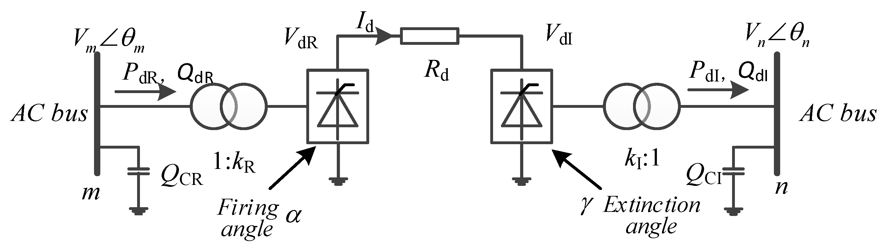
2. HVDC Transmission System Model

HVDC transmission systems consist of at least two converters (i.e., rectifiers and inverters) and overhead lines that link converters. For the sake of diminishing harmonics generated by AC/DC hybrid systems, AC filters are installed on the AC side of DC terminals. In this section, we review DC transmission systems and corresponding DC power flow equations for our UC formulation.

2.1. LCC-HVDC Model

Figure 1 presents a typical LCC-HVDC system which is connected to AC bus m and n through coupling transformers. In order to model the HVDC which is linked to the AC system, seven converter variables, i.e., VdR, VdI, Id, kR, KI, α, and γ are considered in Figure 1. These variables determine the HVDC operating state.
The whole HVDC is modeled by Equations (1)–(7). The converter Equations (1) and (2) express VdR (VdI) in terms of Vm (Vn), kR (kI), α (γ), and other converter variables while the coupling transformers are assumed to be lossless. Equation (3) represents the DC voltage-current relationship which depends on the DC transmission system configuration (i.e., VdR, VdI, and Id). After getting the active power of both rectifier and inverter by Equations (4) and (5), the exchange reactive power between AC and DC system could be calculated through Equations (6) and (7) by considering reactive compensation capacity QCI and QCR.
V d R = 3 2 π n R k R V m cos α 3 π n R X c , R I d
V d I = 3 2 π n I k I V n cos γ 3 π n I X c , I I d
V d R = V d I + R d I d
P d R = V d R I d
P d I = V d I I d
Q d R = Q C R ( V d R + 3 π n R X c R I d ) 2 I d 2 cos 2 α P d R 2
Q d I = Q C I ( V d I + 3 π n I X c I I d ) 2 I d 2 cos 2 γ P d I 2
Each LCC-HVDC (rectifier or inverter) is regulated by two out of five control modes. The modes are as follows.
(1)
Constant current (CC).
Id = const
(2)
Constant voltage (CV).
VdI = const
(3)
Constant power (CP).
PdR = VdRId = const
(4)
Constant firing angle (CFA).
α = const
(5)
Constant extinction angle (CEA).
γ = const
Usually, two control modes are selected to maximize the economic benefits of HVDC transmission systems while keeping all variables within their limits. In this paper, CP is used in rectifier, meanwhile CV is preferred to the inverter.
At the situation of the per-unit system, nodal power balance equations at the AC bus m that is linked to converter l are showed as Equations (8) and (9). The sign of Ptd,l depends on rectifier or inverter. Ptd,l is decided by the state of converter and reactive power compensation.
0 = P L , m t ± l m P d , l t + V m t n m V n t ( G m n cos θ m n t + B m n sin θ m n t )
0 = Q L , m t + l m Q d , l t + V m t n m V n t ( G m n sin θ m n t B m n cos θ m n t )
m N B , t T

2.2. Minimum Frequency Limit Constraints

1. Primary frequency regulation capacity for HVDC N-1 fault
As we all know, HVDC’s rated capacity is much larger than thermal generators. It means that if any HVDC blocked, larger power deficiency and low frequency would emerge in the power system. Therefore, enough primary frequency regulation capacity for HVDC’s N-1 fault is critical to keep frequency within limit. Constraints (10) and (11) describe that when the largest capacity HVDC blocked, the power grid’s frequency would drop less than Δfmax, meeting the operation requirement.
( i N G K G , i × u i t + K L ) × Δ f max P ¯ d t ,    i T
P ¯ d t = max { P d , 1 t , P d , 2 , t P d , N L t }
2. Security constraint after secondary frequency regulation
When HVDC blocking fault happens, secondary frequency regulation would dispatch generators to re-achieve power balance at each bus, as shown in constraints (12) and (13). Meanwhile, the power’s wide transfer would occur and result in transmission lines’ power exceeding limits. To avoid the above situation, we introduce constraint (14) in the UC model.
i N m ( P G , i t + Δ P G , i , s t ) × u i t = P L , m t + V m , s t n m V n , s t ( G m n cos θ m n , s t + B m n sin θ m n , s t )
i N m ( Q G , i t + Δ Q G , i , s t ) × u i t = Q L , m t + V m , s t n m V n , s t ( G m n sin θ m n , s t B m n cos θ m n , s t )
P L m n , min P L m n , s t P L m n , max ,     m n N B , t T

2.3. Voltage Stability Constraints

Constraints (15) and (16) are added in the proposed model to ensure the static voltage stability margin of load center is greater than η min . The reason is that the load center of the power grid always has weaker voltage supporting ability. Besides that, HVDC also needs enough voltage support capacity to operate steadily. Therefore, enough generators close to inverter substation could start up by the voltage stability constraints and provide necessary reactive power by following constraints.
η V S M > η min
η V S M = ( P l * P l 0 ) / P l 0

3. SCUC with HVDC Constraints

3.1. Objective Function

The objective function aims to minimize the system operation cost. It comprises two terms: The sum of the total generation costs, and start-up cost of each generator, as follows:
min C s u m = t T i N G [ C i ( P G , i t ) × u i t + S T i t × u i t ( 1 u i t 1 ) ]

3.2. UC Constraints

3.2.1. Generating Unit Constraints

1. Generating unit capacity
Constraints (18)–(21) ensure that generators operate between their minimum and maximum allowed outputs, while the overall output is dependent on both rated minimum power output and ramp-down limit of generating unit.
P _ i , min P G , i t + r i t P ¯ i , max
P _ i , min = max ( P _ G , i , min , P G , i t 1 60 × D R i )
P ¯ i , max = min ( P ¯ G , i , max , P G , i t 1 + 60 × U R i )
Q _ G , i , min Q G , i t Q ¯ G , i , max
2. Minimum ON/OFF status constraints
The next constraints are minimum up and down time constraints of generators, which use different start-up states, depending on the time a generator had been ON or OFF before being started.
{ u i t = 1 ,      i f      T i , o n t 1 < T i , u p u i t = 0 ,      i f      T i , o f f t 1 < T i , d o w n u i t = 0 or 1      o t h e r s
3. Generator start-up cost function
The start cost is modeled by the following constraint (23). It is divided into hot-start and cold-start, depending on OFF time and minimum OFF time of the generator.
{ S T i t = H S T i , i f T i , d o w n T i , o f f t T i , c o l d + T i , d o w n S T i t = C S T i , i f T i , o f f t T i , c o l d + T i , d o w n
i N G , t T

3.2.2. Security Constraints of AC Power System

1. Power balance of buses
Constraints (24) and (25) are the power balance at each bus m and at each time period t. It balances the power generated by generators, power inflows with the demand and power outflows.
i N m P G , i t × u i t = P L , m t + V m t n m V n t ( G m n cos θ m n t + B m n sin θ m n t )
i N m Q G , i t × u i t = Q L , m t + V m t n m V n t ( G m n sin θ m n t B m n cos θ m n t )
m n N B , t T
2. Transmission power constraints
Equation (26) computes power flows through lines between bus m and n, while constraint (27) limit theses power flows.
P L m n t = V m t V n t sin θ m n t / X m n
P L m n , min P L m n t P L m n , max , m n N B , t T
3. Bus voltage constraints
Constraint (28) denotes that voltage of bus m would fluctuate between their allowed ranges.
V m , min V m t V m , max , m N B , t T
In conclusion, Formulas (1–28) constitute the whole SCUC model for the AC/DC hybrid system. Compared with the existing UC models, Formulas (10–14) not only keep minimum frequency higher than minimum frequency requirement when HVDC blocking happens, but also avoid transmission lines’ power due to the power’s wide transfer after secondary frequency regulation; meanwhile the constraints shown in Formulas (15) and (16) ensure voltage stability in the power grid near HVDC. As a result, the optimal scheduling of the introduced UC model could improve the reliability and economic efficiency of the AC/DC hybrid power grid.

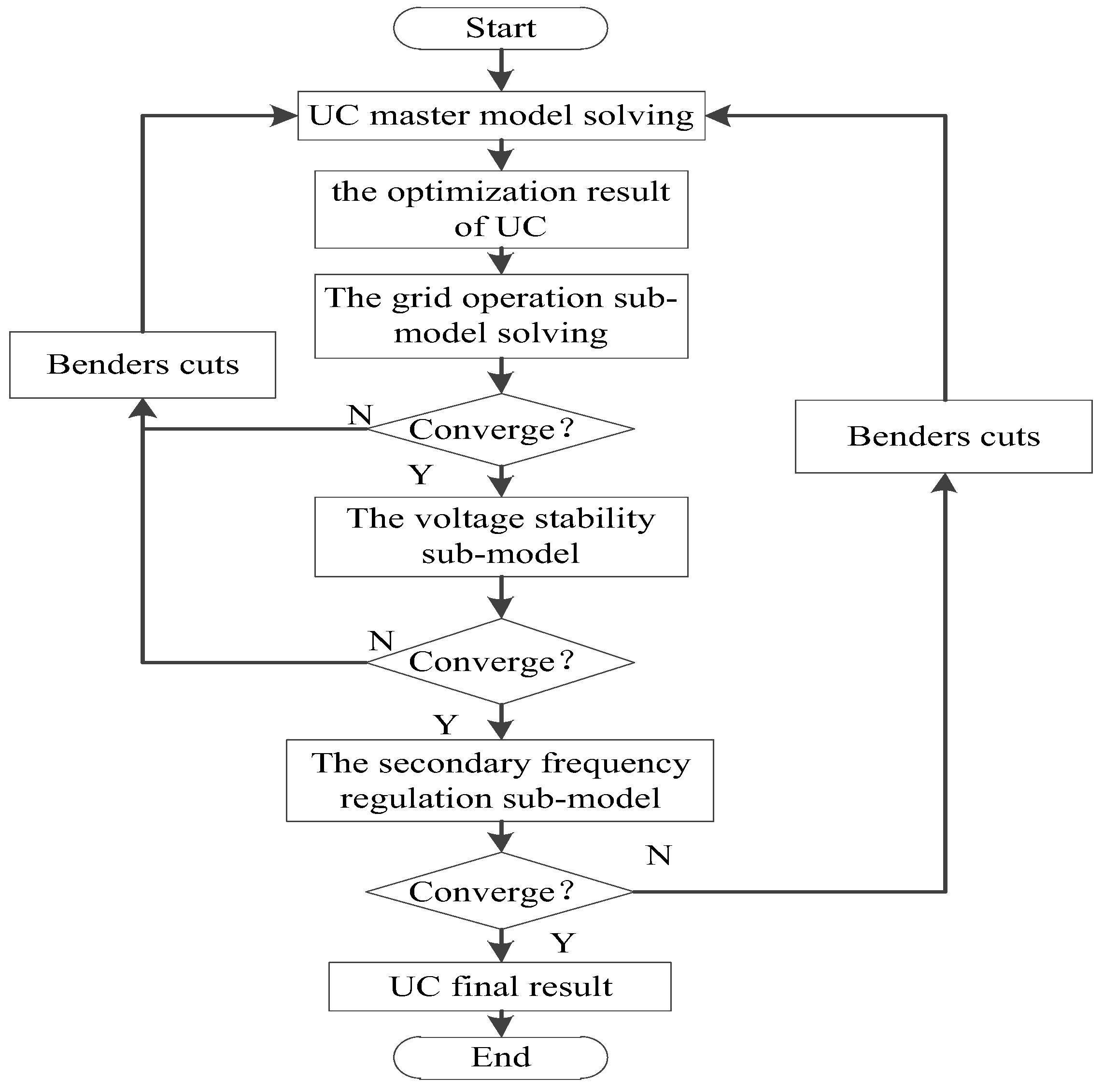
4. Model Decomposition and Solution

The proposed AC/DC hybrid SCUC model is composed of generating unit constraints, security constraints of the AC power system, minimum frequency limit constraints for HVDC’s N-1 fault, and the constraints of static voltage stability margin for the heavy load center. Obviously, it is a typical NP-hard problem and difficult to directly solve. In this section, we decompose the whole model into the UC master model, SC sub-model, and voltage stability constraint sub-model. Then, based on the linearization algorithm of UC introduced in literature [16], the master model and all sub-models are linearized respectively. The coordination mechanism is established between the master model and all sub-models by the Benders decomposition theory. When the generators schedule of the master model simultaneously satisfy the verification calculation of three sub-models, the global optimum solution is obtained.

4.1. UC Master Model

The master model is the traditional UC model with HVDC transmissions, which is composed of objection Function (17), minimum frequency limit Constraints (10) and (11), generating units’ Constraints (18)–(23) and Benders cut constraints generated from all three sub-models. Besides, Constraint (29) is taken into account to realize power balance.
i N G P G , i t × u i t P L , s u m t + P l o s s t
After linearizing the objective function and constraints in the master model, the mixed integer programming method is employed to solve the problem. The master model aims to get optimization of the generators’ ON/OFF and power output variables, HVDC transmission power, which would be used as constant in the sub-models. The specific calculation process can be seen in literature [16].

4.2. Security Constraints Sub-Model

This sub-model is used to validate whether the optimization result of the UC master model satisfies the operating constraints in the hybrid AC/DC power system. In essence, the process is equal to the calculation of the power flow with HVDC operational constraints, generator reactive power constraint, bus voltage, and transmission power limits. This paper solves such problem by the traditional Newton–Raphson method which is transformed into successive linear programming. The advantage is that the Benders cut could be formed conveniently, as shown in Formulas (30)–(39). Among these variables, MP1 (MP2), MQ1 (MQ2), MPL1 (MPL2), and MPD1 (MPD2) are non-negatively and used to relax equations of the AC/DC hybrid power flow calculation.
Among formulas, Formula (31) is the linear equation of buses active and reactive power; Formula (32) is the linear equation of the active and reactive power of the HVDC transmission system; Formula (33) is the linear equation of line active power; Formulas (34)–(37) are the upper and lower limits of generator active and reactive power, transmission power and buses voltage; Formulas (38) and (39) are the upper and lower limits of the relevant AC/DC variables in the HVDC transmission system. We use H, N, J, L, O, D, E, F, Z, S as the first derivative coefficient matrix of the corresponding equation to independent variables. In addition to the equilibrium node, the active increment of other nodes should meet Formula (34). Λ, ψ _ and ψ ¯ are the corresponding simplex multiplier of the constraints.
M i n    w t = ( M P 1 + M P 2 ) + ( M Q 1 + M Q 2 ) + ( M P L 1 + M P L 2 ) + ( M P D 1 + M P D 2 )
[ Δ P G Δ Q G ] + [ H N J L ] [ Δ θ Δ V ] + [ Δ P d c Δ Q d c ] + [ M P 1 M Q 1 ] [ M P 2 M Q 2 ] = [ d P d Q ]
[ Δ P d c Δ Q d c ] + [ O D E F ] [ Δ X a c Δ X d c ] + [ M P 1 D M Q D 1 ] [ M P D 2 M Q D 2 ] = [ d P d c d Q d c ]
Δ P L + [ Z S ] [ Δ θ Δ V ] + M P L 1 M P L 2 = d P L
Δ P G = 0         λ
Δ Q min Δ Q Δ Q max         ψ _ , ψ ¯  
Δ P L min Δ P L Δ P L max
Δ V min Δ V Δ V max
Δ X a c , min Δ X a c Δ X a c , max
Δ X d c , min Δ X d c Δ X d c , max
The process of solving the sub-model is as follows [17]:
Step1:
Set up the maximum permissible error ε and the maximum iteration number ITmax. Set iter = 1, then, initialize bus real and reactive power injection and buses voltage;
Step2:
Calculate coefficient matrix and right-end unbalance value in Formulas (31)–(33) and the upper and lower limits of the variables in Formulas (34)–(39);
Step3:
Solve the above models with the linear programming method and obtain ΔP, ΔQ, Δθ, ΔV, ΔPdc, ΔQdc, ΔXac, ΔXdc, and all relaxation variables;
Step4:
Update all variables; if min (ΔP, ΔQ, Δθ, ΔV, ΔPdc, ΔQdc) ≤ε or iterITmax, the calculation is over; or iter = iter + 1, return to step 2.
After several calculations of the linear programming problem, if the objective function wt = 0 at the time interval t, the generator ON/OFF and real power output could satisfy operating constraints; otherwise Benders cut constraints, as shown in constraint (40), would be formed and supplied to the master model for recalculation.
w t + i N G λ i × ( P G , i t ( P G , i t ) * ) + i N G ψ ¯ × Q G , i , m a x × ( u i t ( u i t ) * ) + i N G ψ _ × Q G , i , m i n × ( u i t ( u i t ) * ) 0
Because of Benders cuts, new solution of generators’ ON/OFF and real power output would be forced to eliminate w t as much as possible. By repeating this process in such way, the optimal generators’ ON/OFF and active power are finally obtained.

4.3. The Voltage Stability Sub-Model

This sub-model is established to deal with voltage stability constraints for heavy load center. To improve solving efficiency, this paper adopts the following method: Firstly, according to ηmin in Formula (15), we get ultimate load Pl* by Equation (41); then real load of buses in heavy load center and all generators’ power output except heavy load center could be increased separately; finally, power flow calculating is processed to verify whether it is convergent. If convergent, it means the UC optimization result satisfies the voltage stability constraint; if not, the new Benders cut should be generated and added to the UC master model, which would be re-solved.
P l * = ( 1 + η min ) × P l 0
M i n w t = ( M P 1 + M P 2 )
[ Δ P G Δ Q G ] + [ H N J L ] [ Δ θ Δ V ] + [ Δ P d c Δ Q d c ] + [ M P 1 M Q 1 ] [ M P 2 M Q 2 ] = [ d P d Q ]
[ Δ P d c Δ Q d c ] + [ O D E F ] [ Δ X a c Δ X d c ] + [ M P 1 D M Q D 1 ] [ M P D 2 M Q D 2 ] = [ d P d c d Q d c ]
Δ P G = 0         λ
Δ Q min Δ Q Δ Q max         ψ _ , ψ ¯  
Δ X a c , min Δ X a c Δ X a c , max
Δ X d c , min Δ X d c Δ X d c , max
Benders cut constraints will be generated as shown in Formula (37) when wt is not equal to zero after several calculations.

4.4. The Secondary Frequency Regulation Sub-Model

After HVDC blocking happens, the secondary frequency regulation would adjust real power output of thermal generators to re-establish power balance in a short time. The constraints in Formulas (12)–(14) are added in order to ensure transmission active power within limits. To get augmentation Δ P G , i t and Δ Q G , i t of the real and reactive power of the thermal generators, the linear model of the secondary frequency regulation sub-model is established, which is displayed in Appendix A in detail.
The method to solve the linearization of the secondary frequency regulation sub-model is same as the algorithm described in the last section. When w t = 0 , power grids meets power flow calculation convergence, and transmission power limits requirement at the same time after secondary frequency regulation; when w t > 0 , it means that transmission power are out of limit and Benders cut constraints should be formed, then return to the master model for recalculation.
The calculation process of the UC master model and three sub-models is shown in Figure 2.

5. Results and Discussion

The proposed UC model and algorithm have been applied to the modified IEEE 39-bus and Jiangsu power grid in eastern China. The analysis has been conducted for a 24-h scheduling horizon with a time interval of 1 h. All the numerical simulations have been coded in Matlab with CPLEX.

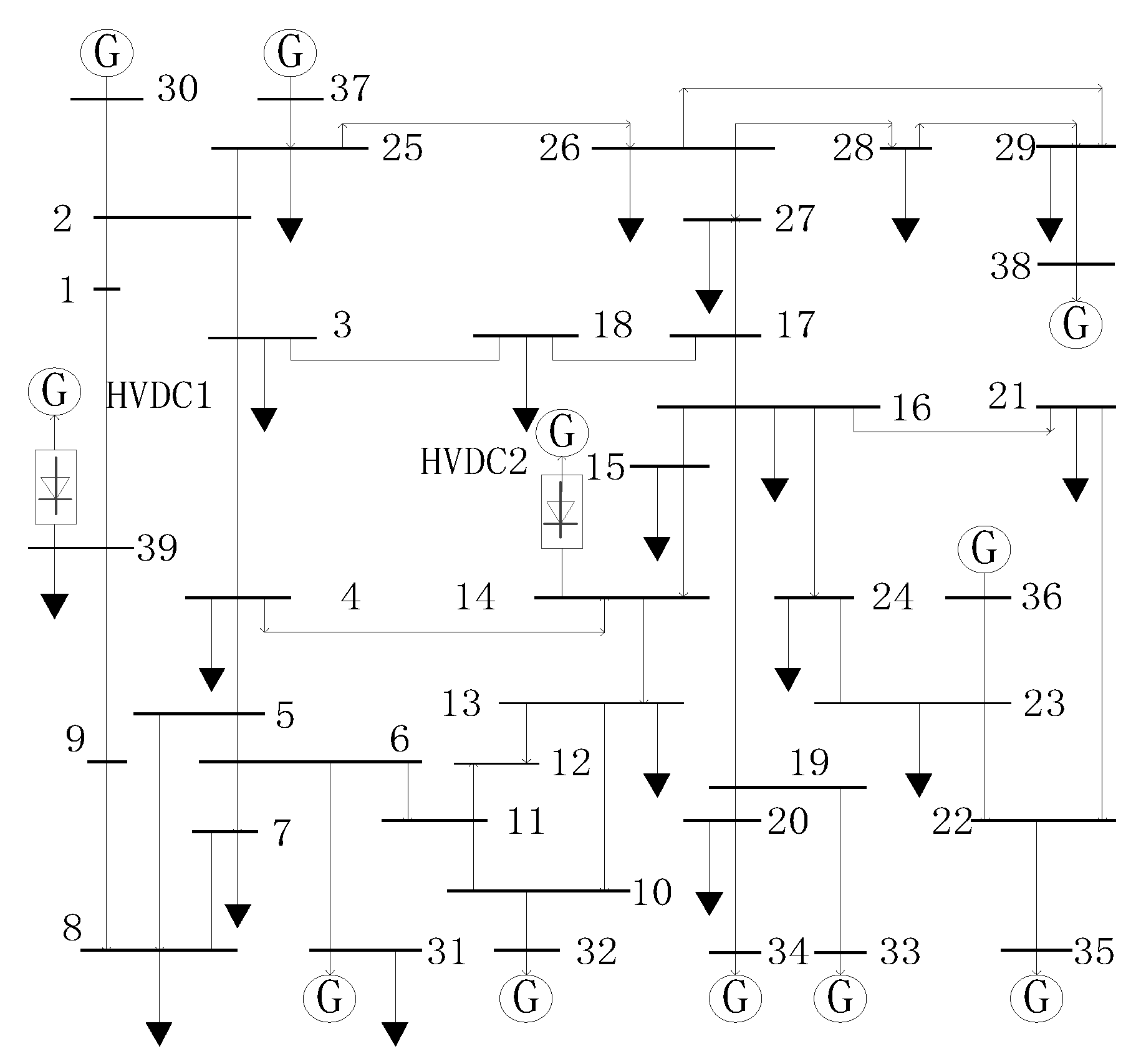
5.1. IEEE-39 Bus System

The modified IEEE-39 bus system, containing 9 generating and 2 HVDC transmission, is depicted in Figure 3. The rated capacity of two HVDCs are all 1000 MW, accounting for 29.4% of the total generator capacity 4800 MW. Data of generators and HVDC, and load, are shown in the supplementary. The following cases are considered to examine the efficiency of the proposed model. Then economic analysis, HVDC power consumption, frequency stability, and transmission power after HVDC blocking is analyzed.
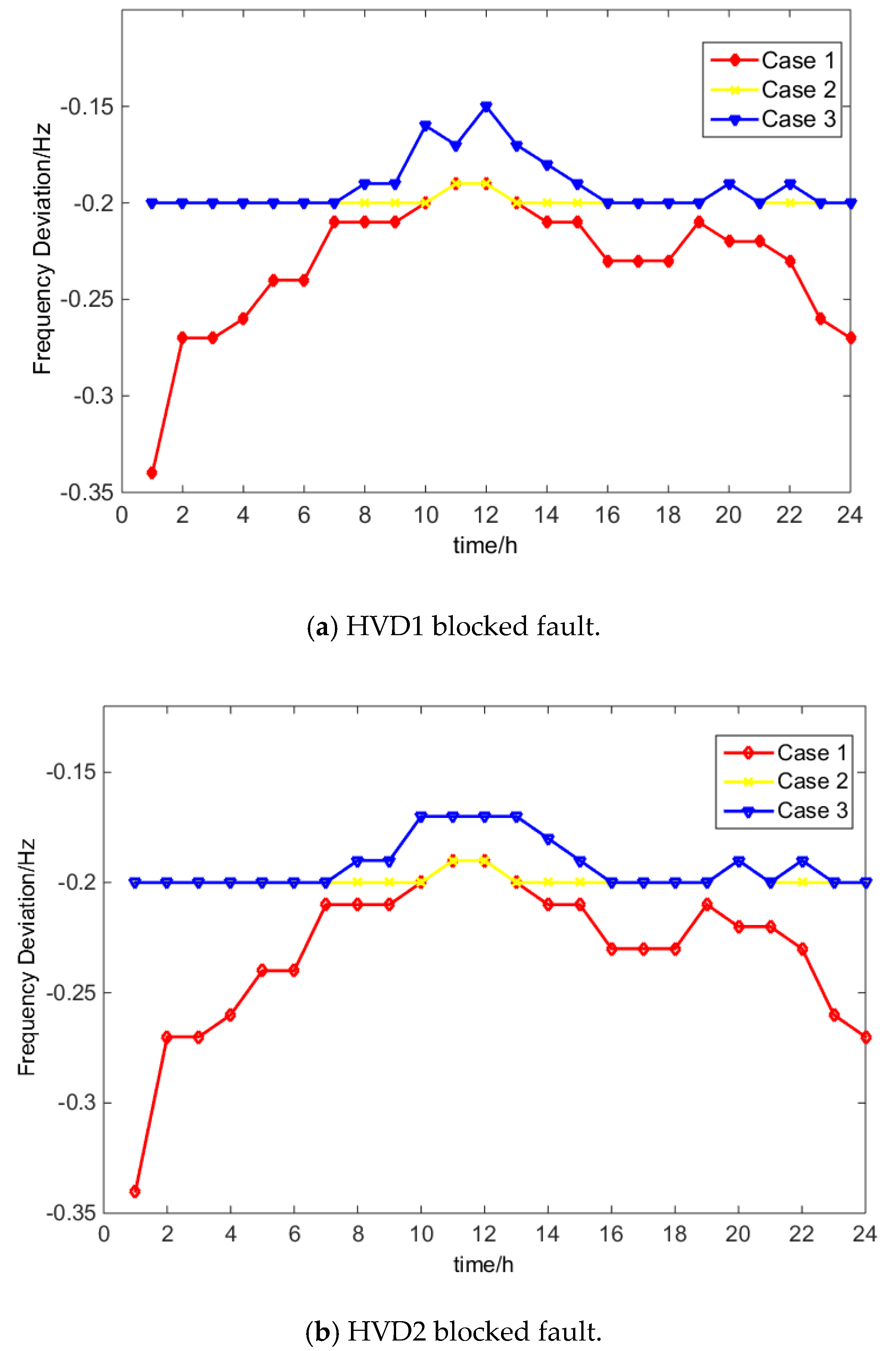
  • Case 0: UC solution with AC transmission constraints.
  • Case 1: SCUC solution with minimum frequency limits constraints.
  • Case 2: SCUC solution with minimum frequency limits constraints and security constraints after secondary frequency regulation.

5.1.1. Comparison of Economy and HVDC Consumption

The operating cost of three cases and average HVDC transmission power are shown in Table 1 and Figure 3. The concrete calculation results are shown in supplementary.
In case 0, HVDC operation cost is much lower than conventional units so that all two HVDCs are operated in rated capacity (1000 MW). In case 1, in order to ensure frequency deviation less than 0.2 Hz after one HVDC blocked, generating units start up while the HVDCs’ average power decreased to 989.2 MW. Although the total cost of case 1 is larger than case 1, the safety of the power system is already improved. In case 2, due to security constraints after the secondary frequency finished, two HVDCs’ average power continue to reduce to 967 MW and 974.9 MW, respectively. The safety of the power system would be further enhanced and the operational cost increase to $1,279,549, which is the highest of the three cases. From the perspective of computational efficiency, case 2 has the most calculation iterations, with 12 times and about 48 s.

5.1.2. Analysis of Frequency Stability

Based on the generators’ operation schedule in cases 0–2, after two HVDCs blocked separately, frequency deviation during simulation is shown in Figure 4.
In case 0, after HVDC 1 or 2 blocked, the frequency deviation is greater than 0.2 Hz except for hour 11 and 12, which cannot meet the requirement of the power system. The reason is that the two HVDCs are the operation of rated capacity so that less generators are turned on and the power system does not have enough reserve capacity. When the HVDC block happens, the frequency deviation drops under 49.8 Hz. In cases 1 and 2, the minimum frequency limit constraint is supplied into the model. It enforces more when the generator is turned on while the HVDC output decreases at the same time. As a result, more reserve capacity could be provided by generators and frequency deviation in all hours when they are within 0.2 Hz after HVDC 1 or 2 block. That is because the minimum frequency limits could raise the first frequency regulation capacity and improve the power grid’s reliability.

5.1.3. Analysis of Power Flow after HVDC Blocked

In consequence of security constraints, buses voltage and transmissions power operate within reasonable ranges in cases 1 and 2. When blocking failure happen to HVDC 1 or 2, secondary frequency regulation dispatch reserve capacity to compensate for real power gap. Then, the AC transmission power state is shown in Table 2 and Table 3.
According to Table 2, during hours 10–13, HVDC 1 in case 1 is rated power operation. After HVDC 1 blocked, transmission power between bus 9 and bus 39 is 389 MW, exceeding the rated capacity. However, this phenomenon would disappear in case 2 by introducing security constraints after secondary frequency regulation. The same situation also exists in transmission between bus 15 and 16 after HVDC 2 blocked in Table 3. It can be seen that the secondary frequency regulation could be able to deal with line power overload due to HVDC blocking failure.

5.2. Jiangsu Power Grid

As an important component of the eastern China power system, the Jiangsu power grid has put into operation two HVDCs in 2017, named Jinsu and Longzheng. It is a typical AC/DC hybrid receiving terminal power grid. Jinsu’s HVDC is fed into the Sunan district, which is the major load center in the Jiangsu power grid with weak reactive power support ability. Jiangsu power grid’s data of generators, HVDC, and load message are shown in the supplementary. To illuminate the effectiveness of the proposed method, two SCUC cases are built for the Jiangsu 500 kV power grid with 24 h:
Case 0:
SCUC solution with minimum frequency limits constraints and security constraints after secondary frequency regulation.
Case 1:
SCUC solution with minimum frequency limits constraints, security constraints after secondary frequency regulation and voltage stability constraints.
It is worth mentioning that the Jinsu HVDC is located in the Sunan district, which is the major load center in the Jiangsu power grid and has a shortage of reactive power support ability. Jinsu’s HVDC feed-in would cause generating units to shut down in this area so that the weaker voltage support capacity may further lead to a voltage stability problem. In this section, two UC cases are built for the Jiangsu 500 kV power grid within 24 h:
Forty-six generators in the Jiangsu 500 kV power grid provide a total capacity of 40,980 MW. The rated capacity of Jinsu and Longzheng are respectively 7200 MW and 3000 MW, accounting for 19.9% of the total installed generator capacity. Load data and the HVDC parameter are shown in the Appendix A.

5.2.1. Analysis of Voltage Stability of the Sunan Grid

Based on the optimal generator operation schedule of cases 0 and 1, static voltage stability of the Sunan grid with the Jinsu HVDC is analyzed. The results are shown in Table 4.
During load-peak hours such as hours 12 and 13, load of the Sunan grid is supplied by the Jinsu HVDC and external sources in case 0. As a result, less generators in the internal gird are turned ON and the static voltage stability margin is 7.6% and 7.8%, which is lower than the operation requirement of 8%. After minimum voltage stability constraints are added into case 1, relevant Benders cuts are generated and operation status of units in the Sunan grid are re-dispatched. As shown in Table 5, the static voltage stability margin would increase to 9.1% and 9.4% in hours 12 and 13, satisfying the operation requirement.

5.2.2. Analysis of Economy and HVDC Consumption

The operating costs and average HVDC power of both cases are shown in Table 5.
Compared with Longzheng’s HVDC full power operation in cases 0 and 1, the average power of Jinsu’s HVDC is 6539.4 MW and 5382.5 MW. The reason is that due to larger capacity, if Jinsu’s HVDC is full power operating, low frequency and overload of the transmission line problem will appear when Jinsu HVDC blocked. With relevant constraints of first and second frequency regulation capacity, Jinsu’s HVDC power is decreased at different levels. The difference of Jinsu’s HVDC power in cases 0 and 1 is caused by voltage stability constraints, explained in the last section. In addition, case 1 is has the most calculation iterations, 30 times and 189.6 s.

5.2.3. Analysis of Transmissions Power after HVDC Blocked

Based on the optimization results, transmissions power results after Jinsu’s HVDC blocked in all hours, are shown in Table 6.
In case 0, affected by the secondary frequency regulation of the power system, the Meli–Mudu double line is out of limit at some hours after Jinsu’s HVDC blocked; in case 1, by reducing Jinsu’s HVDC transmission power and optimizing the generators’ schedule, it ensures that the Meli–Mudu double lines still operates within limit after HVDC blocked.

6. Conclusions

The paper puts forward a UC model and algorithm for the AC/DC hybrid receiving end of the power grid. Considering voltage stability, low frequency, and transmission power overload after HVDC blocked, it respectively increases relevant constraints. We compared the proposed model with the conventional UC model by employing IEEE 39 and Jiangsu 500 kV power grid. The test results indicate that the algorithm is feasible and it can ensure the safety of the receiving end power grid.

Supplementary Materials

The following are available online at https://www.mdpi.com/2076-3417/9/16/3412/s1, Excel.

Author Contributions

Preparation of the manuscript was performed by N.Z., Q.Z. and H.H.

Funding

This research was funded by the State Grid Jiangsu Electric Power Co., LTD. Project of “Research on capacity confidence assessment and operating strategy of receive-end in AC/DC hybrid power grid with large-scale renewable energy power generation and energy storage system” (J2018096-2).

Acknowledgments

The authors gratefully acknowledge the support of the State Grid Project of “Research and demonstrative application on the technology of improving the voltage support capability of large-scale urban power grid.

Conflicts of Interest

The authors declare no conflict of interest.

Nomenclature

VdR, VdIDC voltage of rectifier/inverter
kR, kITransformer tap ratio of rectifier/inverter
γExtinguishing angle
Xc,R, Xc,ILeakage reactance of rectifier/inverter
RdResistance of HVDC line
QdR, QdIExchange reactive power between rectifier/inverter substation and AC grid
P d , l t , Q d , l t Real and reactive power of HVDC l at time t
lIndex of HVDC
m, nIndex of AC bus
NBNumber of buses
CsumThe total operation cost
u i t On/off state of generating unit i at time t
P L , m t , Q L , m t Real and reactive load of bus m at time t
r i t Reserve capacity of unit i at time t
P ¯ i , max , P _ i , min Upper and lower output limit considering ramp capacity of unit i
Q ¯ G , i , max / Q _ G , i , min Upper/lower reactive power limit of unit i
H S T i , C S T i Hot and cold start-up cost of unit i
T i , o n t , T i , o f f t Continuous on/off time of unit i at time t
U R i , D R i Ramp up and down capacity of unit i
Δ f max Maximal allowed frequency deviation
KLFirst frequency regulation coefficient of load
η V S M Voltage stability margin of power grid
P l 0 Initial real load of power grid
XmnLine reactance between bus m and n
P ¯ d t Maximum HVDC transmission power at time t
P l o s s t Real power loss of power grid at time t
V m , s t , V n , s t Voltage of AC bus m/n at time t after second frequency regulation
P L m n , s t Transmission power between bus m and n
MP1, MP2, MQ1, MQ2, MPL1, MPL2, MPD1, MPD2Mismatch vectors
ΔV, ΔθVector of units’ amplitude and phase increments
dP, dQMismatch vector of real and reactive power of AC buses
dPdc, dQdcMismatch vector of real and reactive power of HVDC
ΔPLVector of AC transmission power
H, N, J, L, W, S, O, D, E, FJacobian matrices
ΔQmin, ΔQmaxVector of units’ reactive power limits with increments
ΔVmin, ΔVmaxVector of voltage limits with increments
ΔXdc,min, ΔXdc,maxVector of dc variables limits with increments
ITmaxMaximum number of iteration
IdDC current
αTrigger delay angle
V m ( t ) , V n ( t ) Voltage of AC bus m/n (at time t)
n R , n I Bridge number of rectifier/inverter
PdR, PdIReal power of rectifier/inverter
QCR, QCIReactive power compensation of rectifier/inverter substation
iIndex of units
tIndex of hours
TNumber of scheduling periods
NLNumber of HVDC
CiCost function of unit i, Ci = ai( P G , i t )2 + bi P G , i t + ci
ai,bi,ciCoefficients of cost function
P G , i t , Q G , i t Real/reactive generation of unit i
P d , l t , Q d , l t Real and reactive power of DC l at time t
P ¯ G , i , max , P _ G , i , min Upper and lower real power limit of unit i
P L m n t Transmission power between bus m and n
S T i t Start up cost of unit i at time t
T i , u p , T i , d o w n Minimum continuous on/off time of unit i
T i , c o l d Cold start up time of unit i
P L m n , max , P L m n , min Transmission power limits between bus m and n
K G , i First frequency regulation coefficient of unit i
η min Minimum requirement of voltage stability margin
P l * Ultimate real load of power grid
Gmn, BmnAdmittance between bus m and n
θ m n t Phase difference between bus m and n at time t
P L , s u m t Total load of power grid at time t
Δ P G , i , s t , Δ Q G , i , s t Real/reactive power increment of unit i after second frequency regulation
θ m n , s t Voltage phase difference between bus m and n at time t after second frequency regulation
wtObjective of sub-model
() *Optimization result of the last iteration
ΔPG, ΔQGVector of units’ real and reactive power increments
ΔPdc, ΔQdcVector of units’ real and reactive power increments
ΔXac, ΔXdcVector of AC/DC variables
dPLMismatch vector of transmission power
  λ ,   ψ _ , ψ ¯   Simplex multipliers
ΔPLmin, ΔPLmaxVector of transmissions power limits with increments
ΔXac,min, ΔXac,maxVector of AC variables limits with increments

Appendix A

A Sub-model of the second frequency regulation is shown as following:
M i n w t = ( M P L 1 + M P L 2 )
[ Δ P G Δ Q G ] + [ H N J L ] [ Δ θ Δ V ] + [ Δ P d c Δ Q d c ] + [ M P 1 M Q 1 ] [ M P 2 M Q 2 ] = [ d P d Q ]
[ Δ P d c Δ Q d c ] + [ O D E F ] [ Δ X a c Δ X d c ] + [ M P 1 D M Q D 1 ] [ M P D 2 M Q D 2 ] = [ d P d c d Q d c ]
Δ P L + [ Z S ] [ Δ θ Δ V ] + M P L 1 M P L 2 = d P L
Δ P G = 0        λ
Δ P d c = 0
0 < M P i , 1 < r i t
0 < M P i , 2 < r i t
Δ Q min Δ Q Δ Q max ψ _ , ψ ¯
Δ P L min Δ P L Δ P L max
Δ V min Δ V Δ V max
Δ X a c , min Δ X a c Δ X a c , max
Δ X d c , min Δ X d c Δ X d c , max

References

  1. Bin, W.; Ye, X.; Qing, X. Wind power integrated dynamic optimal power flow for AC/DC interconnected system. Autom. Electr. Power Syst. 2016, 40, 34–41. [Google Scholar]
  2. Hongwei, H.; Mengfu, T.; Huiling, Z. Day-ahead generation scheduling method considering adjustable HVDC plan and its analysis. Autom. Electr. Power Syst. 2015, 39, 138–142. [Google Scholar]
  3. Lotfjou, A.; Shahidehpour, M.; Fu, Y. Hourly scheduling of DC transmission lines in SCUC with voltage source converters. IEEE Trans. Power Syst. 2011, 26, 650–660. [Google Scholar] [CrossRef]
  4. Wydra, M. Performance and Accuracy Investigation of the Two-Step Algorithm for Power System State and Line Temperature Estimation. Energies 2018, 11, 1005. [Google Scholar] [CrossRef]
  5. Wydra, M.; Kubaczynski, P.; Mazur, K.; Ksiezopolski, B. Time-Aware Monitoring of Overhead Transmission Line Sag and Temperature with LoRa Communication. Energies 2019, 12, 505. [Google Scholar] [CrossRef]
  6. Mazur, K.; Wydra, M.; Ksiezopolski, B. Secure and Time-Aware Communication of Wireless Sensors Monitoring Overhead Transmission Lines. Sensors 2017, 17, 1610. [Google Scholar] [CrossRef] [PubMed]
  7. Sampath, L.; Hotz, M.; Gooi, H.B.; Utschick, W. Unit commitment with AC power flow constraints for a hybrid transmission grid. In Proceedings of the 20th Power Systems Computation Conference, Dublin, Ireland, 11–15 June 2018. [Google Scholar]
  8. Mesanovic, A.; Munz, U.; Ebenbauer, C. Robust optimal power flow for mixed AC/DC transmission systems with volatile renewables. IEEE Trans. Power Syst. 2018, 33, 5171–5182. [Google Scholar] [CrossRef]
  9. Bin, W.; Ye, X.; Qing, X. Security-Constrained economic dispatch with AC/DC interconnection system based on Benders decomposition method. Proc. CSEE 2016, 36, 1588–1595. [Google Scholar]
  10. Lotfjou, A.; Shahidehpour, M.; Fu, Y.; Li, Z. Security-constrained unit commitment with AC/DC transmission systems. IEEE Trans. Power Syst. 2010, 25, 531–542. [Google Scholar] [CrossRef]
  11. Wang, B.; Xia, Y.; Zhong, H. Coordinated optimization of unit commitment and DC transmission power scheduling using Benders decomposition. DRPT 2015, 648–653. [Google Scholar] [CrossRef]
  12. Zhou, M.; Zhai, J.; Li, G.; Ren, J. Distributed dispatch approach for bulk AC/DC hybrid systems with high wind power penetration. IEEE Trans. Power Syst. 2018, 33, 3325–3336. [Google Scholar] [CrossRef]
  13. Xie, K.; Dong, J.; Tai, He. Optimal planning of HVDC-based bundled wind-thermal generation and transmission system. Energy Convers. Manag. 2016, 115, 71–79. [Google Scholar] [CrossRef]
  14. Hajeforosh, S.F.; Pooranian, Z.; Shabani, A.; Conti, M. Evaluating the High Frequency Behavior of the Modified Grounding Scheme in Wind Farms. Appl. Sci. 2017, 7, 1323. [Google Scholar] [CrossRef]
  15. Donglei, S.; Xueshan, H.; Jinhong, Y. Power system unit commitment considering voltage regulation effect. Trans. China Electrotech. Soc. 2016, 31, 107–117. [Google Scholar]
  16. Miguel, C.; Jose, M.A. A computationally efficient mixed-integer linear formulation for the thermal unit commitment problem. IEEE Trans. Power Syst. 2006, 21, 1371–1378. [Google Scholar]
  17. Yong, F.; Mohammad, S.; Zuyi, L. Security-constrained unit commitment with AC constraints. IEEE Trans. Power Syst. 2005, 20, 1538–1550. [Google Scholar]
Figure 1. Diagram of HVDC system.
Applsci 09 03412 g001
Figure 2. The flow chart of solving the proposed UC model.
Applsci 09 03412 g002
Figure 3. The diagram of reformed IEEE 39-bus system.
Applsci 09 03412 g003
Figure 4. Frequency deviation after HVDC 1 and 2 blocked fault.
Applsci 09 03412 g004
Table 1. Operating cost and HVDC power.
Cost/$HVDC 1′s Average Power/MWHVDC 2′s Average Power/MWIteration TimesComputing Time/s
Case 01,157,6771000.01000.0115.0
Case 11,229,612989.2989.2731.6
Case 21,279,549967.0974.91248.0
Table 2. HVDC 1 transmission power and AC transmission power HVDC1 block fault.
Case 1Case 2
HVDC 1′s PowerLines’ Over LimitsHVDC 1′s PowerLines’ Over Limits
Hour 101000Power between bus-9 and bus-39 is 393.9 MW956.0--
Hour 111000Power between bus-9 and bus-39 is 390.7 MW1000--
Hour 121000Power between bus-9 and bus-39 is 404.2 MW873.7--
Hour 131000Power between bus-9 and bus-39 is 398.7 MW981.4--
Table 3. HVDC 2 transmission power and AC transmission power HVDC1 block fault.
Case 1Case 2
HVDC 2′s PowerLine Power’s OverloadHVDC 2′s PowerLine Power’s Overload
Hour 71000Power between bus-16 and bus-15 is 505.9 MW1000--
Hour 8989.5Power between bus-16 and bus-15 is 535.0 MW1000--
Hour 15985.6Power between bus-16 and bus-15 is 540.7 MW1000--
Hour 19980.4Power between bus-16 and bus-15 is 520.6 MW989.5--
Hour 211000Power between bus-16 and bus-15 is 505.3 MW989.5--
Table 4. Static voltage stability margin of the Sunan grid with the JINSU HVDC fed-in.
Case 1Case 2
Active Load/MWStatic Voltage Stability MarginActive Load/MWStatic Voltage Stability Margin
Hour 1232,0007.6%32,0009.1%
Hour 1331,7007.8%31,7009.4%
Table 5. Operating cost and HVDC power.
Cost/$Longzheng HVDC’s Average Power/MWJinsu HVDC’s Average Power/MWIteration TimesComputing Time/s
Case 09,695,35130006539.41170.7
Case110,691,68330005382.530189.6
Table 6. Jinsu power and operation of branches after Jinsu block fault.
Case 1Case 2
Jinsu HVDC’s PowerLine Power’s OverloadJinsu HVDC’s PowerLine Power’s Overload
Hour 66628Power between Meili and Mudu is 2040 MW2633--
Hour 76664Power between Meili and Mudu is 2040 MW2671--
Hour 86691Power between Meili and Mudu is 2166 MW2785--
Hour 96700Power between Meili and Mudu is 2144 MW2956--
Hour 156678Power between Meili and Mudu is 2177 MW3098--
Hour 166610Power between Meili and Mudu is 2067 MW2649--
Addition: Power limit of Meili and Mudu is 2000 MW.

