Multiple Convolutional Neural Networks Fusion Using Improved Fuzzy Integral for Facial Emotion Recognition


Abstract
:1. Introduction
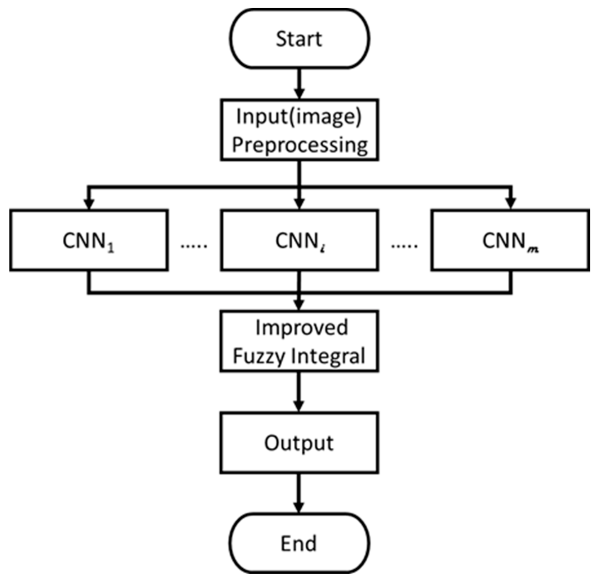
2. Proposed MCNNs-IFI
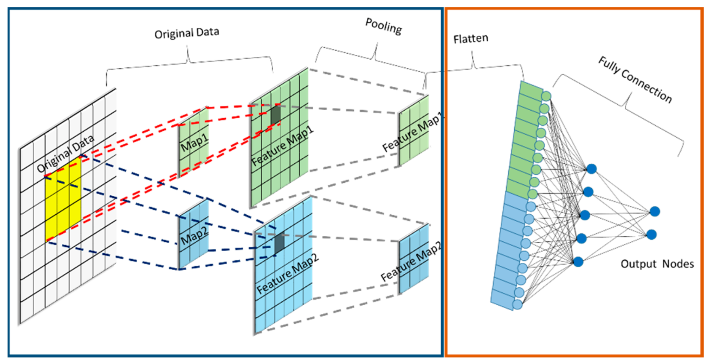
2.1. CNN
2.1.1. Convolution Layer
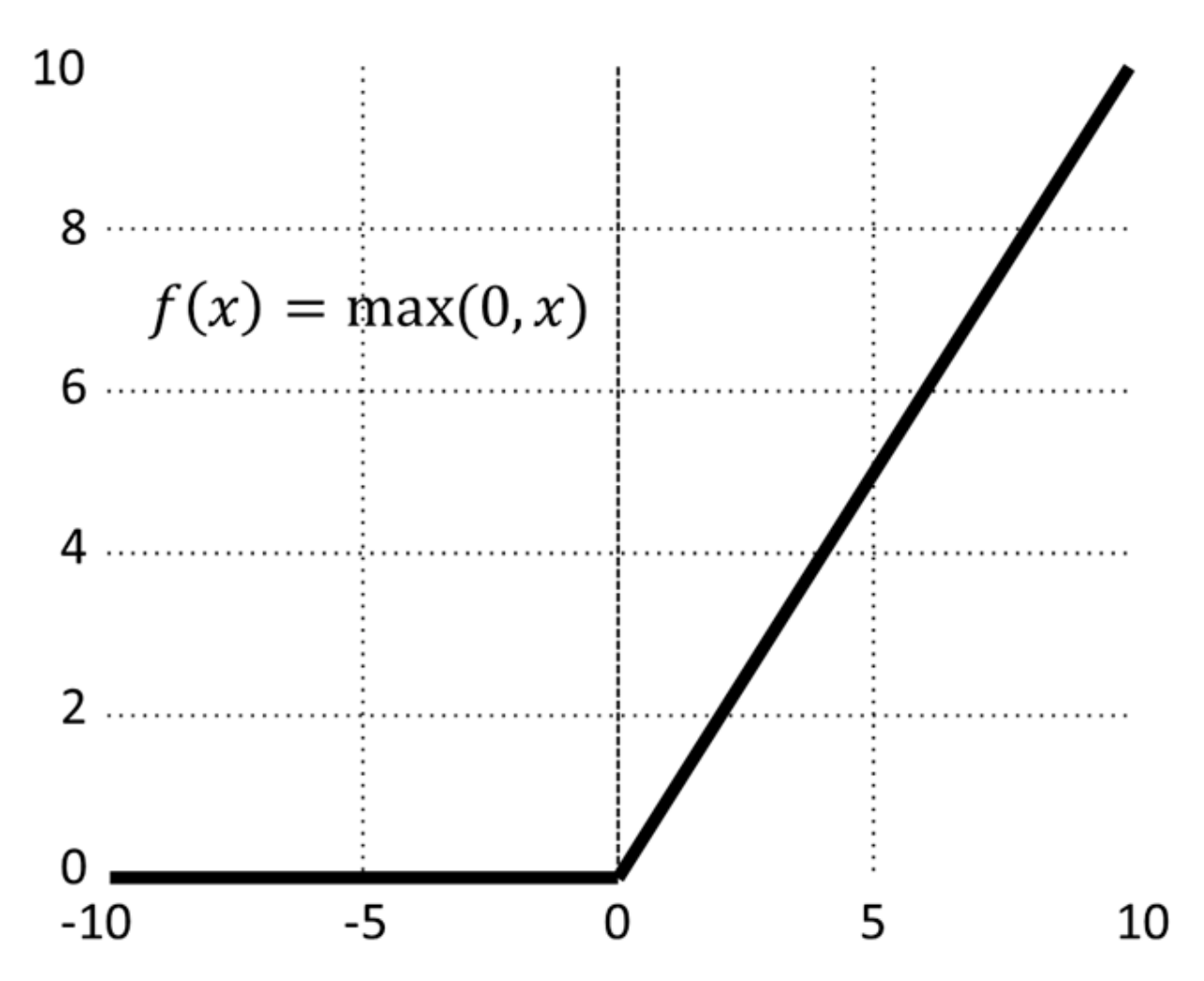
2.1.2. Activation Function
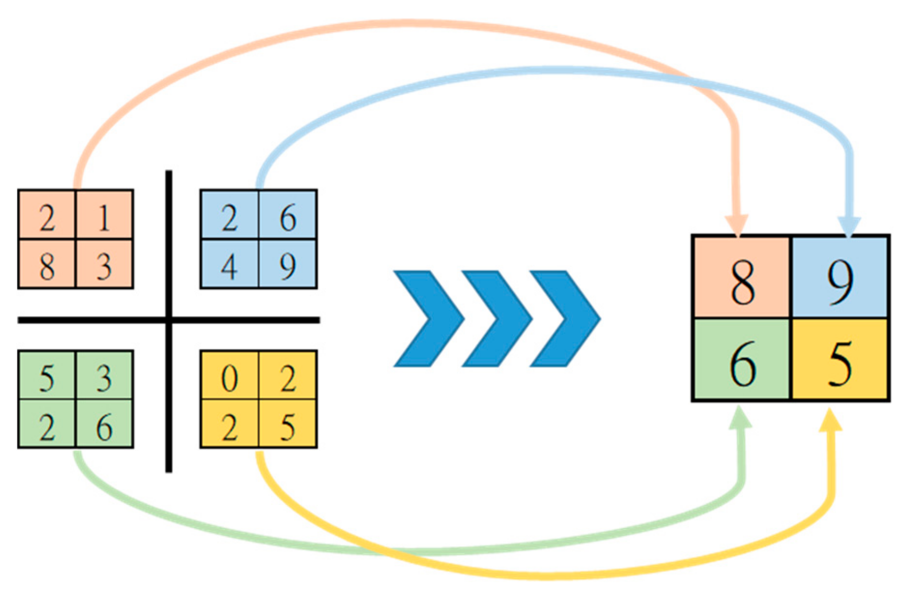
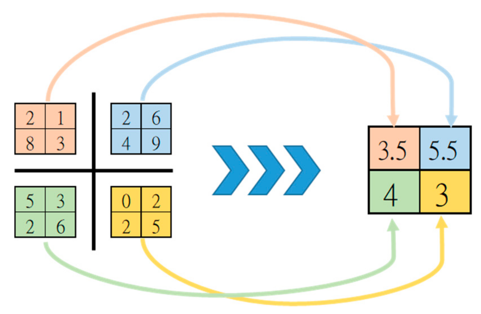
2.1.3. Pooling Layer
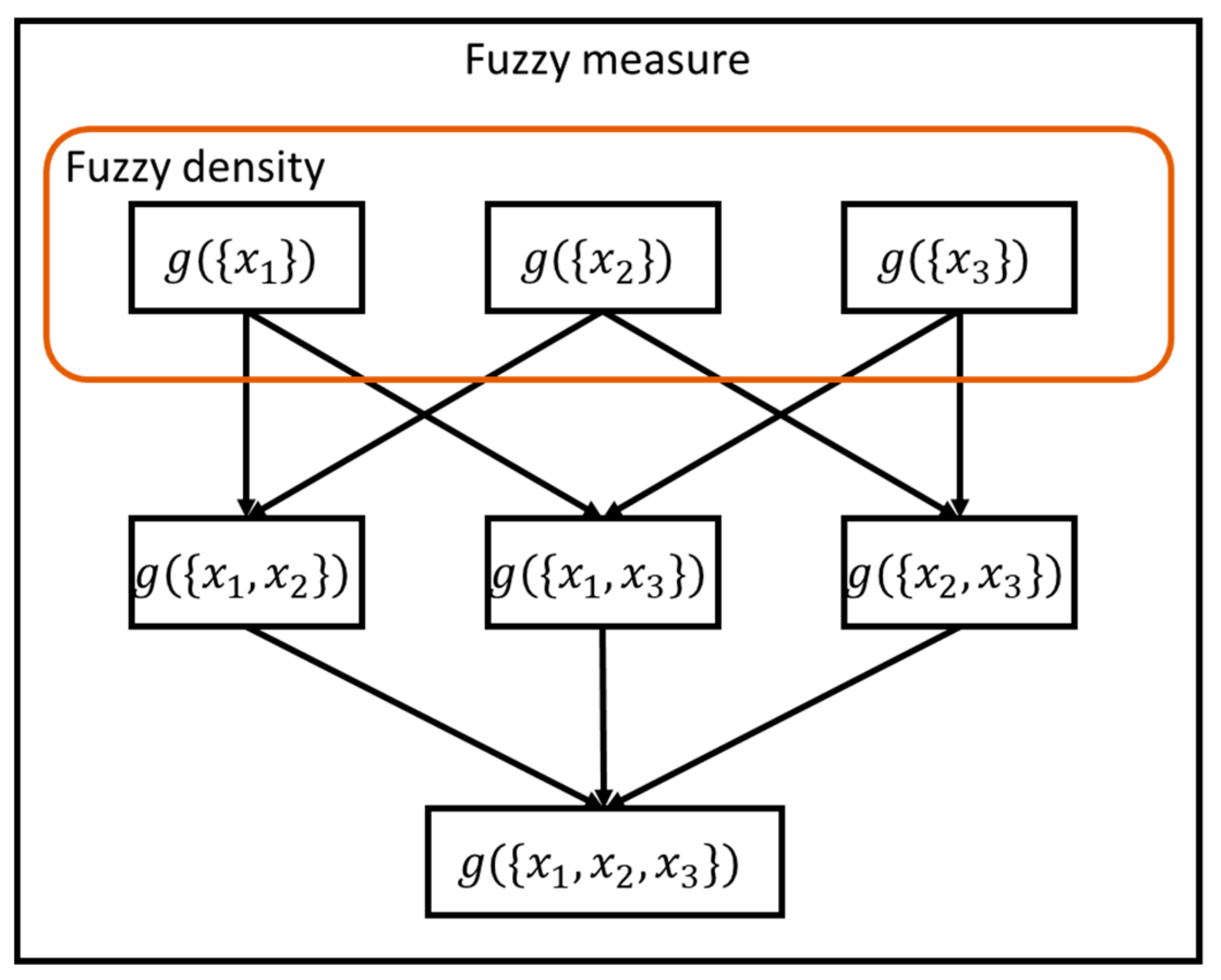
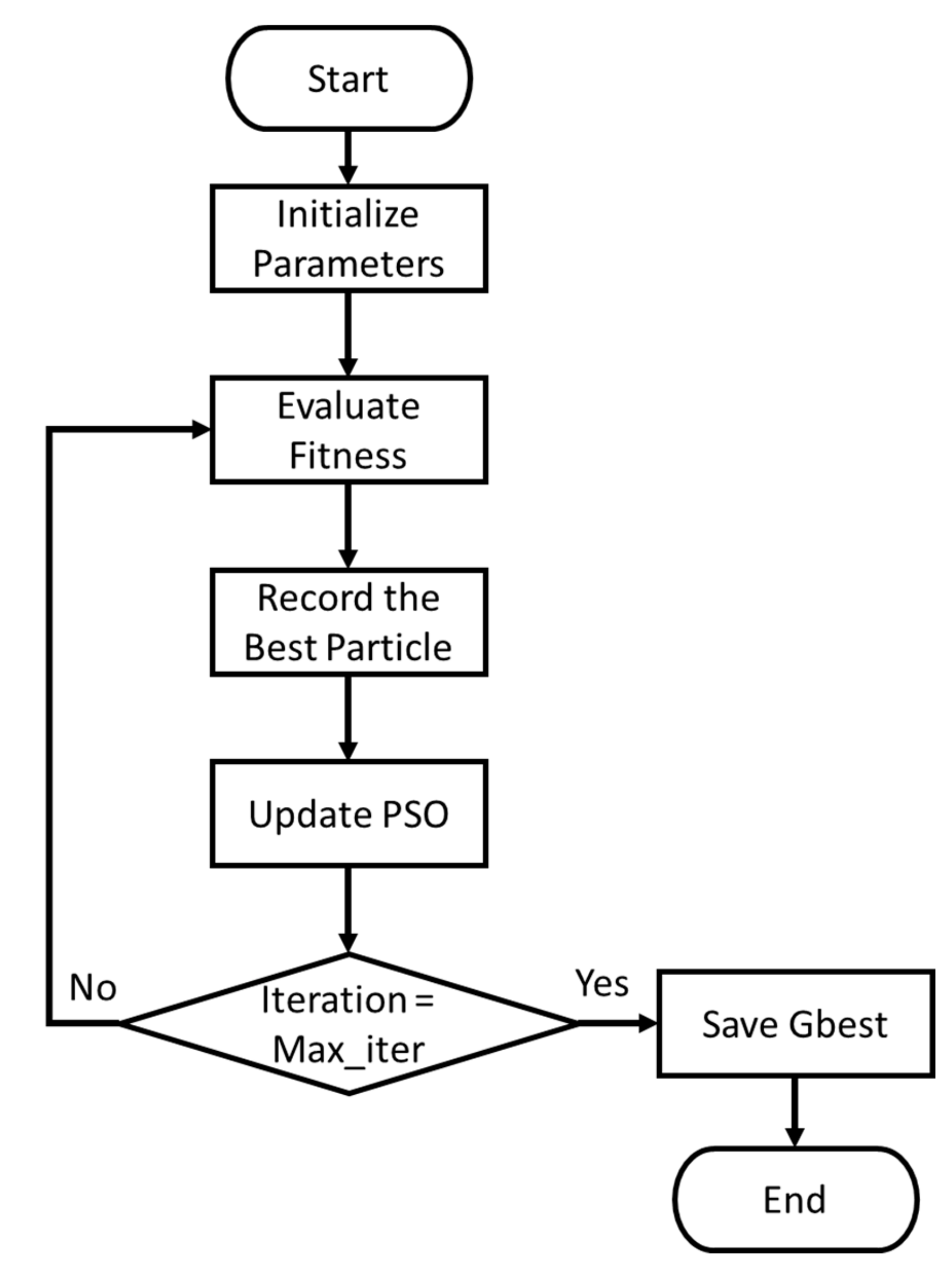
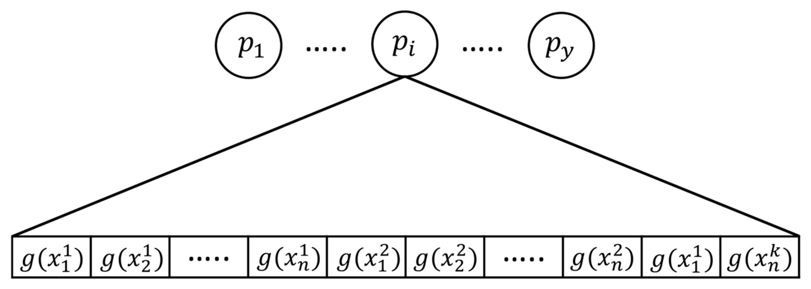
2.2. Proposed Improved Fuzzy Integral
- (1)
- g(X) = 1 indicates that when all classifier outputs are consistent, the results must be trusted.
- (2)
- g(∅) = 0 indicates that outputs of all classifiers are not considered.
- (3)
- Fuzzy measure should be an incremental monotonic function:
- (1)
- (2)
- (3)
3. Experimental Results
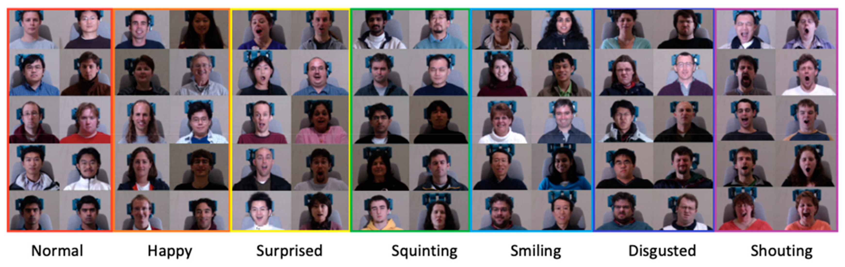
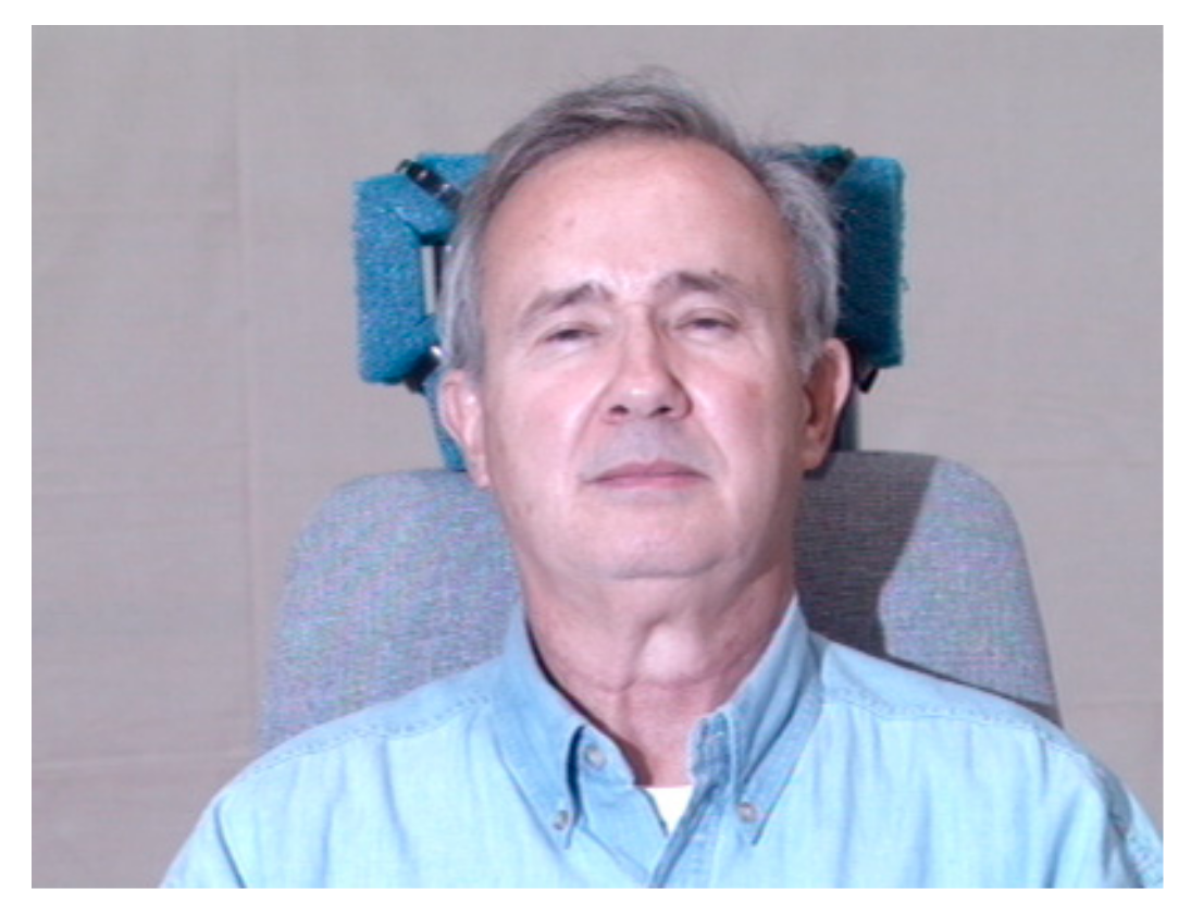
3.1. Multi-PIE Face Database
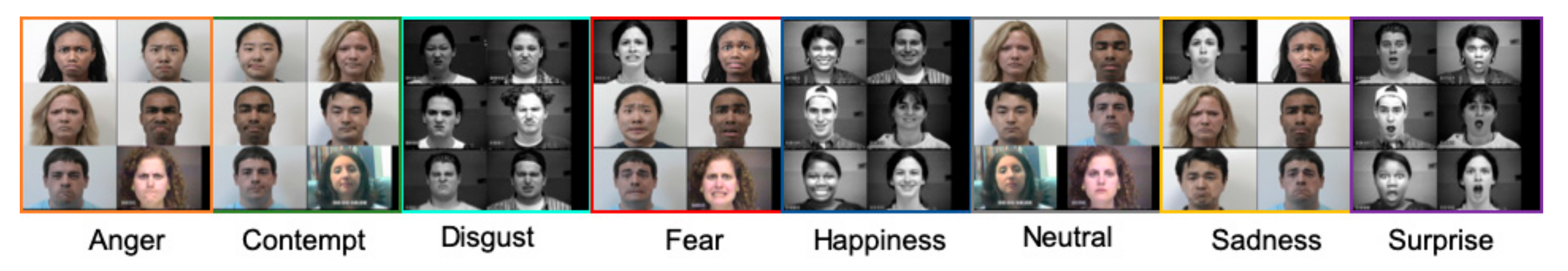
3.2. CK+ Database
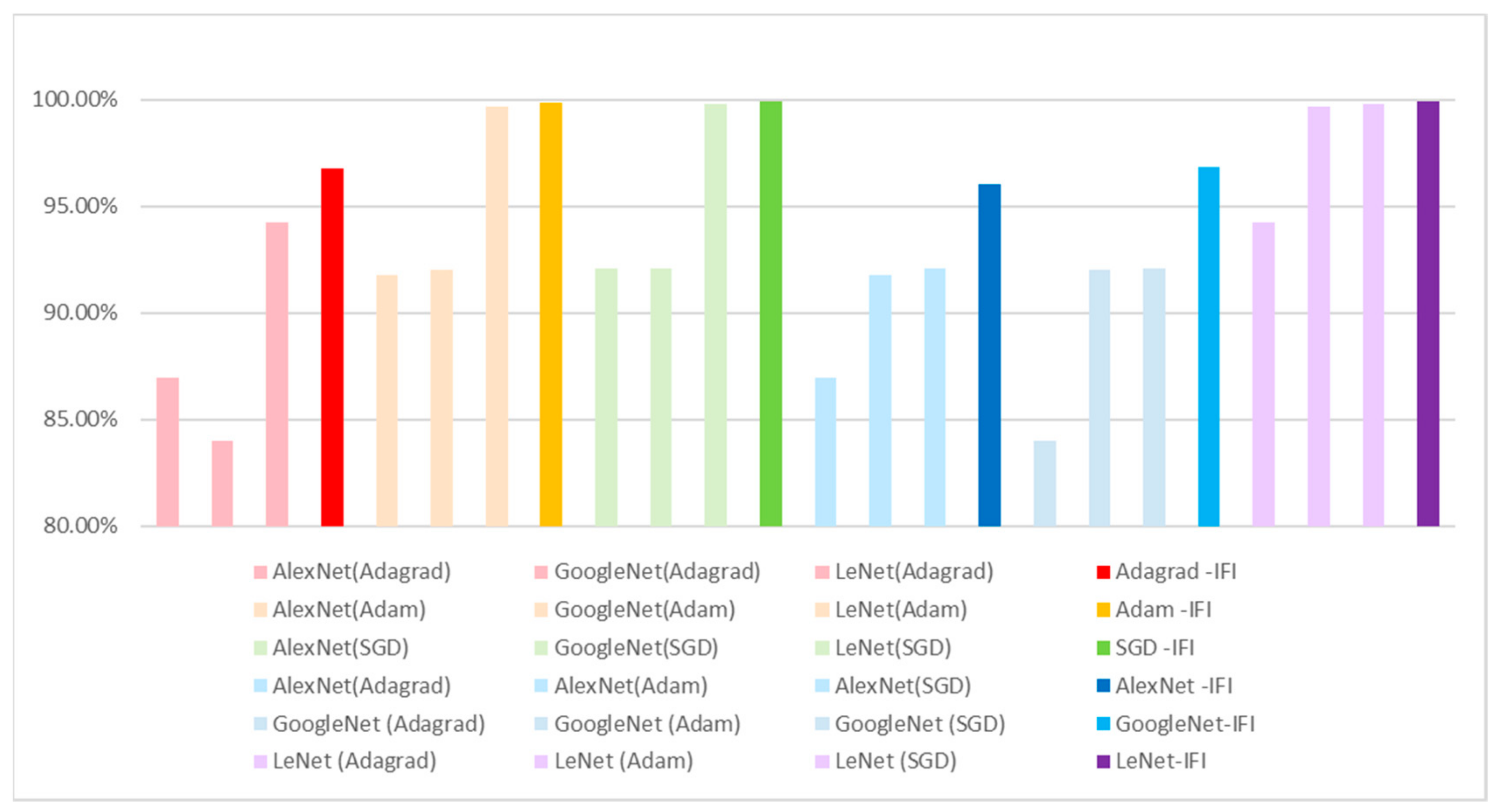
3.3. Discussion
4. Conclusions
Author Contributions
Funding
Conflicts of Interest
References
- LeCun, Y.; Bottou, L.; Bengio, Y.; Haffner, P. Gradient-based learning applied to document recognition. Proc. IEEE 1998, 86, 2278–2323. [Google Scholar] [CrossRef]
- Rumelhart, E.; Hinton, E.; Williams, J. Learning representations by back-propagating errors. Nature 1986, 323, 533–536. [Google Scholar] [CrossRef]
- Szegedy, C.; Liu, W.; Jia, Y.; Sermanet, P.; Reed, S.; Anguelov, D.; Erhan, D.; Vanhoucke, V.; Rabinovich, A. Going deeper with convolutions. In Proceedings of the IEEE Conference on Computer Vision and Pattern Recognition, Boston, MA, USA, 7–12 June 2015; pp. 1–9. [Google Scholar]
- Krizhevsky, A.; Sutskever, I.; Hinton, G.E. ImageNet classification with deep convolutional neural networks. In Proceedings of the 25th International Conference on Neural Information Processing Systems (NIPS’12), Lake Tahoe, NV, USA, 3–6 December 2012; Volume 1, pp. 1097–1105. [Google Scholar]
- Liu, S.; Deng, W. Very Deep convolutional neural network based image classification using small training sample size. In Proceedings of the 2015 3rd IAPR Asian Conference on Pattern Recognition (ACPR), Kuala Lumpur, Malaysia, 3–6 November 2015; pp. 730–734. [Google Scholar]
- Ioffe, S.; Szegedy, C. Batch normalization: Accelerating deep network training by reducing internal covariate shift. In Proceedings of the 32nd International Conference on Machine Learning, Lille, France, 6–11 July 2015; Volume 37, pp. 448–456. [Google Scholar]
- Wu, S.; Zhong, S.; Liu, Y. Deep residual learning for image steganalysis. Multimed. Tools Appl. 2018, 77, 10437–10453. [Google Scholar] [CrossRef]
- Lin, M.; Chen, Q.; Yan, S. Network in network. In Proceedings of the International Conference on Learning Representations (ICLR), Scottsdale, AZ, USA, 2–4 May 2013; pp. 1–10. [Google Scholar]
- Asness, C.S.; Moskowitz, T.J.; Pedersen, L.H. Value and momentum everywhere. J. Financ. 2013, 68, 929–985. [Google Scholar] [CrossRef]
- Duchi, J.; Hazan, E.; Singer, Y. Adaptive subgradient methods for online learning and stochastic optimization. J. Mach. Learn. Res. 2011, 12, 2121–2159. [Google Scholar]
- Ruder, S. An overview of gradient descent optimization algorithms. arXiv 2017, arXiv:1609.04747, 1–14. [Google Scholar]
- Kingma, D.P.; Ba, J. Adam: A method for stochastic optimization. In Proceedings of the 3rd International Conference for Learning Representations, San Diego, CA, USA, 7–9 May 2015; pp. 1–15. [Google Scholar]
- Soto, V.; Suárez, A.; Martínez-Muñoz, G. An urn model for majority voting in classification ensembles. In Proceedings of the 30th Conference on Neural Information Processing Systems (NIPS 2016), Barcelona, Spain, 5–10 December 2016; pp. 1–9. [Google Scholar]
- Kuncheva, L.I. Combining classifiers: Soft computing solutions. In Pattern Recognition, From Classical to Modern Approaches; Pal, S.K., Pal, A., Eds.; World Scientific: Singapore, 2001; Volume 15, pp. 427–452. [Google Scholar]
- Kevric, J.; Jukic, S.; Subasi, A. An effective combining classifier approach using tree algorithms for network intrusion detection. Neural Comput. Appl. 2017, 28 (Suppl. 1), 1051–1058. [Google Scholar] [CrossRef]
- Lin, C.J.; Kuo, S.S.; Peng, C.C. Multiple functional neural fuzzy networks fusion using fuzzy integral. Int. J. Fuzzy Syst. 2012, 14, 380–391. [Google Scholar]
- Zhang, Y.; Li, H.G.; Wang, Q. A filter-based bare-bone particle swarm optimization algorithm for unsupervised feature selection. Appl. Intell. 2019, 1–10. [Google Scholar] [CrossRef]


| 10-folder CV | AlexNet (Adagrad) | GoogleNet (Adagrad) | LeNet (Adagrad) | AlexNet(Adagrad) + GoogleNet(Adagrad) + LeNet(Adagrad) + IFI |
|---|---|---|---|---|
| Round 1 | 85.82% | 84.25% | 90.75% | 96.18% |
| Round 2 | 88.14% | 87.11% | 96.54% | 97.75% |
| Round 3 | 84.71% | 83.89% | 98.71% | 98.76% |
| Round 4 | 85.54% | 82.71% | 98.32% | 98.43% |
| Round 5 | 87.25% | 84.25% | 93.61% | 97.46% |
| Round 6 | 93.57% | 84.68% | 97.50% | 98.89% |
| Round 7 | 87.18% | 78.39% | 95.11% | 97.11% |
| Round 8 | 84.18% | 84.57% | 84.18% | 91.61% |
| Round 9 | 85.36% | 82.61% | 93.96% | 95.71% |
| Round 10 | 87.50% | 87.57% | 93.93% | 97.07% |
| Average | 86.93% | 84.00% | 94.26% | 96.79% |
| 10-folder CV | AlexNet (Adam) | GoogleNet (Adam) | LeNet (Adam) | AlexNet(Adam) + GoogleNet(Adam) + LeNet(Adam) + IFI |
|---|---|---|---|---|
| Round 1 | 92.00% | 86.00% | 99.00% | 100.00% |
| Round 2 | 92.21% | 90.85% | 99.64% | 99.79% |
| Round 3 | 89.92% | 93.25% | 99.89% | 99.89% |
| Round 4 | 92.21% | 92.25% | 99.75% | 99.78% |
| Round 5 | 92.60% | 93.60% | 99.75% | 99.92% |
| Round 6 | 92.60% | 92.32% | 99.71% | 99.78% |
| Round 7 | 91.42% | 94.00% | 99.67% | 99.82% |
| Round 8 | 92.00% | 94.53% | 99.82% | 99.85% |
| Round 9 | 91.03% | 91.42% | 99.67% | 99.78% |
| Round 10 | 91.67% | 91.67% | 99.96% | 99.96% |
| Average | 91.77% | 91.99% | 99.69% | 99.85% |
| 10-folder CV | AlexNet (SGD) | GoogleNet (SGD) | LeNet (SGD) | AlexNet(SGD) + GoogleNet(SGD) + LeNet(SGD) + IFI |
|---|---|---|---|---|
| Round 1 | 90.79% | 93.53% | 99.96% | 99.96% |
| Round 2 | 93.21% | 93.57% | 99.86% | 99.95% |
| Round 3 | 92.53% | 93.75% | 99.89% | 99.91% |
| Round 4 | 91.00% | 91.32% | 99.79% | 99.91% |
| Round 5 | 92.36% | 85.07% | 99.71% | 99.89% |
| Round 6 | 93.25% | 94.42% | 99.64% | 99.96% |
| Round 7 | 91.75% | 92.18% | 99.82% | 99.90% |
| Round 8 | 91.46% | 91.07% | 99.75% | 99.89% |
| Round 9 | 93.06% | 95.32% | 99.64% | 99.97% |
| Round 10 | 91.36% | 90.71% | 99.82% | 99.96% |
| Average | 92.08% | 92.09% | 99.79% | 99.93% |
| 10-folder CV | AlexNet (Adagrad) | AlexNet (Adam) | AlexNet (SGD) | AlexNet(Adagrad + Adam + SGD) + IFI |
|---|---|---|---|---|
| Round 1 | 85.82% | 92.00% | 90.79% | 94.21% |
| Round 2 | 88.14% | 92.21% | 93.21% | 95.89% |
| Round 3 | 84.71% | 89.92% | 92.53% | 96.79% |
| Round 4 | 85.54% | 92.21% | 91.00% | 95.89% |
| Round 5 | 87.25% | 92.60% | 92.36% | 96.43% |
| Round 6 | 93.57% | 92.60% | 93.25% | 97.21% |
| Round 7 | 87.18% | 91.42% | 91.75% | 96.07% |
| Round 8 | 84.18% | 92.00% | 91.46% | 95.93% |
| Round 9 | 85.36% | 91.03% | 93.06% | 96.14% |
| Round 10 | 87.50% | 91.67% | 91.36% | 95.96% |
| Average | 86.93% | 91.77% | 92.08% | 96.05% |
| 10-folder CV | GoogleNet (Adagrad) | GoogleNet (Adam) | GoogleNet (SGD) | GoogleNet (Adagrad + Adam + SGD) + IFI |
|---|---|---|---|---|
| Round 1 | 84.25% | 86.00% | 93.53% | 96.96% |
| Round 2 | 87.11% | 90.85% | 93.57% | 97.21% |
| Round 3 | 83.89% | 93.25% | 93.75% | 97.07% |
| Round 4 | 82.71% | 92.25% | 91.32% | 96.14% |
| Round 5 | 84.25% | 93.60% | 85.07% | 96.25% |
| Round 6 | 84.68% | 92.32% | 94.42% | 97.18% |
| Round 7 | 78.39% | 94.00% | 92.18% | 97.64% |
| Round 8 | 84.57% | 94.53% | 91.07% | 96.25% |
| Round 9 | 82.61% | 91.42% | 95.32% | 97.68% |
| Round 10 | 87.57% | 91.67% | 90.71% | 95.96% |
| Average | 84.00% | 91.99% | 92.09% | 96.84% |
| 10-folder CV | LeNet (Adagrad) | LeNet (Adam) | LeNet (SGD) | LeNet (Adagrad + Adam + SGD) + IFI |
|---|---|---|---|---|
| Round 1 | 90.75% | 99.00% | 99.96% | 100.00% |
| Round 2 | 96.54% | 99.64% | 99.86% | 99.89% |
| Round 3 | 98.71% | 99.89% | 99.89% | 99.97% |
| Round 4 | 98.32% | 99.75% | 99.79% | 99.93% |
| Round 5 | 93.61% | 99.75% | 99.71% | 99.84% |
| Round 6 | 97.50% | 99.71% | 99.64% | 99.82% |
| Round 7 | 95.11% | 99.67% | 99.82% | 99.83% |
| Round 8 | 84.18% | 99.82% | 99.75% | 99.85% |
| Round 9 | 93.96% | 99.67% | 99.64% | 99.96% |
| Round 10 | 93.93% | 99.96% | 99.82% | 100.00% |
| Average | 94.26% | 99.69% | 99.79% | 99.90% |
| Methods | AlexNet (Adagrad) | GoogleNet (Adagrad) | LeNet (Adagrad) | AlexNet(Adagrad) + GoogleNet(Adagrad) + LeNet(Adagrad) + IFI |
|---|---|---|---|---|
| Accuracy | 83.33% | 88.07% | 97.69% | 97.94% |
| Methods | AlexNet (Adam) | GoogleNet (Adam) | LeNet (Adam) | AlexNet(Adam) + GoogleNet(Adam) + LeNet(Adam) + IFI |
|---|---|---|---|---|
| Accuracy | 93.97% | 91.92% | 97.3% | 98.58% |
| Methods | AlexNet (SGD) | GoogleNet (SGD) | LeNet (SGD) | AlexNet(SGD) + GoogleNet(SGD) + LeNet(SGD) + IFI |
|---|---|---|---|---|
| Accuracy | 90.89% | 91.41% | 97.43% | 97.94% |
| Methods | AlexNet (Adagrad) | AlexNet (Adam) | AlexNet (SGD) | AlexNet(Adagrad + Adam + SGD) + IFI |
|---|---|---|---|---|
| Accuracy | 83.33% | 93.97% | 90.89% | 95.76% |
| Methods | GoogleNet (Adagrad) | GoogleNet (Adam) | GoogleNet (SGD) | GoogleNet (Adagrad + Adam + SGD) + IFI |
|---|---|---|---|---|
| Accuracy | 88.07% | 91.92% | 91.41% | 96.92% |
| Methods | LeNet (Adagrad) | LeNet (Adam) | LeNet (SGD) | LeNet (Adagrad + Adam + SGD) + IFI |
|---|---|---|---|---|
| Accuracy | 97.69% | 97.3% | 97.43% | 98.07% |
© 2019 by the authors. Licensee MDPI, Basel, Switzerland. This article is an open access article distributed under the terms and conditions of the Creative Commons Attribution (CC BY) license (http://creativecommons.org/licenses/by/4.0/).
Share and Cite
Lin, C.-J.; Lin, C.-H.; Wang, S.-H.; Wu, C.-H. Multiple Convolutional Neural Networks Fusion Using Improved Fuzzy Integral for Facial Emotion Recognition. Appl. Sci. 2019, 9, 2593. https://doi.org/10.3390/app9132593
Lin C-J, Lin C-H, Wang S-H, Wu C-H. Multiple Convolutional Neural Networks Fusion Using Improved Fuzzy Integral for Facial Emotion Recognition. Applied Sciences. 2019; 9(13):2593. https://doi.org/10.3390/app9132593
Chicago/Turabian StyleLin, Cheng-Jian, Chun-Hui Lin, Shyh-Hau Wang, and Chen-Hsien Wu. 2019. "Multiple Convolutional Neural Networks Fusion Using Improved Fuzzy Integral for Facial Emotion Recognition" Applied Sciences 9, no. 13: 2593. https://doi.org/10.3390/app9132593