Modal Parameter Identification of a Structure Under Earthquake via a Wavelet-Based Subspace Approach

Abstract

This paper introduces a novel wavelet-based methodology for identifying the modal parameters of a structure in the aftermath of an earthquake. Our proposed approach seamlessly combines a subspace method with a stationary wavelet packet transform. By relocating the subspace method into the wavelet domain and introducing a weighting function, complemented by a moving window technique, the efficiency of our approach is significantly augmented. This enhancement ensures the precise identification of the time-varying modal parameters of a structure. The capacity of the stationary wavelet packet transform for rich signal decomposition and exceptional time-frequency localization is harnessed in our approach. Different subspaces within the stationary wavelet packet transform encapsulate signals with distinct frequency sub-bands, leveraging the fine filtering property to not only discern modes with pronounced modal interference, but also identify numerous modes from the responses of a limited number of measured degrees of freedom. To validate our methodology, we processed numerically simulated responses of both time-invariant and time-varying six-floor shear buildings, accounting for noise and incomplete measurements. Additionally, our approach was applied to the seismic responses of a cable-stayed bridge and the nonlinear responses of a five-story steel frame during a shaking table test. The identified modal parameters were meticulously compared with published results, underscoring the applicability and reliability of our approach for processing real measured data.

1. Introduction

The effective health monitoring of critical infrastructure, such as buildings and bridges, is of paramount importance to ensure their longevity, provide high-quality service over their life cycle, and mitigate the potential loss of human lives and economic assets resulting from structural failures, especially during seismic events [1,2]. The utilization of measured modal parameters, encompassing natural frequencies, modal damping ratios, and mode shapes, has become a widely adopted and straightforward approach in structural health monitoring [3,4,5]. These parameters not only facilitate damage detection, but also find applications in tasks such as updating finite element models to match real behavior and implementing vibration control strategies.

The seismic response monitoring of critical infrastructure in earthquake-prone regions poses significant challenges. The accurate identification of modal parameters from measured seismic responses is essential for understanding structural behavior and its potential vulnerabilities. A substantial body of the literature has explored the modal parameter identification of structures under seismic excitation [6,7,8]. In this context, two primary categories of approaches, time series methods and subspace methods, have been frequently employed in the time domain or time–frequency domain.

The time series models include autoregressive models with exogenous input (ARX) and autoregressive moving average models with exogenous input (ARMAX). For instance, Safak and Celebi [9] and Loh and Lin [10] employed ARX models to extract modal parameters of buildings through least-squares estimations of the coefficient matrices of ARX models in the time domain. In the time–frequency domain, Huang et al. [11] and Huang and Su [12] introduced discrete and continuous wavelet transforms into ARX models, respectively. Using an ARMAX model, Loh and Lin [10] and Satio and Yokota [13] identified modal parameters of buildings through the estimation of coefficient matrices of ARMAX models using the maximum likelihood method and the differential iteration method in the time domain, respectively, while Moore et al. [14,15] determined the modal parameters of a structure with incompletely measured base excitations through an iterative multi-stage estimation of coefficient matrices. Dziedziech et al. [16] proposed recursive ARMAX models for identifying instantaneous modal parameters of a time-variant system. Various approaches based on time-varying ARX [17,18,19] have been employed to determine instantaneous modal parameters of time-variant or nonlinear systems. Notably, ARMAX modeling is more time consuming than ARX modeling due to the involvement of unmeasured white noise.

Subspace methods are classified as deterministic, stochastic, and combined deterministic–stochastic subspace identification techniques [20,21]. Stochastic subspace identification (SSI) approaches, which include covariance-driven [22,23] and data-driven [24,25] SSI algorithms according to the type of data matrices used in the algorithms, have been often employed to process output-only stationary responses, like ambient vibrations. Comprehensive literature reviews on SSI approaches in terms of methodology and engineering applications can be found in the review papers by Perez-Ramirez et al. [7] and Shokraviu et al. [8]. Although earthquake responses, theoretically, do not fit stochastic state-space models, Liu et al. [26] applied a recursive covariance-driven SSI approach to identify the natural frequencies and mode shapes of a tower from its earthquake responses pre-processed using recursive singular spectrum analysis. Pioldi and Rizzi [27] presented an improved data-driven SSI approach to process the earthquake responses of structures. Their identified modal parameters for a three-story shear building through the processing of numerically simulated earthquake responses without noise yielded the maximum errors of up to 14% and 70% in frequencies and modal damping ratios, respectively, and the values of the modal assurance criterion (MAC) [28] decreased to 0.4.

While output-only approaches offer practical benefits by not requiring input dynamic loadings and saving costs on monitoring input loadings, input–output methods generally yield more accurate modal parameter estimates [29,30,31]. Consequently, deterministic subspace identification (DSI) methods and combined deterministic–stochastic subspace identification (CDSSI) methods are much preferred to SSI approaches for processing the earthquake responses of a structure. These two classes of methods were first proposed by Moonen et al. [32] and Van Overschee and De Moor [33], respectively. To enhance the efficiency of these original subspace approaches, an instrumental variable [34], a generalized Schur algorithm [35], empirical mode decomposition [36,37], a covariance-driven algorithm [38], and nuclear norm optimization [39] have been incorporated into subspace methods. To expand the application fields of subspace approaches from a time-invariant system to a time-variant system, the moving window technique [40,41] and recursive update algorithms [41,42,43,44,45] have been adopted.

Capitalizing on the advantages of wavelet transformations, this study presents a novel time–frequency subspace approach by integrating deterministic subspace method with the stationary wavelet packet transform (SWPT). Additionally, a Gaussian weighting function was introduced to collaborate with the moving window technique, ensuring the high-precision identification of modal parameters in time-varying systems. The proposed approach excels in extracting modal parameters mode-by-mode with precision, leveraging signals in various subspaces within the stationary wavelet packet transform. This capability extends to identifying weakly excited modes. Validation was carried out through simulated earthquake responses of three six-story shear buildings, considering noise and incomplete measurements. The shear buildings were modelled as a time-invariant system, a periodically varying system, and a sharply varying system, respectively. Two real-world examples are presented to demonstrate the approach’s effectiveness in processing measured responses. The first example concerns the earthquake responses of a two-span cable-stayed 510 m long bridge. The second example concerns the experimental acceleration responses of a five-story steel frame, of which its columns were yielded under a shaking table test with a large excitation input. The identified modal parameters were compared with published results and underwent finite element analysis, affirming the accuracy of the proposed approach.

2. Methodology

2.1. Equations of Motion for a Structure under Multiple Support Excitation

When a structure undergoes prescribed motions at its different supports, the total displacement vector $x^t$ of the degrees of freedom within the structure, excluding the supports, is decomposed into two parts [46]:

$$x^t=x^s+x.$$

(1)

According to Chopra [46], x and $x^s$ satisfy the following equations, respectively,

$$M\ddot{x}+C\dot{x}+Kx=-M\Gamma {\ddot{x}}^g,$$

(2)

and

$$x^s=\Gamma x^g,$$

(3)

where M, C, and K are the mass, damping, and stiffness matrices, respectively; $\Gamma$ is the influence matrix that describes the impact of prescribed support displacement vector $x^g$ on the structural displacement.

Equation (2) can be discretized to the following state equation in terms of state variable $z=(x^T{\dot{x}}^T{)}^T$ [47]:

$$z_{k+1}=\mathbf{A}{z}_k+\mathbf{B} f_k,$$

(4)

where $z_k=z(k∆t)$, $f_k=-M\Gamma {\ddot{x}}^g(k∆t)$, and $∆t$ is a time increment. In employing Equations (1)–(3), the observation equation for the total acceleration responses at measured degrees of freedom is expressed as

$$y_k=\mathbf{E}{z}_k,$$

(5)

where $\mathbf{E}=L\left[\begin{array}{cc}-M^{-1}K& -M^{-1}C\end{array}\right]$, and L is an observation matrix of measured degrees of freedom, with components equal to 0 or 1.

In the case of uniform base excitation, $\Gamma$ becomes a column vector with all components equal to 1, and $x^g$ has only one component. In such instances, relative acceleration responses are commonly employed. As a result, Equation (5) is adjusted to

$$y_k=\mathbf{E}{z}_k+\mathbf{D}{f}_k,$$

(6)

where $\mathbf{D}=L{M}^{-1}$.

Equations (4) and (6) form the discrete-time deterministic state-space model that serves as the foundation for the proposed wavelet-based subspace identification approach in this study. It is assumed that the structure has a total of $\overline{N}$ degrees of freedom, with $\overline{m}$ of them being measured. As a result, vectors $z_k$ and $y_k$ have $2\overline{N}$ and $\overline{m}$ components, respectively.

2.2. Stationary Wavelet Packet Transform

It is widely recognized that the wavelet packet transform offers a superior time–frequency localization of signals compared to the discrete wavelet transform. The SWPT exhibits advantages over the wavelet packet transform in two key aspects. Firstly, the SWPT is a translation-invariant transformation, providing excellent computational efficiency for functions with time shifts. Additionally, the SWPT eliminates the need for down-samplers and up-samplers present in the wavelet packet transform [48].

The SWPT decomposes a measured signal g(t) in space $U_0^{(0)}$ into its subspaces as follows (Figure 1):

$$\begin{array}{cc}\hfill U_0^{(0)}= U_1^{(0)}\oplus U_1^{(1)}=& U_2^{(0)}\oplus U_2^{(1)}\oplus U_2^{(2)}\oplus U_2^{(3)}=\hfill \\ \hfill \cdots & =U_k^{(0)}\oplus U_k^{(1)}\oplus U_k^{(2)}\oplus \cdots \oplus U_k^{(2^k-2)}\oplus U_k^{(2^k-1)},\hfill \end{array}$$

(7)

where $\oplus$ represents the union of two subspaces; subscript k denotes the level of decomposition, and $U_k^{(i)}\perp U_k^{(j)}$ for $i\ne j$. Space $U_{k-1}^{(2^{(k-1)}-n)}$ is decomposed into $U_k^{(2^k-2n+1)}$ and $U_k^{(2^k-2n)}$ with $n\le k$. The subspace m at level k, $U_k^{(m)}$, is expanded through the set of orthonormal basis functions $\{{\mu }_{m,k,l}(t), l\in Z\}$, where

$${\mu }_{m,k,l}\left(t\right)=\frac{1}{\sqrt{2^k}}{\mu }_m\left(\frac{t-l∆t}{2^k}\right),$$

(8)

and $\raisebox{1ex}{$1$}\!\left/ \!\raisebox{-1ex}{$∆t$}\right.$ is the sampling rate for the signal under consideration. The basis functions are constructed by selecting a mother wavelet function and its corresponding scale function [49,50]. The measured signal g(t) at the k^th level of decomposition, which corresponds to the subspaces $U_k^{(m)}$ with m = 0, 1, 2, …, 2^k − 1, is expressed as

$$g\left(t\right)={\displaystyle \sum _{m=0}^{2^k-1}{\displaystyle \sum _{l=0}\overline{a}\left(m,k,l\right){\mu }_{m,k,l}\left(t\right)}},$$

(9)

where $\overline{a}(m,k,l)$ are the stationary wavelet packet coefficients in subspace $U_k^{(m)}$. Using the property of translation invariance yields

$$g\left(t-\tau ∆t\right)={\displaystyle \sum _{m=0}^{2^k-1}{\displaystyle \sum _{l=0}\overline{a}\left(m,k,l-\tau \right){\mu }_{m,k,l}\left(t\right)}}.$$

(10)

The frequency range of the signal decomposed into subspace $U_k^{(m)}$ is dictated by the frequency range of the basis functions of $U_k^{(m)}$. In this study, the Meyer mother wavelet $\psi (t)$ and its corresponding scale function $\varphi (t)$ [51], as depicted in Figure 2a, with their Fourier spectra $\left|\widehat{\psi }(\omega )\right|$ and $\left|\widehat{\varphi }(\omega )\right|$, shown in Figure 2b, are utilized to construct the basis functions of the subspaces. As illustrated in Figure 2b, $\psi (t)$ and $\varphi (t)$ function as a band-pass and low-pass filter, respectively, with their frequency ranges partly overlapping.

It is advantageous to choose a suitable subspace for modal parameter identification if distinct, main, and preserved frequency ranges are designated for each subspace at the same level of decomposition, ensuring non-overlapping frequency ranges between different subspaces. To facilitate this, the main preserved frequency ranges for $\psi (t)$ and $\varphi (t)$ are defined as [0.5, 1] Hz and [0, 0.5] Hz, respectively (Figure 2b). The values of $\left|\widehat{\psi }(\omega )\right|$ and $\left|\widehat{\varphi }(\omega )\right|$ exhibit larger values than $50\sqrt{2}\%$ within these two frequency ranges, respectively. As a result, Figure 3 illustrates the main preserved frequency ranges in different subspaces applicable in this context.

2.3. Formulation for Modal Parameter Identification

The subspace-based method with instrumental variables, initially proposed by Viberg et al. [34], was restructured to collaborate with the SWPT. The application of the SWPT to Equations (4) and (6) results in

$${\displaystyle \sum _{m=0}^{2^k-1}{\displaystyle \sum _{l=0}{\mathbf{Z}}_{m,k,l+1}{\mu }_{m,k,l}\left(t\right)}}=\mathbf{A}{\displaystyle \sum _{m=0}^{2^k-1}{\displaystyle \sum _{l=0}{\mathbf{Z}}_{m,k,l}{\mu }_{m,k,l}\left(t\right)}}+\mathbf{B}{\displaystyle \sum _{m=0}^{2^k-1}{\displaystyle \sum _{l=0}{\mathbf{F}}_{m,k,l}{\mu }_{m,k,l}\left(t\right)}},$$

(11)

$${\displaystyle \sum _{m=0}^{2^k-1}{\displaystyle \sum _{l=0}{\mathbf{Y}}_{m,k,l}{\mu }_{m,k,l}\left(t\right)}}=\mathbf{E}{\displaystyle \sum _{m=0}^{2^k-1}{\displaystyle \sum _{l=0}{\mathbf{Z}}_{m,k,l}{\mu }_{m,k,l}\left(t\right)}}+\mathbf{D}{\displaystyle \sum _{m=0}^{2^k-1}{\displaystyle \sum _{l=0}{\mathbf{F}}_{m,k,l}{\mu }_{m,k,l}\left(t\right)}},$$

(12)

where

$$({\mathbf{Z}}_{m,k,l},{\mathbf{Y}}_{m,k,l},{\mathbf{F}}_{m,k,l})={\displaystyle {\int }_{-\infty }^{\infty }\left(z(t),y(t),f(t)\right){\mu }_{m,k,l}(t)} dt.$$

(13)

It is noteworthy that in scenarios involving multiple support excitations, matrix D should be nullified. Due to the orthonormality of the basis functions, Equations (11) and (12) can be further simplified to Equations (14) and (15), respectively.

$${\mathbf{Z}}_{m,k,l+1}=\mathbf{A}{\mathbf{Z}}_{m,k,l}+\mathbf{B}{\mathbf{F}}_{m,k,l}.$$

(14)

$${\mathbf{Y}}_{m,k,l}=\mathbf{E}{\mathbf{Z}}_{m,k,l}+\mathbf{D}{\mathbf{F}}_{m,k,l}.$$

(15)

To conduct modal identification in the wavelet domain, all the measured responses undergo transformation into the wavelet domain. When utilizing the responses of a structure within the time interval $t\in [\overline{l}∆t, \left(\overline{l}+2L\right)∆t]$ for modal parameter identification, ${\mathbf{Y}}_{m,k,l}$ and ${\mathbf{F}}_{m,k,l}$ with $l\in [\overline{l}, \overline{l}+2L]$ are employed to construct Equations (14) and (15). The parameters identified are then associated with a linear system equivalent to the actual system within the window $t\in [\overline{l}∆t, \left(\overline{l}+2L\right)∆t]$ when dealing with a nonlinear or time-varying structural system.

The following equation is obtained from Equation (14) and (15):

$${\mathbf{Y}}_{m,k,\overline{l}+s}=\mathbf{E}{\mathbf{A}}^s{\mathbf{Z}}_{m,k,\overline{l}}+\mathbf{D}{\mathbf{F}}_{m,k,\overline{l}+s}+{\displaystyle \sum _{i=1}^s\mathbf{E}{\mathbf{A}}^{i-1}\mathbf{B}{\mathbf{F}}_{m,k,\overline{l}+s-i-1}}.$$

(16)

Applying Equation (16) and following the methodology outlined by Viberg [52] for time-domain signal processing leads to the derivation of Equation (17).

$${\widehat{\mathbf{Y}}}_{\overline{l}}={\mathbf{\Gamma }}_s{\widehat{\mathbf{Z}}}_{\overline{l}}+H_s{\widehat{\mathbf{F}}}_{\overline{l}},$$

(17)

where ${\mathbf{\Gamma }}_s$ is the extended observability matrix, and

$${\mathbf{\Gamma }}_s={\left[\begin{array}{cccc}{\mathbf{E}}^{\mathrm{T}}& {\left(\mathbf{E}\mathbf{A}\right)}^{\mathrm{T}}& \cdots & {\left(\mathbf{E}{\mathbf{A}}^{s-1}\right)}^{\mathrm{T}}\end{array}\right]}^{\mathrm{T}},$$

(18)

where superscript T denotes the transpose operation of a matrix, $H_s$ is the Toeplitz matrix, and

$${\mathbf{H}}_s=\left[\begin{array}{ccccc}\mathbf{D}& 0& 0& \cdots & 0\\ \mathbf{E}\mathbf{B}& \mathbf{D}& 0& \cdots & 0\\ \mathbf{E}\mathbf{A}\mathbf{B}& \mathbf{E}\mathbf{B}& \mathbf{D}& \cdots & 0\\ ⋮& & & & \\ \mathbf{E}{\mathbf{A}}^{s-1}\mathbf{B}& \mathbf{E}{\mathbf{A}}^{s-2}\mathbf{B}& \cdots & & \mathbf{D}\end{array}\right],$$

(19)

$${\widehat{\mathbf{Y}}}_{\overline{l}}=\left[\begin{array}{cccc}{\overline{\mathbf{Y}}}_{\overline{l}}& {\overline{\mathbf{Y}}}_{\overline{l}+1}& \cdots & {\overline{\mathbf{Y}}}_{\overline{l}+N-1}\end{array}\right],$$

(20)

$${\widehat{\mathbf{Z}}}_{\overline{l}}=\left[\begin{array}{cccc}{\mathbf{Z}}_{\overline{l}}& {\mathbf{Z}}_{\overline{l}+1}& \cdots & {\mathbf{Z}}_{\overline{l}+N-1}\end{array}\right],$$

(21)

$${\widehat{\mathbf{F}}}_{\overline{l}}=\left[\begin{array}{cccc}{\overline{\mathbf{F}}}_{\overline{l}}& {\overline{\mathbf{F}}}_{\overline{l}+1}& \cdots & {\overline{\mathbf{F}}}_{\overline{l}+N-1}\end{array}\right],$$

(22)

$${\overline{\mathbf{Y}}}_{\overline{l}}={\left(\begin{array}{cccc}{\mathbf{Y}}_{m,k,\overline{l}}^{\mathrm{T}}& {\mathbf{Y}}_{m,k,\overline{l}+1}^{\mathrm{T}}& \cdots & {\mathbf{Y}}_{m,k,\overline{l}+s-1}^{\mathrm{T}}\end{array}\right)}^{\mathrm{T}},$$

(23)

$${\overline{\mathbf{F}}}_{\overline{l}}={\left(\begin{array}{cccc}{\mathbf{F}}_{m,k,\overline{l}}^{\mathrm{T}}& {\mathbf{F}}_{m,k,\overline{l}+1}^{\mathrm{T}}& \cdots & {\mathbf{F}}_{m,k,\overline{l}+s-1}^{\mathrm{T}}\end{array}\right)}^{\mathrm{T}}.$$

(24)

To deal with the time-varying system, the present approach introduced a weighting function, as expressed in Equation (25), to precisely identify the modal parameters corresponding to the midpoint of the time window $t\in [\overline{l}∆t, \left(\overline{l}+2L\right)∆t]$:

$$w(\tilde{l})=e^{-{((l_m-\tilde{l})∆t/d)}^2},$$

(25)

where $l_m$ is the middle point of $[\overline{l}, \overline{l}+2L]$, $\tilde{l}\in [\overline{l}, \overline{l}+2L]$, and d is a specified parameter. The following are now defined:

$${\stackrel{⌣}{\mathbf{Y}}}_{\overline{l}}=\left[\begin{array}{cccc}w(\overline{l}){\overline{\mathbf{Y}}}_{\overline{l}}& w(\overline{l}+1){\overline{\mathbf{Y}}}_{\overline{l}+1}& \cdots & w(\overline{l}+N-1){\overline{\mathbf{Y}}}_{\overline{l}+N-1}\end{array}\right],$$

(26)

$${\stackrel{⌣}{\mathbf{Z}}}_{\overline{l}}=\left[\begin{array}{cccc}w(\overline{l}){\mathbf{Z}}_{\overline{l}}& w(\overline{l}+1){\mathbf{Z}}_{\overline{l}+1}& \cdots & w(\overline{l}+N-1){\mathbf{Z}}_{\overline{l}+N-1}\end{array}\right],$$

(27)

$${\stackrel{⌣}{\mathbf{F}}}_{\overline{l}}=\left[w(\overline{l})\begin{array}{cccc}{\overline{\mathbf{F}}}_{\overline{l}}& w(\overline{l}+1){\overline{\mathbf{F}}}_{\overline{l}+1}& \cdots & w(\overline{l}+N-1){\overline{\mathbf{F}}}_{\overline{l}+N-1}\end{array}\right].$$

(28)

Equation (29) can be readily derived from Equation (17) through elementary matrix multiplication operations.

$${\stackrel{⌣}{\mathbf{Y}}}_{\overline{l}}={\mathbf{\Gamma }}_s{\stackrel{⌣}{\mathbf{Z}}}_{\overline{l}}+H_s{\stackrel{⌣}{\mathbf{F}}}_{\overline{l}}.$$

(29)

The measured ${\overline{\mathbf{Y}}}_{\widehat{l}}$ and ${\stackrel{⌣}{\mathbf{F}}}_{\widehat{l}}$ carry greater weights in formulating Equation (29) as $\widehat{l}$ approaches the midpoint of the considered window. Multiplying Equation (29) by an orthogonal projection matrix $O^{\perp }=\mathbf{I}-{\stackrel{⌣}{\mathbf{F}}}_{\overline{l}}^{\mathrm{T}}{\left({\stackrel{⌣}{\mathbf{F}}}_{\overline{l}}{\stackrel{⌣}{\mathbf{F}}}_{\overline{l}}^{\mathrm{T}}\right)}^{-1}{\stackrel{⌣}{\mathbf{F}}}_{\overline{l}}$ onto the null space of ${\stackrel{⌣}{\mathbf{F}}}_{\overline{l}}$ leads to

$${\stackrel{⌣}{\mathbf{Y}}}_{\overline{l}}{O}^{\perp }={\Gamma }_s{\stackrel{⌣}{\mathbf{Z}}}_{\overline{l}}{O}^{\perp }$$

(30)

To mitigate the impact of noise on the estimation of coefficient matrices in Equations (4) and (6), instrumental variables P [34] and a weighting matrix W_c [53] are introduced and applied to Equation (30), leading to the following equation:

$$\frac{1}{N}{\stackrel{⌣}{\mathbf{Y}}}_{\overline{l}}{O}^{\perp }{P}^{\mathrm{T}}{W}_c=\frac{1}{N}{\Gamma }_s{\stackrel{⌣}{\mathbf{Z}}}_{\overline{l}}{O}^{\perp }{P}^{\mathrm{T}}{W}_c,$$

(31)

where

$$\mathbf{P}=\left[\begin{array}{c}{\stackrel{⌣}{\mathbf{F}}}_p\\ {\stackrel{⌣}{\mathbf{Y}}}_p\end{array}\right], {\mathbf{W}}_c={\left(\frac{1}{N}P{O}^{\perp }{P}^{\mathrm{T}}\right)}^{-\frac{1}{2}},$$

(32)

and p is smaller than $\overline{l}$. Performing singular value decomposition on the left-hand side of Equation (31) yields

$$\frac{1}{N}{\stackrel{⌣}{\mathbf{Y}}}_{\overline{l}}{O}^{\perp }{P}^{\mathrm{T}}{W}_c\approx U_{\overline{n}}{S}_{\overline{n}}{V}_{\overline{n}}^{\mathrm{T}},$$

(33)

where $S_{\overline{n}}$ is a diagonal matrix with the $\overline{n}$ largest singular values, and the columns of $U_{\overline{n}} \mathrm{and} V_{\overline{n}}$ are the corresponding left and right singular vectors, respectively. Notably, in this study, the smallest diagonal component in $S_{\overline{n}}$ was set to be larger than 10⁻⁶ times the largest one. Using Equations (31) and (33) yields

$${\mathbf{\Gamma }}_s={\mathbf{U}}_{\overline{n}}{\tilde{\mathbf{T}}}_{\overline{n}},$$

(34)

where

$${\tilde{\mathbf{T}}}_{\overline{n}}=S_{\overline{n}}{\mathbf{V}}_{\overline{n}}^{\mathrm{T}}{\left(\frac{1}{N}{\stackrel{⌣}{\mathbf{Z}}}_{\overline{l}}{O}^{\perp }{\mathbf{P}}^{\mathrm{T}}{\mathbf{W}}_c\right)}^{+},$$

(35)

and the superscript “+” indicates the generalized inverse operation.

${\tilde{\mathbf{Z}}}_{m,k,l}={\tilde{T}}_{\overline{n}}{\mathbf{Z}}_{m,k,l}$ is introduced, and Equations (14) and (15) are rewritten as

$${\tilde{\mathbf{Z}}}_{m,k,l+1}=\tilde{\mathbf{A}}{\tilde{\mathbf{Z}}}_{m,k,l}+\tilde{\mathbf{B}}{\mathbf{F}}_{m,k,l},$$

(36)

$${\mathbf{Y}}_{m,k,l}=\tilde{\mathbf{E}}{\tilde{\mathbf{Z}}}_{m,k,l}+\mathbf{D}{\mathbf{F}}_{m,k,l},$$

(37)

where

$$\tilde{\mathbf{A}}={\tilde{\mathbf{T}}}_{\overline{n}}\mathbf{A}{{\tilde{\mathbf{T}}}_{\overline{n}}}^{-1},\tilde{\mathbf{B}}={\tilde{\mathbf{T}}}_{\overline{n}}\mathbf{B}, \mathrm{and} \tilde{\mathbf{E}}=\mathbf{E}{{\tilde{\mathbf{T}}}_{\overline{n}}}^{-1}.$$

(38)

Importantly, Equation (38) highlights the similarity between $\tilde{\mathbf{A}}$ and A. In progressing from the derivations of Equations (17) and (18) based on Equations (14) and (15), Equation (39) can be derived from Equations (34), (36), and (37).

$$U_{\overline{n}}={\left[\begin{array}{cccc}{\tilde{\mathbf{E}}}^{\mathrm{T}}& {\left(\tilde{\mathbf{E}}\tilde{\mathbf{A}}\right)}^{\mathrm{T}}& \cdots & {\left(\tilde{\mathbf{E}}{\tilde{\mathbf{A}}}^{s-1}\right)}^{\mathrm{T}}\end{array}\right]}^{\mathrm{T}}.$$

(39)

$U_{\overline{n}}$ is obtained through Equation (33) by utilizing the measured responses and base excitations. Subsequently, $\tilde{\mathbf{A}}$ and $\tilde{\mathbf{E}}$ can be derived through the following procedure, employing Equation (39). Two submatrices of $U_{\overline{n}}$ are defined as follows:

$$U_{\overline{n}1}={\left[\begin{array}{cccc}{\tilde{\mathbf{E}}}^{\mathrm{T}}& {\left(\tilde{\mathbf{E}}\tilde{\mathbf{A}}\right)}^{\mathrm{T}}& \cdots & {\left(\tilde{\mathbf{E}}{\tilde{\mathbf{A}}}^{s-2}\right)}^{\mathrm{T}}\end{array}\right]}^{\mathrm{T}},$$

(40)

$$U_{\overline{n}2}={\left[\begin{array}{cccc}{\left(\tilde{\mathbf{E}}\tilde{\mathbf{A}}\right)}^{\mathrm{T}}& {\left(\tilde{\mathbf{E}}{\tilde{\mathbf{A}}}^2\right)}^{\mathrm{T}}& \cdots & {\left(\tilde{\mathbf{E}}{\tilde{\mathbf{A}}}^{s-1}\right)}^{\mathrm{T}}\end{array}\right]}^{\mathrm{T}}.$$

(41)

Equations (40) and (41) result in

$$\tilde{\mathbf{A}}=U_{\overline{n}1}^{+}{U}_{\overline{n}2}.$$

(42)

To estimate $\tilde{\mathbf{E}}$, the following matrix from $U_{\overline{n}}$is constructed:

$${\Omega }_{\overline{k}}=\left[\begin{array}{cccc}\tilde{\mathbf{E}}& \tilde{\mathbf{E}}\tilde{\mathbf{A}}& \cdots & \tilde{\mathbf{E}}{\tilde{\mathbf{A}}}^{\overline{k}}\end{array}\right],$$

(43)

where $\overline{k}$ is much smaller than s. Then,

$$\tilde{\mathbf{E}}={\Omega }_{\overline{k}}{\left[\begin{array}{ccccc}I& \tilde{\mathbf{A}}& {\tilde{\mathbf{A}}}^2& \cdots & {\tilde{\mathbf{A}}}^{\overline{k}}\end{array}\right]}^{+}.$$

(44)

In this study, $\overline{k}$ is set equal to 5.

The modal parameters of the structure under consideration are determined from $\tilde{\mathbf{A}}$ and $\tilde{\mathbf{E}}$ [47]. When the equations of motion of a structure are discretized and expressed as Equation (4), the modal parameters of the structure are obtained from the eigenvalues and eigenvectors of A. As A and $\tilde{\mathbf{A}}$ are similar, they possess the same eigenvalues. Let ${\lambda }_j$ and ${\phi }_{\mathrm{j}}$ be the jth eigenvalue and the corresponding eigenvector of $\tilde{\mathbf{A}}$. Since ${\lambda }_j$ is a complex number, let $e^{{\lambda }_j∆t}=a_j+i{b}_j$. Consequently, the pseudo-undamped circular natural frequency and modal damping ratio of the jth mode are, respectively,

$${\omega }_j=\sqrt{{\alpha }_j^2+{\beta }_j^2} \mathrm{and} {\xi }_j=\raisebox{1ex}{$-{\alpha }_j$}\!\left/ \!\raisebox{-1ex}{${\omega }_j$}\right.,$$

(45)

where ${\alpha }_j=\raisebox{1ex}{$1$}\!\left/ \!\raisebox{-1ex}{$2∆t$}\right.\ln \left(a_j^2+b_j^2\right)$ and ${\beta }_j=\raisebox{1ex}{$1$}\!\left/ \!\raisebox{-1ex}{$∆t$}\right.{\tan }^{-1}\left(\raisebox{1ex}{$b_j$}\!\left/ \!\raisebox{-1ex}{$a_j$}\right.\right)$. Equations (36) and (37) indicate that the jth modal shape corresponding to the measured degrees of freedom is ${\tilde{\phi }}_{\mathrm{j}}=\tilde{E}{\phi }_{\mathrm{j}}$.

2.4. Procedure of Analysis

A flowchart outlining the procedure of the proposed approach for estimating the modal parameters of a structure is presented in Figure 4. Given that the proposed method is applicable to both time-invariant and time-varying systems, the initial step involves generating a scalogram for the first mode of the system under consideration to determine whether the system exhibits time-varying behavior or not. To establish the level of decomposition k, it is recommended to set it as the integer value of ($\ln (f_s/f_1)/\ln (2)-1$), where f_s is the sample frequency for the data, and f₁ is the approximately estimated frequency of the first mode obtained from the scalogram of measured responses. As a result, the fundamental frequency resides within the preserved frequency range of subspace $U_k^{(0)}$, facilitating the straightforward identification of modal parameters for higher modes through the utilization of signals in other subspaces.

The identified modal parameters are associated with the eigenvalues and eigenvectors of $\tilde{\mathbf{A}}$, where $\tilde{\mathbf{A}}$ is an $\overline{n}\times \overline{n}$ matrix. Many of these eigenvalues and eigenvectors correspond to spurious modes. The genuine mechanical modes are discerned using the stabilization diagram technique. Stable modal parameters are determined by comparing results obtained from five consecutive values of s (in Equations (23) and (24)), corresponding to the order of a time series model [54]. The outcomes are considered stable if the relative differences in the frequency and damping ratio of the desired mode are less than 1% and 10%, respectively, and the MAC values exceed 0.95.

In the proposed procedure, the range of s (denoted as $[s_{\min }, s_{\max }]$) needs to be defined before establishing ${\overline{\mathbf{Y}}}_l$ and ${\overline{\mathbf{F}}}_l$. The value of N in constructing Equations (17) and (29) is recommended to set $N∆t$ equal to $2/f_1$, ensuring that sufficient data points are used to identify both the first mode and other modes. The value of 2 L in the window $[\overline{l}, \overline{l}+2L]$ is set equal to N + $s_{\max }$.

3. Numerical Verification

To validate the proposed modal parameter identification approach for structures, we applied it to process the acceleration responses of three six-story shear buildings (Figure 5) in a numerical simulation. The first building was characterized by constant story stiffness and modal damping ratios. In contrast, the second building featured periodic variations in stiffness within the first story and modal damping ratios. The third shear building differed from the first by incorporating sharply time-varying stiffnesses within the first and third stories and modal damping ratios. All three structures experienced identical base excitations, and the equations of motion were solved using the Runge–Kutta method with a time step of 0.005 s.

Modal parameter identification becomes more intricate when confronted with challenges such as incomplete measurements and noise. In our analysis, the proposed approach was employed to process the base excitations and acceleration responses of the first and sixth floors, while introducing white noise with a noise-to-signal ratio (NSR) of 10%.

3.1. Time-Invariant System

The six-story shear building under consideration is characterized by modal damping ratios $({\xi }_i)$ of 5%,  $m_1=4 \mathrm{ton},$ $m_2=3 \mathrm{ton},$ $m_i (i=3~6)=2 \mathrm{ton},$ $k_1=1800 \mathrm{kN}/\mathrm{m},$ $k_2=1200 \mathrm{kN}/\mathrm{m},$ and $k_i (i=3~6)$$=600 \mathrm{kN}/\mathrm{m}$, where $m_i$ and $k_i$ represent the mass and stiffness of the ith story, respectively. The modal frequencies of the structure are 0.801, 2.14, 3.15, 4.25, 5.04, and 5.37 Hz. Notably, the frequency difference between the fifth and sixth modes is less than 10%, indicating a significant degree of mode interference between these two modes.

In Figure 6, the base excitations and acceleration responses with added noise for the first and sixth floors are illustrated. The first mode scalogram of the responses of the sixth floor, presented in Figure 7a, indicates a time-invariant system. The scalogram was computed using the Morlet wavelet transform.

The data within the time interval t = 10 to 20 s, as depicted in Figure 6, underwent processing using the proposed approach. Modal parameters for the first and second modes were identified using responses in subspaces $U_6^{(1)}$ and $U_6^{(2)}$, respectively. The third and fourth modes were identified through responses in subspace $U_6^{(4)}$, while the fifth and sixth modes were obtained using responses in subspace $U_6^{(3)}$. Stabilization diagrams for the identified frequencies and modal damping ratios, as shown in Figure 8, reveal very few spurious modes denoted by blue symbols in the preserved frequency ranges of these subspaces.

Table 1. Identified results for the time-invariant six-story shear building.

Mode No.	1	2	3	4	5	6
ƒn (Hz)	0.80	2.14	3.15	4.24	5.00	5.44
	(0.80)	(2.14)	(3.15)	(4.25)	(5.04)	(5.37)
ξ (%)	5.19	5.27	5.20	5.02	4.65	5.22
	(5.00)	(5.00)	(5.00)	(5.00)	(5.00)	(5.00)
MAC	1.00	1.00	1.00	0.99	0.98	0.98

summarizes the identified modal parameters, with parenthesized data representing analytical (true) results. The identified results demonstrate excellent agreement with the true values. Frequencies and modal damping ratios exhibit maximum differences of 0.9% and 5%, respectively. The values of MAC exceed 0.97 for all identified mode shapes in comparison to theoretical mode shapes.

3.2. Periodically Varying System

A shear building under consideration features periodically varying stiffness in the first story, and its modal damping ratios are described as follows:

$$k_1=\{\begin{array}{cc}1800& 0\le t\le 8\\ 1800\left[1-0.3\sin \left(\raisebox{1ex}{$\left(t-8\right)\mathsf{\pi }$}\!\left/ \!\raisebox{-1ex}{$5$}\right.\right)\right]& t\ge 8\end{array}\mathrm{and}$$

$${\xi }_i=\{\begin{array}{cc}0.05& 0\le t\le 8\\ 0.05\left[1+0.4\sin \left(\raisebox{1ex}{$\left(t-8\right)\pi $}\!\left/ \!\raisebox{-1ex}{$5$}\right.\right)\right]& t\ge 8\end{array}. (\mathrm{for} i=1,2,\dots ,6).$$

The first mode scalogram of the responses from the sixth floor (Figure 7b) illustrates that the building exhibits characteristics indicative of a time-varying system.

To process the noisy base excitations and responses of the first and sixth floors, the SWPT was applied. Responses in different subspaces at decomposition level 6 were utilized to ascertain the time-varying modal parameters. Modal parameter identification involved windowed responses with a window length of 2 L, equal to 4 s. In Equation (25), the parameter ‘d’ in the weighting function was set to 0.06 s, and adjacent windows had an overlay of 3.9 s.

The identified frequencies and modal damping ratios for all modes are presented in Figure 9, where results without employing the weighting function (denoted by d = ∞) are also displayed. Notably, the identified results obtained using the weighting function with ‘d’ set to 0.06 s exhibit excellent agreement with the analytical values. Maximum differences in frequency were less than 1% for all six modes. Regarding modal damping ratios, the maximum differences were less than 15% for the first five modes and 20% for the sixth mode. The results obtained using the weighting function with ‘d’ set to 0.06 s significantly outperformed those obtained without its use.

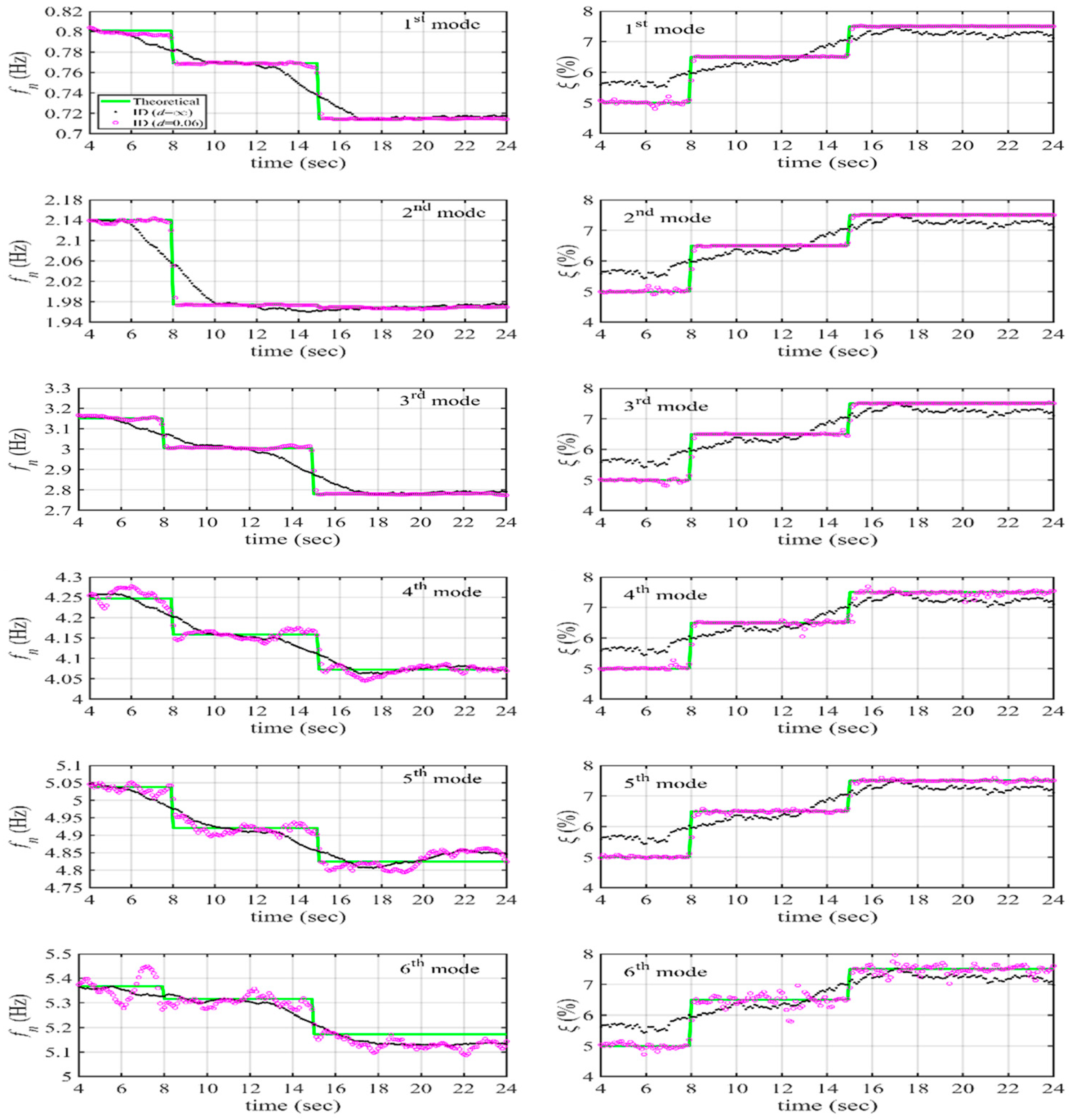
3.3. Sharply Varying System

The six-story shear building examined in this section is identical to the one discussed in the preceding section, with the exception of the parameters described as follows:

$$k_1=\{\begin{array}{cc}1800& 0\le t\le 8\\ 1800\left[1-0.2\left(t-8\right)/0.005\right]& 8<t<8.005\\ 1152& 8.005\le t\end{array},$$

$$k_3=\{\begin{array}{cc}600& 0\le t\le 15\\ 600\left[1-0.2\left(t-15\right)/0.005\right]& 15<t<15.005\\ 384& 15.005\le t\end{array},$$

$${\xi }_i=\{\begin{array}{cc}0.05& 0\le t\le 8\\ 0.05\left[1+0.3\left(t-8\right)/0.005\right]& 8<t<8.005\\ 0.065& 8.005\le t\le 15\\ 0.065\left[1+\frac{2}{13}\left(t-15\right)/0.005\right]& 15<t<15.005\\ 0.075& 15.005\le t\end{array} (\mathrm{for} i=1,2,\dots ,6).$$

The first mode scalogram of the sixth-floor responses (Figure 7c) indicates sharp changes in frequency.

Utilizing the same windows and weighting function outlined in Section 3.2, we processed the noisy base excitation and acceleration responses from the first and sixth floors within subspaces at level 6 of the SWPT. This methodology yielded time-varying identified frequencies and modal damping ratios for all six modes, as depicted in Figure 10. In employing the weighting function with ‘d’ set to 0.06, the identified results obtained using the weighting function with ‘d’ set to 0.06 s exhibited excellent agreement with the analytical values. The maximum differences of the first three modes in frequency were less than 4%, while the differences were less than 2% for the four and sixth modes. Regarding modal damping ratios, the maximum differences were less than 15% for the first sixth mode. These identified results markedly outperformed those obtained without the weighting function, especially in precisely capturing the abrupt changes in the frequency and damping ratio.

4. Applications to Real Measured Responses

Having demonstrated the effectiveness of the current approach in handling numerically simulated responses, we extend its application to process actual measured responses from a two-span cable-stayed bridge subjected to an earthquake. Additionally, we employed the approach in the analysis of nonlinear responses from a five-story steel frame under a shaking table test.

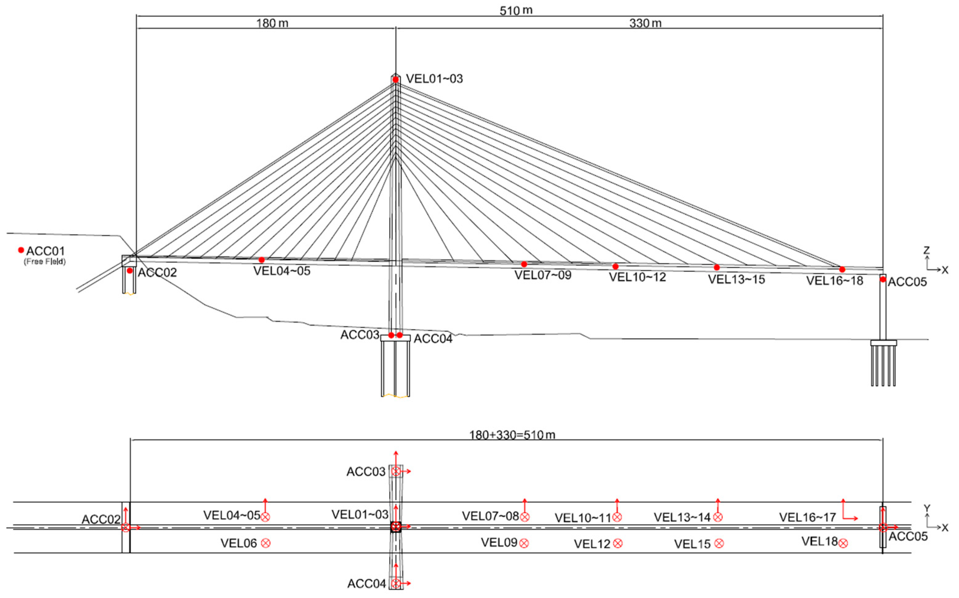
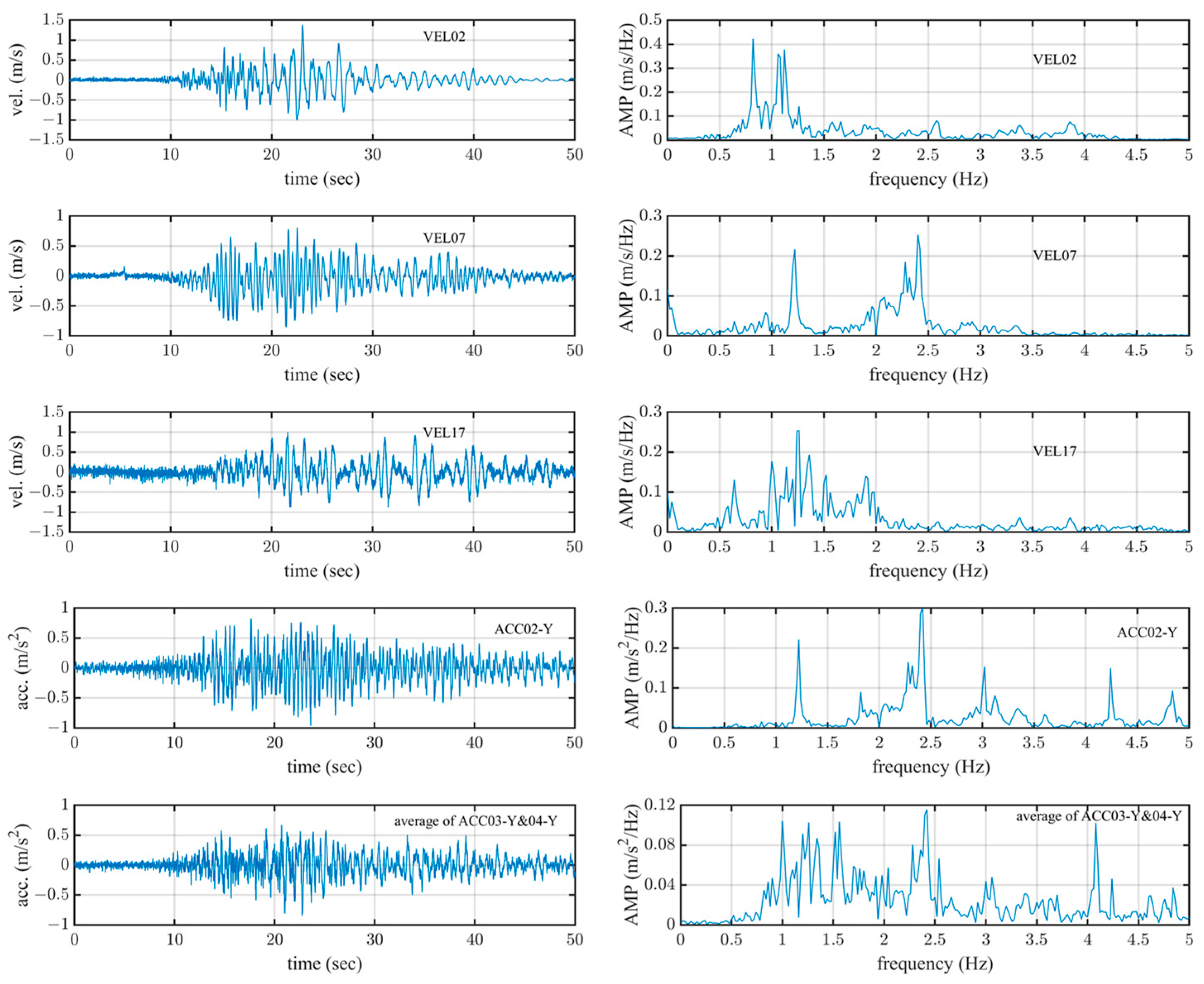
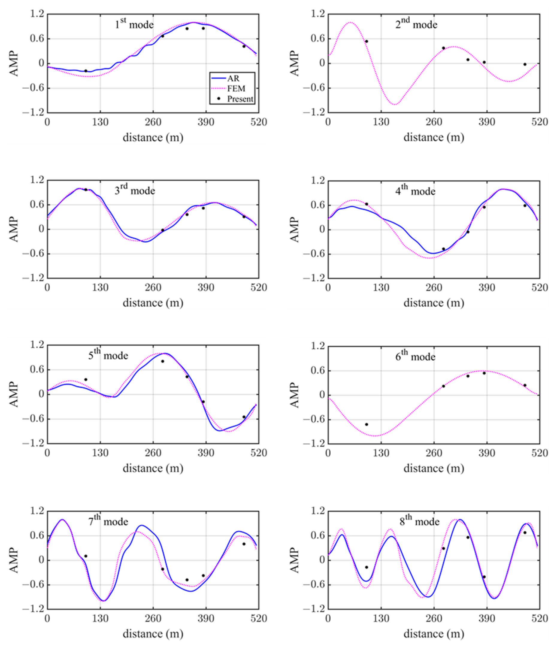
4.1. Application to a Two-Span Cable-Stayed Bridge

The considered two-span bridge, illustrated in Figure 11, is situated on Freeway 3 in Taiwan and features a 34.5 m wide deck. Comprising a 330 m long steel main span and a 180 m long prestressed concrete side span, the bridge is supported by a 183.5 m tall pylon with an inverted Y-shaped reinforced concrete structure and a diaphragm wall foundation. The pylon’s two legs are interconnected by a transverse beam. The bridge is supported by 60 steel cables in total, ensuring stability and structural integrity.

A comprehensive monitoring system was installed to measure the dynamic responses of the bridge in the face of wind and earthquake forces. A portion of this monitoring system is presented in Figure 11, with other sensors placed along the cables omitted from the illustration, as they were not utilized in this study. Three-axis accelerometers (ACC) and one-axis velocity meters (VEL) were strategically placed, including at locations such as the abutment (ACC 02), within the box girder of the deck (VELs 04–15), near the cable on the deck slab (VELs 16–18), atop a pylon (VELs 01–03), on the foundation (ACCs 03 and 04), and at pier P2 (ACC 05). The positions of these sensors are marked by red dots in Figure 11.

The proposed approach was employed to identify the modal parameters of the bridge in the transverse direction using earthquake measurements. Transverse acceleration measurements from ACCs 03 and 04 were averaged and treated as the transverse base excitations at P1. Additionally, the transverse acceleration measurements of ACCs 02 and 05 were considered base excitation inputs. Transverse velocity measurements of VELs 02, 04, 07, 10, and 17 were used as responses. Figure 12 illustrates the measurements from some of these sensors along with the corresponding Fourier spectra. The Fourier spectra of base excitations clearly indicate that the bridge was subjected to multiple base excitations.

Although not presented here, the first mode scalogram from the measurement of VEL 02 suggests that the bridge exhibited linear behavior during the considered earthquake. Data within the time interval of 20 to 30 s were processed using the proposed approach, identifying eight modes. The identified modal frequencies and damping ratios are provided in

Table 2. Identified modal parameters of the cable-stay bridge.

Mode		1	2	3	4	5	6	7	8
Present	ƒn (Hz)	0.64	1.19	1.71	2.21	2.53	2.83	3.14	3.82
	ξ	0.038	0.032	0.033	0.034	0.029	0.036	0.029	0.028
	MAC	0.98	0.97	0.99	0.99	0.97	0.99	0.97	0.98
Ambient vibrations [55]	ƒn (Hz)	0.65	/	1.64	2.19	2.57	/	3.17	3.89
	ξ	0.026	/	0.027	0.024	0.029	/	0.026	0.028
	MAC	0.97	/	0.98	0.97	0.97	/	0.96	0.98
FEM	ƒn (Hz)	0.65	1.17	1.68	2.15	2.49	2.81	3.15	3.95
	MAC	1	1	1	1	1	1	1	1

, while the identified modal shapes for the bridge deck are depicted in Figure 13. Table 2 and Figure 13 also include results obtained from a commercial finite element package based on design data and from an autoregressive (AR) time series model applied to the ambient vibration responses of the bridge [55]. The shown MAC values for the obtained modal shapes were computed with respect to those obtained from the finite element analysis. The present results align well with those from the finite element analysis and Su et al. [55]. Notably, the second and sixth modes identified from the present approach were not found by Su et al. [55] processing ambient vibration measurements along the bridge deck. This discrepancy is attributed to these two modes being dominated by the pylon, with the ratios of the identified modal component at the top of the pylon to the maximum modal component along the deck being approximately 41 and 6 for the second and sixth modes, respectively.

4.2. Application to a Five-Story Steel Frame

The investigated frame, illustrated in Figure 14, has dimensions of 3 m in length, 2 m in width, and a height of 13 m. Each floor was loaded with lead blocks to achieve an approximate mass of 3664 kg per floor. In subjecting the frame to a base excitation equivalent to 60% of the intensity of the Kobe earthquake, as shown in Figure 15, the acceleration responses of the first and fifth floors in the long-span direction (denoted as the x-direction in Figure 14) were recorded at a sampling rate of 250 Hz. These data served as input for identifying the modal parameters of the frame.

Huang et al. [19] observed clear permanent strains in the measured strains at a column of the first story, indicating the yielding of the steel columns under the considered base excitation. Although not presented here, the first mode scalogram from the measurement of the fifth floor illustrates the variation in the fundamental frequency over time, suggesting nonlinear behavior in the frame under the considered base excitations. It is worth noting that in a nonlinear system, the stiffness and damping matrices can be functions of displacement or velocity responses, which in turn depend on time. Consequently, the instantaneous modal parameters of the system exhibit time variation, and our proposed approach is capable of identifying these time-varying modal parameters, as demonstrated below.

Assuming rigid floors, which are commonly employed in building designs, the frame can be simplified into a five-degrees-of-freedom system in each of its long-span and short-span directions. Modal parameter identification involved windowed responses with a window length of 2 L, equal to 2 s. In Equation (25), the parameter ‘d’ in the weighting function was set to 0.06 s, and adjacent windows had an overlay of 1.9 s. The proposed approach yielded time-varying modal frequencies and modal damping ratios for five modes, as depicted in Figure 16. Figure 16 also includes results from Huang et al. [19], who utilized a time-varying autoregressive model with exogenous input (TVARX) with the continuous Cauchy wavelet transform to process responses from all five floors. The identified results from the present study exhibit favorable agreement with the published findings.

Figure 16 reveals significant variations in natural frequencies and modal damping ratios over time when 4.5 s < t < 7 s. Such variations indicate that the frame exhibited nonlinear behaviors under the considered base excitations within this time range. These nonlinear behaviors are indicative of earthquake-induced damage to the frame. Beyond this specific interval, the frame behaved linearly, and the variations in identified modal parameters with time are not as significant as the published ones.

5. Concluding Remarks

A novel approach that integrates the subspace method with the SWPT was developed for identifying the modal parameters in structures, encompassing both linear and nonlinear behaviors. The introduction of a Gaussian weighting function, coupled with a moving window technique, enhances the approach’s accuracy in identifying time-varying modal parameters. Leveraging the Meyer wavelet as a band-pass filter and its corresponding scale function as a low-pass filter constructs the basis functions for SWPT subspaces. The fine filtering properties inherent in the SWPT not only facilitate mode discrimination but also enable the identification of numerous modes from a limited number of measured degrees of freedom.

The validation of the proposed approach commenced with the processing of numerically simulated acceleration responses from six-story shear buildings, exhibiting constant, periodically time-varying, or sharply time-varying stiffness and modal damping ratios. The results underscore the effectiveness and robustness of the method in accurately determining time-varying modal parameters, even when base excitation and the responses of only two floors, with a 10% NSR, were utilized. Compared with true values, the identified frequencies and modal damping ratios for all six modes in the time-invariant shear building exhibited maximum differences of 0.9% and 5%, respectively. For the periodically time-varying shear building, the maximum differences in frequency were less than 1% for all six modes, with maximum modal damping ratio differences less than 15% for the first five modes and 20% for the sixth mode. In the case of the sharply time-varying shear building, the identified frequencies for the first four modes deviated by less than 1%, while the differences were less than 2% for the fifth and sixth modes. Correspondingly, the identified modal damping ratios differed from the true values by less than 15%.

In extending the application of the proposed approach, it was employed to process measured linear transverse velocity responses and support acceleration excitations from a two-span cable-stayed bridge during an earthquake, as well as nonlinear acceleration responses from the two floors of a five-story steel frame under a shaking table test. The identified modal parameters for the first eight transverse modes of the bridge demonstrated admirable agreement with those obtained from finite element analysis and ambient vibration measurements. Moreover, the identified time-varying modal parameters for the steel frame exhibited favorable agreement with published findings obtained using a time-varying autoregressive model with exogenous input with the continuous Cauchy wavelet transform. Significant changes in the natural frequencies and damping ratios indicated earthquake-induced damage to the frame. Overall, the proposed approach showcased its versatility and efficacy in accurately identifying modal parameters for structures undergoing both linear and nonlinear dynamic conditions.

References

1. Collura, D.; Nascimbene, R. Comparative assessment of variable loads and seismic actions on bridges: A case study in Italy using a multimodal approach. Appl. Sci. 2023, 13, 2771. [Google Scholar] [CrossRef]
2. Zhang, H.; Reuland, Y.; Shan, J.; Chatzi, E. Post-earthquake structural damage assessment and damage state evaluation for RC structures with experimental validation. Eng. Struct. 2024, 304, 117591. [Google Scholar] [CrossRef]
3. Farrar, C.R.; Doebling, S.W.; Nix, D.A. Vibration-based structural damage identification. Philos. Trans. R. Soc. A Math. Phys. Eng. Sci. 2001, 359, 131–150. [Google Scholar] [CrossRef]
4. Qarib, H.; Adeli, H. Recent advances in health monitoring of civil structures. Sci. Iran. Trans. A Civ. Eng. 2014, 21, 1733–1742. [Google Scholar]
5. Sony, S.; Laventure, S.; Sadhu, A. A literature review of next-generation smart sensing technology in structural health monitoring. Struct. Control. Health Monit. 2019, 26, e2321. [Google Scholar] [CrossRef]
6. Sirca, G.F.; Adeli, H. System identification in structural engineering. Sci. Iran. Trans. A Civ. Eng. 2012, 19, 1355–1364. [Google Scholar] [CrossRef]
7. Perez-Ramirez, C.A.; Amezquita-Sanchez, J.P.; Adeli, H.; Valtierra-Rodriguez, M.; Romero-Troncoso, R.J.; Dominguez-Gonzalez, A.; Osornio-Rios, R.A. Time-frequency techniques for modal parameters identification of civil structures from acquired dynamic signals. J. Vibroenginerring 2016, 18, 3164–3185. [Google Scholar] [CrossRef]
8. Shokravi, H.; Shokravi, H.; Bakhary, N.; Rahimian Koloor, S.S.; Petru, M. Health monitoring of civil infrastructures by subspace system identification method: An overview. Appl. Sci. 2020, 10, 2786. [Google Scholar] [CrossRef]
9. Safak, E.; Celebi, M. Seismic response of Transamerica building, II: System identification. J. Struct. Eng. ASCE 1991, 117, 2405–2425. [Google Scholar] [CrossRef]
10. Loh, C.H.; Lin, H.M. Application of off-line and on-line identification techniques to building seismic response data. Earthq. Eng. Struct. Dyn. 1996, 25, 269–290. [Google Scholar] [CrossRef]
11. Huang, C.S.; Hung, S.L.; Lin, C.I.; Su, W.C. A wavelet-based approach to identifying structural modal parameters from seismic response and free vibration data. Comput. Aided Civil Infrastruct. Eng. 2005, 20, 408–423. [Google Scholar] [CrossRef]
12. Huang, C.S.; Su, W.C. Identification of modal parameters of a time invariant linear system by continuous wavelet transformation. Mech. Syst. Signal Process. 2007, 21, 1642–1664. [Google Scholar] [CrossRef]
13. Satio, T.; Yokota, H. Evaluation of dynamic characteristics of high-rise buildings using system identification. J. Wind Eng. Ind. Aerodyn. 1996, 59, 299–307. [Google Scholar] [CrossRef]
14. Moore, S.M.; Lai, J.C.S.; Shankar, K. ARMAX modal parameter identification in the presence of unmeasured excitation-I: Theoretical background. Mech. Syst. Signal Process. 2007, 21, 1601–1615. [Google Scholar] [CrossRef]
15. Moore, S.M.; Lai, J.C.S.; Shankar, K. ARMAX modal parameter identification in the presence of unmeasured excitation-II: Numerical and experimental verification. Mech. Syst. Signal Process. 2007, 21, 1616–1641. [Google Scholar] [CrossRef]
16. Dziedziech, K.; Czop, P.; Staszewski, W.J.; Uhl, T. Combined non-parametric and parametric approach for identification of time-variant systems. Mech. Syst. Signal Process. 2018, 103, 295–311. [Google Scholar] [CrossRef]
17. Niedźwiecki, M. Identification of Time-Varying Processes; John Wiley & Sons: New York, NY, USA, 2000. [Google Scholar]
18. Loh, C.H.; Lin, C.Y.; Huang, C.C. Time domain identification of frames under earthquake loadings. J. Eng. Mech-ASCE 2000, 126, 693–703. [Google Scholar] [CrossRef]
19. Huang, C.S.; Liu, C.Y.; Su, W.C. Application of Cauchy wavelet transformation to identify time-variant modal parameters of structures. Mech. Syst. Signal Process. 2016, 80, 302–323. [Google Scholar] [CrossRef]
20. Van Overschee, P.; De Moor, B. Subspace Identification of Linear Systems: Theory, Implementation, Applications; Kluwer Academic Publishers: Dordrecht, The Netherlands, 1996. [Google Scholar]
21. Shokravi, H.; Shokravi, H.; Bakhary, N.; Heidarrezaei, M.; Rahimian Koloor, S.S.; Petru, M. Application of the subspace-based methods in health monitoring of civil structures: A systematic review and meta-analysis. Appl. Sci. 2020, 10, 3607. [Google Scholar] [CrossRef]
22. Li, Z.; Fu, J.Y.; Liang, Q.S.; Mao, H.J.; He, Y.C. Modal identification of civil structures via covariance-driven stochastic subspace method. Math. Biosci. Eng. 2019, 16, 5709–5728. [Google Scholar] [CrossRef] [PubMed]
23. Wang, C.; Hu, M.H.; Jiang, M.H.; Zuo, Z.N.; Zhu, Y.F.; Zhu, Z.Q. A modal parameter identification method based on improves covariance-driven stochastic subspace identification. ASME J. Eng. Gas Turbines Power. 2020, 142, 061005. [Google Scholar] [CrossRef]
24. Cheynet, E.; Daniotti, N.; Jakobsen, J.B.; Snaebjörnsson, J. Improved long-span bridge modeling using data-driven identification of vehicle-induced vibrations. Struct. Control. Health Monit. 2020, 27, e2574. [Google Scholar] [CrossRef]
25. Niu, Y.B.; Ye, Y.; Zhao, W.J.; Shu, J.P. Dynamic monitoring and data analysis of a long-span arch bridge based on high-rate GNSS-RTK measurement combining CF-CEEMD method. J. Civ. Struct. Health Monit. 2020, 11, 35–48. [Google Scholar] [CrossRef]
26. Liu, Y.K.; Loh, C.S.; Ni, Y.Q. Stochastic subspace identification for output-only modal analysis: Application to super high-rise tower under abnormal loading condition. Earthq. Eng. Struct. Dyn. 2013, 42, 477–498. [Google Scholar] [CrossRef]
27. Pioldi, F.; Rizzi, E. Assessment of frequency versus time domain enhanced technique for response-only modal dynamic identification under seismic excitation. Bull. Earthq. Eng. 2018, 16, 1547–1570. [Google Scholar] [CrossRef]
28. Allemang, R.L.; Brown, D.L. A correlation coefficient for modal vector analysis. In Proceedings of the First International Modal Analysis Conference, Bethel, CT, USA, 6–9 April 1983; pp. 110–116. [Google Scholar]
29. Kim, J.; Lynch, J.P. Subspace system identification of support-excited structures—Part I: Theory and black-box system identification. Earthq. Eng. Struct. Dyn. 2012, 41, 2235–2251. [Google Scholar] [CrossRef]
30. Kim, J.; Lynch, J.P. Subspace system identification of support excited structures—Part II: Gray-box interpretations and damage detection. Earthq. Eng. Struct. Dyn. 2012, 41, 2253–2271. [Google Scholar] [CrossRef]
31. Mellinger, P.; Döhler, M.; Mevel, L. Variance estimation of modal parameters from output-only and input/output subspace-based system identification. J. Sound Vib. 2016, 379, 1–27. [Google Scholar] [CrossRef]
32. Moonen, M.; De Moor, B.; Vandenberghe, L.; Vandewalle, J. On and off-line identification of linear state space models. Int. J. Control 1989, 49, 219–232. [Google Scholar] [CrossRef]
33. Van Overschee, P.; De Moor, B. N4SID: Subspace algorithms for identification of combined deterministic-stochastic systems. Automatica 1994, 30, 75–93. [Google Scholar] [CrossRef]
34. Viberg, M.; Wahlbergs, B.; Otterstens, B. Analysis of state space system identification methods based on instrumental variables and subspace fitting. Auromatica 1997, 33, 1603–1616. [Google Scholar] [CrossRef]
35. Mastronardi, N.; Kressner, D.; Sima, V.; Van Dooren, P.; Van Huffel, S. A fast algorithm for subspace state-space system identification via exploitation of the displacement structure. J. Comput. Appl. Math. 2001, 132, 71–81. [Google Scholar] [CrossRef]
36. Yu, D.J.; Ren, W.X. EMD-based stochastic subspace identification of structures from operational vibration measurements. Eng. Struct. 2005, 27, 1741–1751. [Google Scholar] [CrossRef]
37. Altunisik, A.C.; Sunca, F.; Sevim, F. Modal parameter identification and seismic assessment of historical timber structures under near-fault and far-fault ground motions. Structures 2023, 49, 1624–1651. [Google Scholar] [CrossRef]
38. Gandino, E.; Garibaldi, L.; Marchesiello, S. Covariance-driven subspace identification: A complete input–output approach. J. Sound Vib. 2013, 332, 7000–7017. [Google Scholar] [CrossRef]
39. Verhaegen, M.; Hansson, A. N2SID: Nuclear norm subspace identification of innovation models. Automatica 2016, 72, 57–63. [Google Scholar] [CrossRef]
40. Juang, J.N. System realization using information matrix. J. Guid. Control Dyn. 1997, 20, 492–500. [Google Scholar] [CrossRef]
41. Siringoringo, D.M.; Fujino, Y. Influence of movable bearings performance on the dynamic characteristics of a cable-stayed bridge: Insights from seismic monitoring records. Bull. Earthq. Eng. 2022, 20, 4639–4671. [Google Scholar] [CrossRef]
42. Oku, H.; Kimura, H. A recursive 4SID from the input-output point of view. Asian J. Control 1999, 1, 258–269. [Google Scholar] [CrossRef]
43. Oku, H.; Kimura, H. Recursive 4SID algorithms using gradient type subspace tracking. Automatica 2002, 38, 1035–1043. [Google Scholar] [CrossRef]
44. Loh, C.H.; Chen, J.D. Tracking modal parameters from building seismic response data using recursive subspace identification algorithm. Earthq. Eng. Struct. Dyn. 2017, 46, 2163–2183. [Google Scholar] [CrossRef]
45. Huang, S.K.; Chen, J.D.; Loh, K.J.; Loh, C.H. Discussion of user-defined parameters for recursive subspace identification: Application to seismic response of building structures. Earthq. Eng. Struct. Dyn. 2020, 49, 1738–1757. [Google Scholar] [CrossRef]
46. Chopra, A.K. Dynamics of Structures. In Theory and Applications to Earthquake Engineering; Prentice Hall: Hoboken, NJ, USA, 2014. [Google Scholar]
47. Huang, C.S.; Lin, H.L. Modal identification of structures from ambient vibration, free vibration, and seismic response data via a subspace approach. Earthq. Eng. Struct. Dyn. 2001, 30, 1857–1878. [Google Scholar] [CrossRef]
48. Pesquet, J.C.; Krim, H.; Carfantan, H. Time-invariant orthonormal wavelet representations. IEEE Trans. Signal Process. 1996, 44, 1964–1970. [Google Scholar] [CrossRef]
49. Fowler, J. The redundant discrete wavelet transform and additive noise. IEEE Signal Process. Lett. 2005, 12, 629–632. [Google Scholar] [CrossRef]
50. Perez-Solano, J.J.; Felici-Castell, S.; Rodriguez-Hernandez, M.A. Narrowband interference suppression in frequency-hopping spread spectrum using undecimated wavelet packet transform. IEEE Trans. Veh. Technol. 2008, 57, 1620–1629. [Google Scholar] [CrossRef]
51. Mallat, S. A Wavelet Tour of Signal Processing, 2nd ed.; Academic: San Diego, CA, USA, 1999. [Google Scholar]
52. Viberg, M. Subspace-based methods for the identification of linear time-invariant systems. Automatica 1995, 31, 1835–1851. [Google Scholar] [CrossRef]
53. Verhaegen, M. Identification of the deterministic part of MIMO state space models given in innovations form from input-output data. Automatica 1994, 30, 61–74. [Google Scholar] [CrossRef]
54. Yang, Q.J.; Zhang, P.Q.; Liand, C.Q.; Wu, X.P. System theory approach to multi-input multi-output modal parameters identification method. Mech. Syst. Signal Process. 1994, 8, 159–174. [Google Scholar] [CrossRef]
55. Su, W.C.; Huang, C.S.; Chen, C.H.; Liu, C.Y.; Huang, H.C.; Le, Q.T. Identifying the modal parameters of a structure from ambient vibration data via the stationary wavelet packet. Comput. Aided Civil Infrastruct. Eng. 2014, 29, 738–757. [Google Scholar] [CrossRef]
Figure 1. Decomposition of subspace.
Applsci 14 02503 g001
Figure 2. (a) Plots for Meyer mother wavelet ϕ ( t ) and corresponding scale function ψ ( t ) ; (b) Fourier spectra of Meyer mother wavelet and scale function.
Applsci 14 02503 g002
Figure 3. Main preserved frequency ranges in different subspaces.
Applsci 14 02503 g003
Figure 4. A flowchart outlining the procedure of the approach for estimating modal parameters.
Applsci 14 02503 g004
Figure 5. Schematic of a six-story shear building.
Applsci 14 02503 g005
Figure 6. Time histories and Fourier spectra of the simulated acceleration responses of the six-story shear building.
Applsci 14 02503 g006
Figure 7. Scalograms of the responses of the six floors of shear buildings: (a) time-invariant system; (b) periodically varying system; (c) sharply varying system.
Applsci 14 02503 g007
Figure 8. The stabilization diagrams of the identified frequencies and damping ratio using different values of s: (a) using signals in U 6 ( 1 ) ; (b) using signals in U 6 ( 2 ) ; (c) using signals in U 6 ( 4 ) ; (d) using signals in U 6 ( 3 ) .
Applsci 14 02503 g008
Figure 9. Identified modal parameters for the periodically varying system.
Applsci 14 02503 g009
Figure 10. Identified modal parameters for the sharply varying system.
Applsci 14 02503 g010
Figure 11. Arrangement of monitoring instruments on the cable-stayed bridge.
Applsci 14 02503 g011
Figure 12. The time histories and corresponding Fourier spectra of transverse acceleration or velocity responses at different locations of the cable-stayed bridge under an earthquake.
Applsci 14 02503 g012
Figure 13. Mode shapes of the bridge in the transverse direction.
Applsci 14 02503 g013
Figure 14. Schematic of the five-story steel frame.
Applsci 14 02503 g014
Figure 15. The relative acceleration responses of the first and fifth floors of the steel frame under shaking table tests.
Applsci 14 02503 g015
Figure 16. Identified time-varying modal frequencies and damping ratios for the steel frame.
Applsci 14 02503 g016