Investigation of Modal Identification of Frame Structures Using Blind Source Separation Technique Based on Vibration Data

Abstract

This paper investigates system identification algorithms for modal identification of frame structures, such as a suspension bridge and an overhead transmission line-crossing frame, using ambient vibration measurements. The modal identification procedures include two novel blind source separation (BSS) algorithms, complexity pursuit method (CP) and generalized eigen decomposition method (GED), based on modern signal processing technology. Here, the frequency response function (FRF) method is introduced as an important reference to verify the effectiveness of the CP algorithm and GED algorithm. The effectiveness and accuracy of both types of algorithms are verified by numerical simulations and experiments on a suspension bridge. In addition, an engineering application of these two BSS methods is successfully implemented in an overhead transmission line-crossing frame. The results show that the two novel BSS learning rules (CP and GED) are capable of successfully identifying modal parameters of the civil structure under ambient excitation.

1. Introduction

Modal parameters (frequency, mode shape, and damping) reflect the dynamic characteristics of a structure, which are important references for structural damage identification and vibration control. Therefore, modal identification is an indispensable part in the fields of structural health monitoring and vibration attenuation.

For a civil structure, its performance under traffic, wind, and other loads depends on its stiffness, mass and damping characteristics, and their distribution. In this case, the modal model consisting of frequency, mode shape, and damping ratio is identified from vibration data. Traditionally, parameter estimation methods can be used to obtain experimental models based on measurable input and output data. However, it is difficult to measure the environmental excitation of civil structures, and the available information for system identification algorithms is the output. Ambient excitation is an important phenomenon in civil structures, which plays a vital role in their health monitoring. Nevertheless, measuring such excitation reliably poses practical challenges, making the output the only means to obtain relevant information for system identification algorithms. In circumstances where direct measurements of ambient excitation are not possible, output-only measurement, also referred to as ambient vibration testing, provides a practical alternative for stimulating the structure. This approach leverages the effects of various environmental factors, including wind, traffic, and environmental loads, to induce vibrations in the structure [1,2,3,4,5]. Despite its limitations, such as human structure interaction [6] and wind structure interaction [7], ambient vibration testing remains a valuable tool in assessing the dynamic behavior of civil structures, especially when direct excitation is unattainable.

With the development of modern signal processing technology, blind source separation [8,9,10] has rapidly developed as a powerful signal processing method. It is a combination of statistical signal processing, artificial neural networks, and information theory. Its main task is to separate and reconstruct the input signal or identify the system only by the output information of the system (the mixed signal), when the input information is unknown. The blind source separation technique [11] has been extensively utilized in various application domains, including communications [12], image processing [13], biomedical signal processing [14] and geospatial information processing [15]. In comparison to the traditional method which relies on the model assumption of the system, the blind source separation method has the advantages of simplicity, high computational efficiency, non-parameterization, no need to assume the behavior, and no prior information of the system. Consequently, BSS techniques were introduced for mechanical vibration signal processing [16], and a physical interpretation of the BSS problem for structural dynamics was later developed by expressing the system responses in terms of vibration modes and treating the modal responses as virtual sources to be extracted [17]. Under the assumption of independent source statistics, two common BSS algorithms, independent component analysis (ICA) [11] and second-order blind identification (SOBI) [18], were proposed for output-only identification of mechanical and structural systems, and their effectiveness was demonstrated through simulated data and experimental measurements [19,20]. However, these two BSS methods have some limitations. The ICA method is limited to undamped or lightly damped structures [21,22]; the SOBI method assumes a fixed source, which cannot meet the close modes and non-diagonalized damping cases in the practical application of civil infrastructure [23,24,25].

For handling the aforementioned issues in modal identification, a novel BSS method- complexity pursuit using temporal predictability proposed in [26] was first applied to structural identification [27]. Their numerical and experimental results demonstrated that the CP method achieved precise and reliable modal identification, and it could provide effective approximation to non-diagonalized high damping modes even in the case of close modes, as well as high damping modes excited by a nonstationary environment. In addition, generalized eigen decomposition is a simple BSS method based on second-order statistics [28,29,30]. Its basic idea is that the two correlation matrices of observed signals are composed of matrix bundles and decomposed into generalized eigenvector matrices; then, the transposition of generalized eigenvector matrices is exactly an estimation of the separation matrix. Compared with the ICA, SOBI, and CP algorithms, the GED algorithm does not need an iterative optimization calculation process, it can directly separate the source signal by solving a generalized eigenvalue problem. Thus, the GED algorithm has the benefits of rapid convergence, simplicity, and easy implementation. However, at present, these two algorithms have not been widely used; the CP algorithm has only been applied to assess the modal parameters of a basic steel frame structure, and the GED algorithm is still in the theoretical research stage. Therefore, considering the complexity of civil structures and their operation environment, utilizing the CP and GED algorithms as effective tools for modal identification of large civil structures remains a challenge.

This paper investigates the evaluation of system identification algorithms for modal parameter identification of civil structures (a suspension bridge and an overhead transmission line-crossing frame) based on ambient vibration measurement. Taking into account that the measured response is only an ambient response, which is also a random vibration signal, the signals separated by the CP and GED algorithms cannot be directly used to evaluate the damping ratios of the structures. For solving this problem, the random decrement technique (RDT) and Hilbert transform (HT) are introduced into the BSS algorithms; then, a joint system identification algorithm that relies upon output measurements is obtained.

This paper is structured as follows: Section 2 describes two novel BSS learning rules termed complexity pursuit and generalized eigen decomposition, intending to realize the modal parameter identification of structures; Section 3 demonstrates the ability of two proposed algorithms, CP and GED, for output-only modal identification, through using the simulation data of a suspension bridge mock-up; Section 4 focuses on verifying the effectiveness of the mentioned methods under a laboratory test environment; Section 5 presents the application of the two BSS methods in an overhead transmission line-crossing frame; lastly, Section 6 summarizes the findings and conclusions of the study.

2. Blind Source Separation Techniques

This section introduces two novel BSS learning rule termed complexity pursuit and generalized eigen decomposition. The procedure of these two BSS methods to realize the modal parameter identification of structures is discussed in detail.

2.1. BSS Model

The objective of BSS is to extract the source signal from the measured values x(t) of m sensors, which are assumed to be instantaneously mixed with each other. The mathematical expression of this problem is as follows:

$$\mathit{x}\left(t\right)=\mathit{A}\mathit{s}\left(t\right)={\displaystyle \sum _{i=1}^n{a}_i{s}_i\left(t\right)}.$$

(1)

The objective of BSS is to recover the mixing matrix A and the n sources s(t) = [s₁(t), …, s_n(t)]^T from the m measured mixtures x(t) = [x₁(t), …, x_m(t)]^T, a_i is the i-th column of A associated with s_i(t). BSS techniques, such as ICA, SOBI, CP, and GED, impose the condition m = n, where the number of mixtures is equal to the number of sources. This implies that the matrix A is square, and a reverse transformation is available.

$$\mathit{s}\left(t\right)={\mathit{A}}^{-1}\mathit{x}\left(t\right).$$

(2)

This significantly simplifies the BSS problem, because, once A is estimated, the source can be easily recovered by Equation (2). Additionally, the overdetermined BSS problem (m > n) can be resolved by transforming it into a square problem for dimensionality reduction through principal component analysis (PCA).

BSS algorithms assume that the source signals are statistically independent, thus allowing the blind source separation model to be estimated. To achieve this, the CP algorithm searches for the de-mixing matrix W such that the components y(t) = [y₁(t), …, y_n(t)]^T recovered by Equation (3) approximate the simplest sources s(t), and W = A⁻¹.

$$\mathit{y}\left(t\right)=\mathit{W}\mathit{x}\left(t\right)$$

(3)

Furthermore, the GED algorithm can be used to calculate A and s(t) through the generalized eigen decomposition technique.

2.2. Correspondence in Modal Coordinates

For a general motion system, its motion equation is

$$\mathit{M}\ddot{\mathit{x}}(t)+{\mathit{C}}_d\dot{\mathit{x}}(t)+\mathit{K}\mathit{x}(t)=\mathit{f}(t),$$

(4)

where the matrices K, C_d, and M represent stiffness, damping, and mass, respectively, and are symmetric and real-valued. The system response vector x(t) = [x₁(t), ..., x_m(t)]^T can take the form of acceleration, velocity, or displacement, while the external force vector f(t) is also considered.

The observed system response x(t) is employed as a mixed signal input to the blind source separation model with learning rules, under the assumption that it is composed of simple source signals independently driven by physical laws. This perspective is in accordance with the modal identification problem, which extends the coupled system response x(t) to a linear combination of decoupled modal responses, as illustrated in Equation (5) and Figure 1.

$$\mathit{x}\left(t\right)=\mathit{\Phi }\mathit{q}\left(t\right)={\displaystyle \sum _{i=1}^n{\phi }_i{q}_i\left(t\right)}.$$

(5)

The vibration mode matrix Φ contains the i-th column ${\phi }_i$, which corresponds to the i-th modal response q_i(t) in the modal response vector q(t) = [q₁(t), ..., q_n(t)]^T. The modal response vector q(t) can be recovered from x(t) through the following equation:

$$\mathit{q}\left(t\right)={\mathit{\Phi }}^{-1}\mathit{x}\left(t\right).$$

(6)

The blind source separation (BSS) learning rules are incorporated into the modal identification framework, allowing for the estimation of the system’s modal parameters. When the system response is input into the BSS model as a mixture, the relevant algorithms (e.g., CP and GED) can be used to blindly extract the modal matrix and time-domain modal response.

2.3. Complexity Pursuit Algorithm (CP)

The complexity of any mixture lies between the simplest and most complex sources of components [31]. Thus, the least complex signal extracted from a collection of mixed signals is assured to be the source signal. Concretely, CP can search for a de-mixing (row) vector w_i such that the component y_i(t) is recovered as

$${\mathit{y}}_i(t)={\mathit{w}}_i\mathit{x}\left(t\right),$$

(7)

which yields the least complexity, thus approaching the (simplest) source signal.

2.3.1. Complexity and Predictability

The complexity pursuit method seeks a weight vector, which provides a set of orthogonal projections of mixed signals to minimize the complexity of each extracted signal. A simple complexity measure can be formulated as predictability. If each value of a signal is easily predicted by the previous signal value, the signal has low complexity. On the contrary, if the successive value of a signal is independent and cannot be predicted, such a signal has high complexity.

The measure of temporal predictability ${\mathit{F} (\mathit{w}}_{\mathit{i}}, \mathit{x})$ is widely used to estimate the complexity of signals, specifically the signal y_i that is extracted using a given weight vector w_i, where ${\mathit{y}}_{\mathit{i}}{=\mathit{w}}_{\mathit{i}}^{\mathrm{T}}\mathit{x}$. In order to identify source signals that are more easily predictable, a comparison is made between the predictability of a specific source signal, q_i, and that of a mixture of signals. If a source signal is comparatively easy to predict, then the optimal value of the weight vector, w_i, that maximizes the predictability of the extracted signal, y_i, should correspond to the generation of that specific source signal (y_i = q_i). It is noteworthy that maximum predictability of the signal corresponds to minimum complexity and vice versa. Through the measure of temporal predictability, this study aims to identify the weight vectors which generate signals with relatively lower levels of complexity and to explore their potential applications in signal processing.

2.3.2. Measuring Complexity Using Signal Predictability

Simple exponential smoothing (SES) is an effective forecasting method for data points that do not exhibit any trend or seasonal behavior. It is based on the idea of using a weighted average of the past data points to make predictions about the future. The weights are exponentially decreasing, giving more importance to the most recent data points. SES is most effective as a forecasting method for quasi-periodic signals. Formally, the exponential smoothing equation is

$$\widehat{\mathit{y}}(t)=\alpha \mathit{y}(t-1)+\left(1-\alpha \right)\widehat{\mathit{y}}(t-1),\cdots 0\le \alpha \le 1,$$

(8)

where $\widehat{\mathit{y}}$(t) is the forecast for the next period, α is the smoothing constant, y(t − 1) stands for the observed value of the series in period t − 1, and $\widehat{\mathit{y}}$(t − 1) is the old forecast for period t − 1. This equation is based on the idea of weighting the most recent observation y(t − 1) with a weight α and the most recent forecast $\widehat{\mathit{y}}$(t − 1) with a weight of 1 − α. Equation (8) can be expanded as follows:

$$\widehat{\mathit{y}}(t)=\alpha \hspace{0.17em}\mathit{y}(t-1)+\alpha (1-\alpha )\mathit{y}\hspace{0.17em}(t-2)+\alpha {(1-\alpha )}^2\mathit{y}\hspace{0.17em}(t-3)+\cdots +\alpha {(1-\alpha )}^{t-1}\mathit{y}(1).$$

(9)

• Long-term predictor $\overline{\mathit{y}}$(t): α is in the range of 0 to 0.3, when α close to $\overline{\mathit{y}}$(t) ≈ 0;
• Short-term predictor $\widehat{\mathit{y}}$(t): α is in the range of 0.4 to 1.

In general, short-term forecast is more accurate than long-term forecast. Thus, the exponential smoothing method is more suitable for the recent prediction.

According to the SES method, a predictability measure F is defined according to the extracted signal ${\mathit{y}}_{\mathit{i}}{=\mathit{w}}_{\mathit{i}}^{\mathrm{T}}\mathit{x}$. For extracting the source signal y_i = q_i from a set of M signal mixtures x(t) = [x₁(t), ..., x_M(t)]^T, it is necessary to find the weight vector w_i that maximizes the predictability F of y_i, so as to minimize its complexity.

Stone [26] proposed a simple and robust measure of signal complexity, termed temporal predictability, which is defined as

$$F\left({\mathit{y}}_i\right)=\log \frac{V\left({\mathit{y}}_i\right)}{U\left({\mathit{y}}_i\right)}=\log \frac{{\displaystyle \sum _{t=1}^N{\left({\overline{y}}_i\left(t\right)-y_i\left(t\right)\right)}^2}}{{\displaystyle \sum _{t=1}^N{\left({\widehat{y}}_i\left(t\right)-y_i\left(t\right)\right)}^2}},$$

(10)

where ${\overline{y}}_i$(t) is the long-term predictor, and ${\widehat{\mathit{y}}}_i$(t) is the short-term predictor.

$$\begin{array}{l}{\overline{y}}_i\left(t\right)={\alpha }_L{y}_i\left(t-1\right)+\left(1-{\alpha }_L\right){\overline{y}}_i\left(t-1\right),\cdots 0\le {\alpha }_L\le 1\\ {\widehat{y}}_i\left(t\right)={\alpha }_S{y}_i\left(t-1\right)+\left(1-{\alpha }_S\right){\widehat{y}}_i\left(t-1\right),\cdots 0\le {\alpha }_S\le 1\end{array}$$

(11)

The parameter α can be defined using the half-life parameter h, where α_S and α_L correspond to the different ranges of α. The formula for α is

$$\alpha =2^{-1/h},$$

(12)

where h_S = 1, and h_L is an arbitrary value (e.g., 900,000) as long as h_L >> h_S [26].

2.3.3. Extracting a Single Signal

Equation (7) can be incorporated into Equation (10) as follows:

$$F\left({\mathit{y}}_i\right)=F({\mathit{w}}_i,\mathit{x})=\log \frac{V\left({\mathit{w}}_i,\mathit{x}\right)}{U\left({\mathit{w}}_i,\mathit{x}\right)}=\log \frac{{\mathit{w}}_i\overline{\mathit{R}}{\mathit{w}}_i^{\mathrm{T}}}{{\mathit{w}}_i\hat{\mathit{R}}{\mathit{w}}_i^{\mathrm{T}}},$$

(13)

where $\overline{\mathit{R}}$ and $\widehat{\mathit{R}}$ represent the long-term and short-term covariance between the mixtures, respectively. These matrices are square matrices with dimensions n × n.

Note that maximizing only V_i would result in a high variance signal with no constraints on its temporal structure. In contrast, minimizing only U would result in a DC signal. In both cases, trivial solutions would be obtained for w_i because V_i can be maximized by setting the norm of w_i to be large, and U can be minimized by setting w_i = 0. In contrast, the ratio V_i/U_i can be maximized only if two constraints are both satisfied: (1) y has a nonzero range (i.e., high variance); (2) the values in y change slowly over time. Note also that the value of F is independent of the norm of w_i, such that only changes in the direction of w_i affect the value of F⁴.

The elements of these matrices are defined as

$$\begin{array}{l}{\overline{r}}_{ij}={\displaystyle \sum _{t=1}^N\left(x_i\left(t\right)-{\overline{x}}_i\left(t\right)\right)\left(x_j\left(t\right)-{\overline{x}}_j\left(t\right)\right)}\\ {\widehat{r}}_{ij}={\displaystyle \sum _{t=1}^N\left(x_i\left(t\right)-{\widehat{x}}_i\left(t\right)\right)\left(x_j\left(t\right)-{\widehat{x}}_j\left(t\right)\right).}\end{array}$$

(14)

Calculation of the covariance matrices can be achieved through fast convolution, which is a computational technique that facilitates efficient processing of large datasets. Utilizing this technique, the CP learning rule can be applied to a group of mixtures x(t), enabling the search for the de-mixing vector w_i that maximizes the objective function F(·). This process can use the classic gradient ascent technique.

On the basis of Equation (13), the derivative of F with respect to w_i can be expressed as

$${\nabla }_{w_i}F=\frac{2{\mathit{w}}_i}{{\mathit{V}}_i}\overline{\mathit{R}}-\frac{2{\mathit{w}}_i}{{\mathit{U}}_i}\hat{\mathit{R}}.$$

(15)

The objective function F in Equation (15) can be expressed as a ratio of quadratic forms, which has a unique global maximum or minimum. To extract all latent sources simultaneously, Stone [26] proposed an effective algorithm, which is described below.

The gradient of F reaches zero in the solution, where

$${\nabla }_{w_i}F=\frac{2{\mathit{w}}_i}{{\mathit{V}}_i}\overline{\mathit{R}}-\frac{2{\mathit{w}}_i}{{\mathit{U}}_i}\hat{\mathit{R}}=0.$$

(16)

This can be rewritten as

$$\overline{\mathit{R}}{\mathit{w}}_i=\frac{{\mathit{V}}_i}{{\mathit{U}}_i}\hat{\mathit{R}}{\mathit{w}}_i.$$

(17)

The matrix W = (w₁, w₂, ..., w_M)^T can be obtained using a generalized eigenvalue routine, such as using the eigenvalue function W^T = eig ($\overline{\mathit{R}}$, $\widehat{\mathit{R}}$). As mentioned above, the eigenvector defines the maximum in F. Therefore, by leveraging temporal predictability, CP can accurately extract the time-domain modal responses q(t) that represent the component sources that are concealed within the system motion mixture x(t):

$$\mathit{q}\left(t\right)=\mathit{W}\mathit{x}\left(t\right).$$

(18)

On the basis of Equation (5), it is possible to obtain the mode shape $\Phi$:

$$\Phi ={\mathit{W}}^{-1}.$$

(19)

Figure 2 depicts the general flow of the mode extraction process using CP. Once the modal responses q(t) is extracted using CP, the frequency and damping ratio of each mode can be computed by applying Fourier transform and the logarithmic decrement technique, respectively.

2.4. Generalized Eigen Decomposition (GED)

According to Equations (1) and (3), the BSS method aims to extract independent sources from their observed mixtures, without prior knowledge of the mixing matrix A or the source signals s. In other words, given a set of mixed signals x, the BSS method seeks to find a separation matrix W such that the estimated sources $\widehat{\mathit{s}}$ = Wx are as independent as possible and approximate the true source s as closely as possible. The solution process generally includes two steps [9,32]. The initial step in the BSS method involves performing a whitening transformation on the observed mixtures. This transformation aims to linearly transform the measured data such that the correlation matrix of the output vector matches the identity matrix. At this stage, the dimensionality of the measured vector is reduced to match that of the source vector. Then, the next step in the BSS method is to estimate the separation matrix or the inverse of the mixing matrix A. Another method includes simultaneous diagonalization of matrix pencil (R_x1, R_x2), namely, generalized eigen decomposition (GED). The calculation method of a matrix includes considering two signals with distinct energy [33], calculating one matrix in the filtering version of a mixed signal [34], and calculating the delay correlation matrix [28,35,36].

According to $\widehat{\mathit{s}}$ = Wx, the goal of GED is to seek the separation matrix W which satisfies Equation (20).

$$\mathit{W}\mathit{A}=\mathit{P}.$$

(20)

If the P matrix is a diagonal matrix or a permutation matrix, then the estimated source signals $\widehat{\mathit{s}}$ are obtained by multiplying the separation matrix W with the observed mixtures x.

The generalized eigenvalue decomposition involves simultaneous diagonalization of two matrices, known as a matrix pencil. In the context of BSS, the matrix pencil is formed by the correlation matrices R_x1 and R_x2 of the observed mixtures and the estimated source signals, respectively. For a given set of observed mixtures, let X be an m × N matrix containing N samples of each of the m measured signals. The correlation matrices for X can be calculated as

$${\mathit{R}}_{x1}=\frac{1}{N}\mathit{X}{\mathit{X}}^{\mathrm{T}},{\mathit{R}}_{x2}=\frac{1}{N}\mathit{X}{\mathit{H}}^{\mathrm{T}}\mathit{H}{\mathit{X}}^{\mathrm{T}}.$$

(21)

In [9], the correlation matrix R_x2 is a time-delayed version of the estimated source signals, while R_x1 is described by Equation (21) as the correlation matrix of the observed mixtures. In [36], both matrices in the matrix pencil can be time-delayed. In particular, R_x2 for a delay d can be written as

$${\mathit{R}}_{x2}=\frac{1}{N-d}\mathit{X}{\mathit{H}}^{\mathrm{T}}{\mathit{X}}^{\mathrm{T}},$$

(22)

where R_x2 is obtained by applying a lower diagonal matrix H to the observed mixtures X. Specifically, for a delay of d samples, the matrix H has only one nonzero diagonal, which is the d-th diagonal below the main diagonal. If d = 0, the matrix H becomes the identity matrix and Equation (21) is obtained, which represents the correlation matrix of the observed mixtures without any time delay.

The sensor pencil is correlated with the pencil calculated from the source signal through the mixing matrix A as follows:

$${\mathit{R}}_{x1}=\mathit{A}{\mathit{R}}_{s1}{\mathit{A}}^{\mathrm{T}},{\mathit{R}}_{x2}=\mathit{A}{\mathit{R}}_{s2}{\mathit{A}}^{\mathrm{T}},$$

(23)

where (R_x1, R_x2) is the sensor pencil, (R_s1, R_s2) is the source matrix pencil, and A denotes the instantaneous mixing matrix. Using the matrix pencil (R_x1, R_x2), the generalized eigenvalue (GED) statement is

$${\mathit{R}}_{x2}\mathit{E}={\mathit{R}}_{x1}\mathit{E}\mathit{D},$$

(24)

where D is a diagonal m × m matrix with the eigenvalues of the matrix pencil (R_x1, R_x2) and E is a m × m eigenvector matrix. Considering that X is an instantaneous mixture of the source signals, i.e., X = As, the equation can be rewritten as

$$\mathit{A}{\mathit{R}}_{s2}{\mathit{A}}^{\mathrm{T}}\mathit{E}=\mathit{A}{\mathit{R}}_{s1}{\mathit{A}}^{\mathrm{T}}\mathit{E}\mathit{D}.$$

(25)

When the instantaneous mixing matrix A is invertible, we can multiply both sides of the GED statement by A⁻¹, set as follows:

$${\mathit{E}}_s={\mathit{A}}^{\mathrm{T}}\mathit{E},$$

(26)

which leads to the eigen decomposition of the source pencil:

$${\mathit{R}}_{s2}{\mathit{E}}_s={\mathit{R}}_{s1}{\mathit{E}}_s\mathit{D}.$$

(27)

Using above relationship, we can relate the columns of the eigenvector matrix E_s of the source matrix pencil (R_s1, R_s2) to the columns of the eigenvector matrix E of the observed mixtures.

When the instantaneous mixing matrix A is an m × n matrix with m > n, Equation (25) can be written using block matrix notation. Specifically, we can divide A into two blocks, A_H and A_L, where A_H is an n × n matrix and A_L is an (m − n) × n matrix. Similarly, we can divide E into two blocks, E_H and E_L, where E_H is an n × m matrix and E_L is an (m − n) × m matrix. Then, using matrix block operations, Equation (25) can be written as

$$\begin{array}{l}{\mathit{A}}_{\mathit{H}}{\mathit{R}}_{s2}\mathit{\Omega }={\mathit{A}}_H{\mathit{R}}_{s1}\mathit{\Omega }\mathit{D},\\ {\mathit{A}}_L{\mathit{R}}_{s2}\mathit{\Omega }={\mathit{A}}_L{\mathit{R}}_{s1}\mathit{\Omega }\mathit{D},\end{array}$$

(28)

where

$$\mathit{\Omega }={\mathit{A}}_H^{\mathrm{T}}{\mathit{E}}_H+{\mathit{A}}_L^{\mathrm{T}}{\mathit{E}}_L={\mathit{A}}^{\mathrm{T}}\mathit{E}.$$

(29)

If A_H is an invertible matrix, then the first equation in Equation (28) can be used to obtain the eigen decomposition of the source matrix pencil (R_s1, R_s2). When A_H is not invertible, then Ω has rank less than m, and we cannot obtain the complete eigen decomposition of the source matrix pencil using the GED method. In this case, Ω has (m − n) zero columns, corresponding to the null space of ${\mathit{A}}_H^{\mathrm{T}}$, and the eigenvalues in D that do not belong to the eigenvalue decomposition of (R_s1, R_s2) are not paired with eigenvectors of the pencil.

For BSS problems, the separation matrix W is obtained from the transpose of the eigenvector matrix E^T:

$$\widehat{\mathit{s}}=\mathit{W}\mathit{x}={\mathit{E}}^{\mathrm{T}}\mathit{x}.$$

(30)

If the source eigenvector matrix E_s is normalized to have unit length, then $\widehat{\mathit{s}}$ will be the estimated value of the source signal, but the magnitude and ordering are uncertain.

2.5. Extraction of Modal Parameters

In general, blind source separation methods such as CP and GED can separate the mixed sources up to a scaling and permutation ambiguity. This means that the estimated sources are only determined up to a scaling factor and a permutation of the sources, and the exact sequence and amplitude of the modal responses and mode shapes cannot be recovered directly from the separated sources. However, this ambiguity can be resolved by rearranging the modes on the basis of their frequency values [22]. Specifically, the recovered modal response and its associated mode shape vector with the smallest frequency can be recognized as the first mode, and so on, until all modes have been assigned to their correct order. This is based on the assumption that the modal responses and mode shapes are ordered in frequency, which is often the case in practice.

The modal assurance criterion (MAC) is a measure of the similarity between two mode shapes, which is commonly used to evaluate the correlation between the theoretical mode ${\mathit{\phi }}_i$ and the estimated mode ${\tilde{\mathit{\phi }}}_i$ obtained from BSS methods such as CP and GED. The MAC is defined as

$$MAC\left({\tilde{\mathit{\phi }}}_i,{\mathit{\phi }}_i\right)=\frac{{\left({\tilde{\mathit{\phi }}}_i^T\cdot {\mathit{\phi }}_i\right)}^2}{\left({\tilde{\mathit{\phi }}}_i^T\cdot {\tilde{\mathit{\phi }}}_i\right)\left({\mathit{\phi }}_i^T\cdot {\mathit{\phi }}_i\right)}.$$

(31)

The MAC ranges from 0 to 1, where a value of 1 indicates perfect correlation between the two mode shapes, and a value of 0 indicates no correlation. This study takes MAC values over 0.8 as a threshold criterion for identified mode shapes. In addition, it takes the error below 0.1 and 0.2 as the threshold criterion for identified frequencies and damping ratios, respectively. The natural frequency and damping can be obtained by measuring the time lapse and the logarithmic decrements between consecutive peaks of the trace of free-decay time history. Furthermore, accurately estimating the damping ratio in random vibration often requires additional preprocessing techniques. On the basis of RDT processing, the random response signal of a linear system is expected to exhibit similar characteristics to those observed in a free vibration response. In practical response histories, however, the peaks may not be captured exactly. For example, a peak may appear higher than its preceding peak because of nonlinearity, sampling, noise, and various other conditions, resulting in erroneous negative damping. The method presented in this study is based on the Hilbert transform. This method is more robust and considerably easier to apply than conventional methods.

With the Hilbert transform H[•], the analytic signal is defined as

$$z_i\left(t\right)={\widehat{q}}_i\left(t\right)+j\mathrm{H}[{\widehat{q}}_i\left(t\right)]=A_i(t)e^{-j{\theta }_i(t)},$$

(32)

where $\widehat{\mathit{q}}$(t) is the ith modal response q_i(t) processed by RDT method.

The instantaneous amplitude is defined as

$$A_i(t)=\sqrt{{\widehat{q}}_i^2\left(t\right)+{\mathrm{H}}^2[{\widehat{q}}_i\left(t\right)]}.$$

(33)

The phase function is defined as

$${\theta }_i(t)=\arctan \left(\frac{\mathrm{H}[{\widehat{q}}_i\left(t\right)]}{{\widehat{q}}_i\left(t\right)}\right).$$

(34)

The instantaneous frequency is simply expressed as

$${\omega }_i(t)=\frac{\mathrm{d}{\theta }_i(t)}{\mathrm{d}t}.$$

(35)

The magnitude and phase in the above equation can be further expressed as

$$A_i(t)=A_i{e}^{-{\xi }_i{\omega }_{i}t},{\theta }_i(t)={\omega }_{di}t+{\theta }_i.$$

(36)

According to Equation (36), the modal parameter identification equation can be obtained as

$$\ln A_i(t)=-{\xi }_i{\omega }_{i}t+\ln A_i,$$

(37)

$${\omega }_i(t)=\frac{\mathrm{d}{\theta }_i(t)}{\mathrm{d}t}={\omega }_{di}.$$

(38)

Thus, the damped angular frequencies ω_di and ξ_i ω_i can be obtained directly from the slopes of two straight lines of Equations (37) and (38). On the basis of Equation (39), t-he ith natural frequency ω_i and the damping ratio ξ_i can be obtained.

$${\omega }_{di}={\omega }_i\sqrt{1-{\xi }_i{}^2}.$$

(39)

The output-only BSS modal identification algorithms (CP and GED) presented in this study are capable of performing blind modal identification, as they can extract modal information directly from the measured structural responses. Their implementations are summarized in the flowchart in Figure 3.

3. Numerical Simulation

The objective of this section is to assess the effectiveness of CP and GED for output-only modal identification, and to compare the relative strengths and weaknesses of these two BSS methods. The dynamic responses of the suspension bridge mock-up were generated through a series of numerical simulations. Utilizing the aforementioned algorithms, both CP and GED were employed to extract the modal parameters of the suspension bridge under white-noise excitation.

3.1. Suspension Bridge System

To evaluate the effectiveness of modal identification methods, a low-damped suspension bridge model (Figure 4) was constructed and tested both numerically and experimentally. The validation of the numerical model was verified by a vibration test in a laboratory mock-up. The numerical and experimental modal parameters of the bridge mock-up are given in

Table 1. Numerical and the experimental natural frequencies and mode shapes of the mock-up.

Mode	Numerical [Hz]	Experimental [Hz]	Numerical Mode Shape 3	Experimental Mode Shape 4
1st B 1	4.7	5.1
2nd B	6.5	6
1st T 2	9.8	10.1
3rd B	12.3	11.8
2nd T	12.1	13.2
4th B	17.6	19.1

¹ B, bending mode; ² T, torsional mode; ³ The blue graphic represents the original form of the bridge deck, the green graphics represent the numerical mode shape the bridge deck; ⁴ The red graphics represent the experimental mode shape the bridge deck.

, as described in previous studies [37,38,39].

To investigate the effectiveness of CP and GED in handling random vibration, stationary Gaussian white noise (GWN) was employed to excite the system. The bridge deck was excited using a point force, as illustrated in Figure 4. Vertical acceleration of the deck was measured at 20 locations, situated in close proximity to the hangers. The hangers were numbered from 1 to 10 on one side, commencing from the right, and from 11 to 20 on the opposing side. To implement BSS methods for modal identification, the ambient vibration of the structure is required to be measured for a duration of at least 1000–2000 periods of the lowest natural frequency:

$$T_{\min }=\frac{1000\to 2000}{f_{\min }}\sec ,$$

(40)

where the lowest natural frequency in Hz, denoted as f_min, was determined to be approximately 5 Hz according to the initial FRF analysis. Accordingly, the recording time of 200 s was selected for the ambient vibration measurement. To simulate the actual test environment and investigate the robustness of the methods, zero-mean Gaussian white noise was introduced to the accelerometer outputs, with a standard deviation ranging from 1% to 5% of the signal level.

3.2. Simulation Results and Discussion

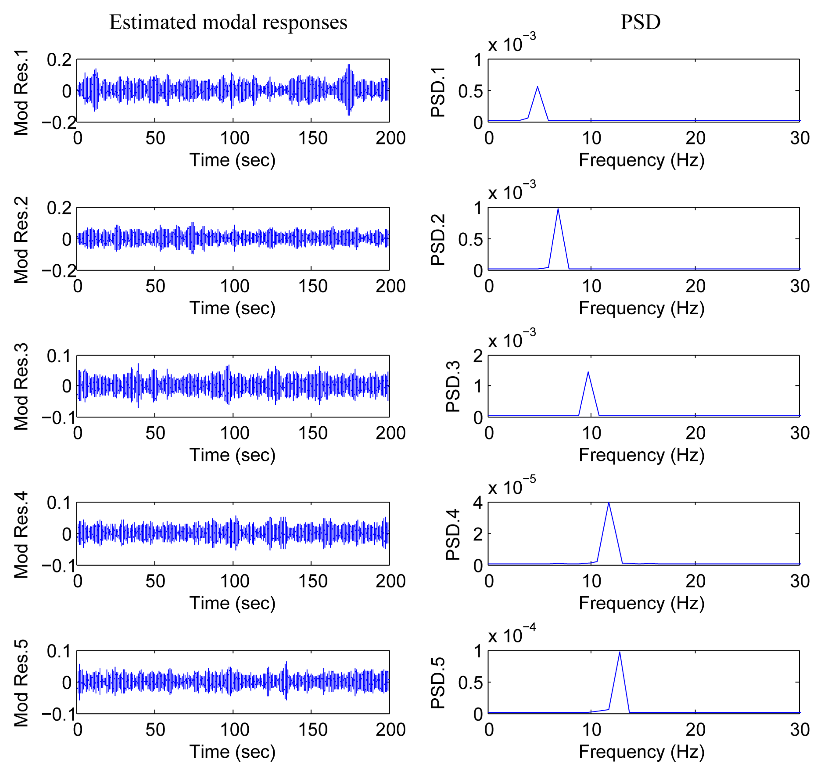
3.2.1. Results Analysis of Complexity Pursuit

Figure 5 illustrates the measured structure responses, while Figure 6 displays the reconstructed modal responses, indicating that the coupled random structure responses were effectively separated into distinct single-component modal responses. For conciseness, only the first five modes are given in Figure 6.

Table 2. Identification results by complexity pursuit in random vibration.

Mode	Theoretical Value		Identified (Without Noise)			Identified (1–5% RMS Noise)
	f (Hz)	ξ	f (Hz)	ξ	MAC	f (Hz)	ξ	MAC
1 (1st B)	4.69	0.01	4.67	0.009	1	4.66	0.012	1
2 (2nd B)	6.51	0.01	6.51	0.011	1	6.54	0.012	1
3 (1st T)	9.82	0.01	9.84	0.011	1	9.76	0.008	0.92
4 (2nd T)	12.07	0.01	12.04	0.008	0.74	12.11	0.006	0.69
5 (3rd B)	12.31	0.01	12.32	0.009	0.99	12.34	0.009	0.94
6	14.47	0.01	14.46	0.009	0.96	14.56	0.009	0.90
7 (4th B)	17.60	0.01	17.64	0.009	0.99	17.57	0.012	0.90
8	19.07	0.01	19.07	0.009	1	18.90	0.008	0.92
9	23.36	0.01	23.35	0.008	0.99	23.34	0.007	0.96

presents a comparison between the identified results obtained via the CP method and the theoretical results. If the noise effect is disregarded, the identified values of frequency (f), damping ratio (ξ), and mode shapes exhibited excellent agreement with the theoretical results, except for the mode shape of mode 4. As depicted in Figure 5, the fourth and fifth modes were closely spaced and challenging to differentiate on the basis of the PSD of the structural response. However, the CP method successfully separated these modes (as shown in Figure 6). Despite this, the CP method was unable to precisely determine the mode shape of these close modes. The sixth mode, eighth mode, and ninth mode were mixed modes, which could be accurately separated using the CP method.

As depicted in Figure 7, the identified frequencies and damping ratios remained consistent despite variations in the length of the time histories used to analyze the structure responses. The MAC values obtained from analyzing the structure responses with different sample lengths revealed high consistency, with all values above 0.90 (except mode 4). These results suggest that the accuracy of the CP method was not significantly affected by variations in sample length, indicating the method’s robustness.

It is worth mentioning that the identification ability of CP method hardly declined with 1–5% RMS noise added to the output data. As shown in Table 2, except for the damping ratio and mode shape of mode 4, other modal parameters were completely identified. The findings indicate that the CP method is highly robust to the effects of measured noise, as it was able to accurately recover the modal responses of the structure despite the presence of noise.

3.2.2. Results Analysis of Generalized Eigen Decomposition

Table 3. Identification results by generalized eigen decomposition in random vibration.

Mode	Theoretical Value		Identified (Without Noise)			Identified (1–5% RMS Noise)
	f (Hz)	ξ	f (Hz)	ξ	f (Hz)	ξ	f (Hz)	MAC
1 (1st B)	4.69	0.01	4.67	0.011	1	4.71	0.009	1
2 (2nd B)	6.51	0.01	6.51	0.01	1	6.55	0.011	1
3 (1st T)	9.82	0.01	9.82	0.009	1	9.83	0.008	0.95
4 (2nd T)	12.07	0.01	12.08	0.009	1	12.03	0.012	0.98
5 (3rd B)	12.31	0.01	12.34	0.011	0.97	12.37	0.006	1
6	14.47	0.01	14.51	0.012	0.93	--	--	--
7 (4th B)	17.60	0.01	17.60	0.008	1	17.63	0.008	0.98
8	19.07	0.01	19.05	0.01	1	--	--	--
9	23.36	0.01	23.36	0.01	1	--	--	--

shows a comparison between the identified results obtained using the GED method and the theoretical results. The comparison indicates that, without considering the impact of noise, the identified frequency, damping ratio, and mode shape closely matched the theoretical results, demonstrating excellent agreement between the two sets of data. Figure 8 presents the recovered modal responses in random vibration along with their corresponding power spectral density (PSD). It is important to note that the sequence of the recovered modal responses was not rearranged in order to display the original results obtained using the GED method. For example, the use of the term “modal response 1” in Figure 8 simply refers to the first response recovered by the GED method, and it does not necessarily correspond to mode 1 of the structure. This is a minor issue that can be easily resolved by rearranging the sequence of the recovered modal responses, as demonstrated in Figure 6 and explained in Section 2.5. It can be observed that the multicomponent structure responses were completely separated into monotone modal responses.

In addition, as presented in Figure 9, the identified frequencies and damping ratios were almost identical with different sample (window) lengths of the time histories of the structure responses. The MAC values of the identification remained very high with different sample (window) lengths of the time histories of the structure responses; all were above 0.90. The results indicate that the accuracy of the GED method is insensitive to the sample length.

Compared with the CP method, it is clear to see that the performance of this method was better, especially in the identification accuracy of the close space modes. When the 1–5% RMS noise was added to the structure responses, the procedures of the GED method were performed on the noise-contaminated system responses, and the identification results are given in Table 3. It can be seen that the identification results were seriously affected by the noisy data (failing to identify the mixed mode 6, 8 and 9); that is, the GED method was not robust once the measured noise was added.

4. Experimental Verification

4.1. Experimental Setup

The laboratory mock-up of the suspension bridge (in Figure 10) was used to verify the capability of the modal identification methods [37]. A voice coil vibrator was used to excite the structure (band-limited white noise). Prior to vibration measurements, the data acquisition system was established, which involved four single-axial accelerometers, positioned to measure vertical accelerations. The position of the accelerometers is illustrated in Figure 11a. The output data were obtained by repeated measurements, which covered all positions on the deck (Figure 11b). The sample setting was the same as Section 3.1. The modal parameters of the bridge were estimated by CP and GED.

4.2. Experimental Results and Discussion

Because of uncertainty, the identification of modal parameters for a real structure is more challenging than a numerical model. To verify the performance of above identification methods, the modal parameters generated by the classical input–output modal analysis algorithm (frequency response function method, FRF) are introduced as a reference. Through the peak-picking technology (PP), six modes could be accurately obtained within the range of 0–30 Hz. As usual, the damping ratios were more uncertain. Thus, both the FRF and the BSS methods could only get an estimation of the damping ratio. The identification accuracy of damping ratio can be referred to the simulation results in Section 3.2.

The modal parameters were identified using the methodology described in this study.

Table 4. Identification results by BSS methods in experimental test.

Mode	Input-Output (FRF)	Identified by CP			Identified by GED
	f (Hz)	f (Hz)/Error	ξ(%)	MAC	f (Hz)/Error	ξ(%)	MAC
1 (1st B)	5.12	5.13/0.20%	0.28	0.96	5.14/0.39%	0.29	0.96
2 (2nd B)	5.78	5.82/0.69%	1.48	0.86	5.80/0.35%	1.43	0.87
3 (1st T)	10.14	10.12/0.20%	0.60	0.82	10.15/0.10%	0.59	0.99
4 (3rd B)	11.76	--	--	--	11.62/1.19%	0.36	0.81
5 (2nd T)	13.20	13.18/0.15%	0.25	0.96	13.20/0%	0.19	0.98
6 (4nd B)	19.06	19.07/0.05%	0.21	0.96	19.06/0%	0.21	0.96
CPU Time		5.47 s			2.6 s

shows the identified modes for the mock-up using the CP and GED methods. It also shows the correlation of the output-only identification results with the input–output identification results. It is clear that the maximum identified frequency error between the BSS methods and FRF method was less than 1.5%; the mode shape correlation using the modal assurance criterion (between the identified modal vector and theoretical modal vector) was high, close to unity for most of the modes. In addition, the CPU time for CP and GED was only dependent on the length of the response signal; the computation time of GED was shorter than that of the CP method, taking only 2.6 s.

In Table 4, under the laboratory environment, the CP method missed mode 4, and the performance of GED was better than CP, but the identification accuracy of mode 4 decreased significantly. Here, the most reasonable explanation for this case is that mode 4 was not well excited (mode 4 corresponds to mode 3rd B in Table 1, the actuator close to the fixed node of mode 4). Overall, the identified natural frequencies from the GED method were in excellent agreement with the reference (FRF method), and the mode shapes were within reasonable agreement with the theoretical mode shapes. Figure 12 illustrates several representative modes identified using GED.

5. Application of BSS Methods in Overhead Transmission Line-Crossing Frame

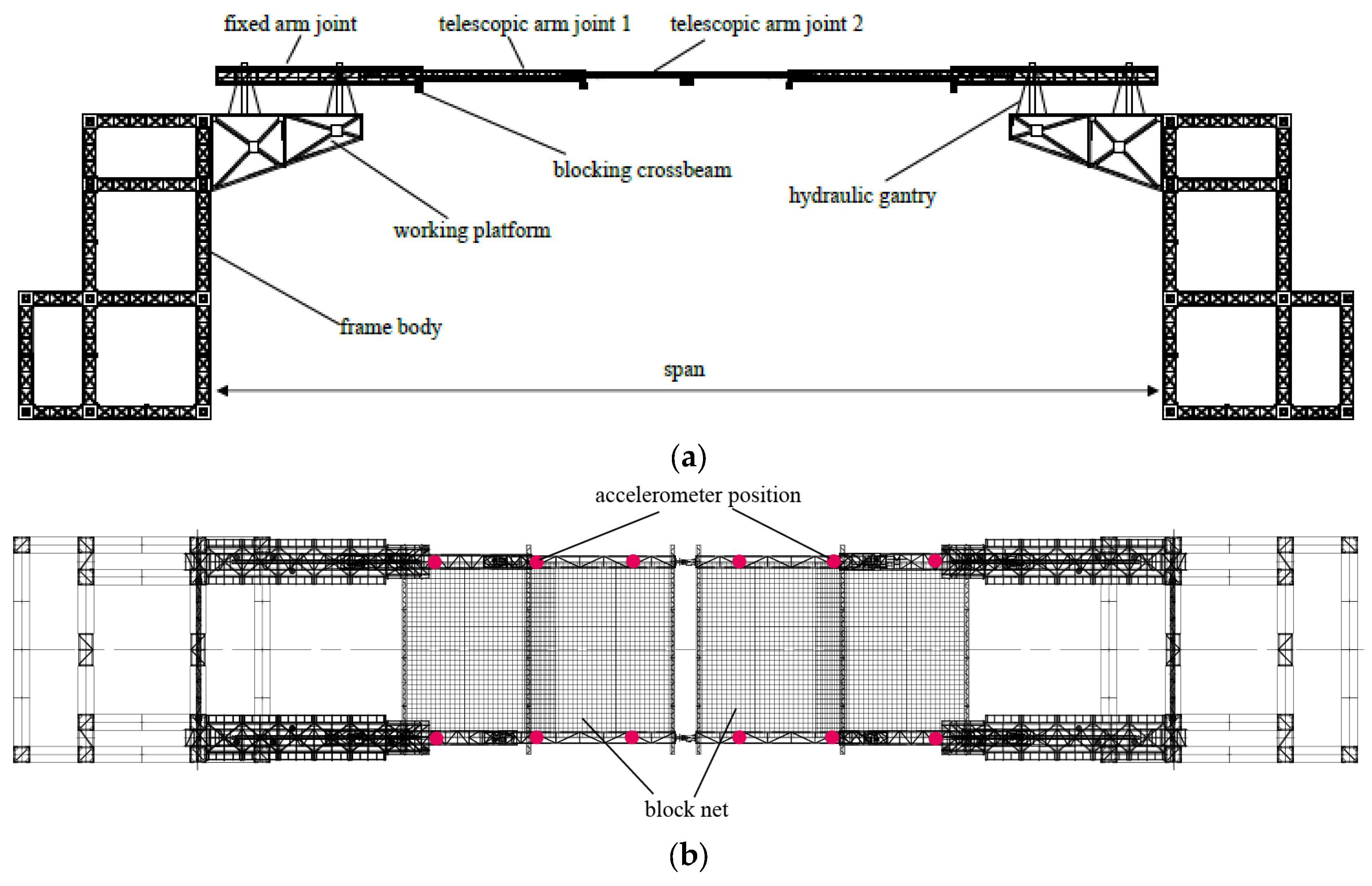
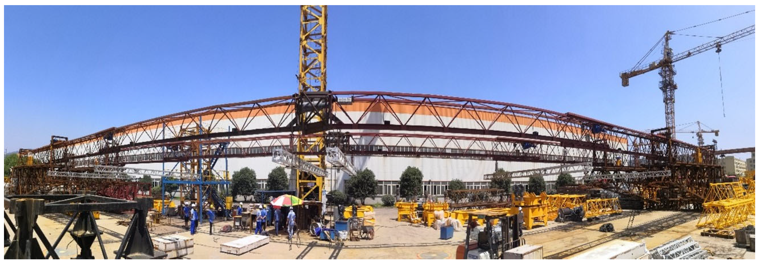
5.1. Overhead Transmission Line-Crossing Frame System

The crossing frame is an important equipment to ensure the safe construction of the transmission line, and the modal parameters are the key parameters for monitoring the structural health of the crossing frame. As a large civil structure, it is practically difficult to measure ambient excitation, and the output is the only information that can be used to modal identification. Hence, we attempted to use the CP and GED method to obtain the modal parameters of the crossing frame.

The crossing frame is mainly composed of a frame body, telescopic arm joint, working platform, hydraulic gantry, blocking crossbeam, transmission mechanism, power mechanism, docking mechanism, console, etc. A three-dimensional diagram is shown in Figure 13. The crossing frame met the requirements such as a maximum span of 60 m, a maximum span height of 30 m, a beam with a single side bearing of 20 kN, and an assembly time of less than 20 min.

The data acquisition system was established, which involved 12 three-axial JM3874 accelerometers (Figure 14), positioned to measure vertical accelerations. The position of the accelerometers is illustrated in Figure 13b. The output data were obtained by simultaneous measurements, which covered all positions on the arm joint (Figure 15). The sampling frequency was 64 Hz, and the sampling time was 15 min. The modal parameters of the crossing frame were estimated using CP and GED.

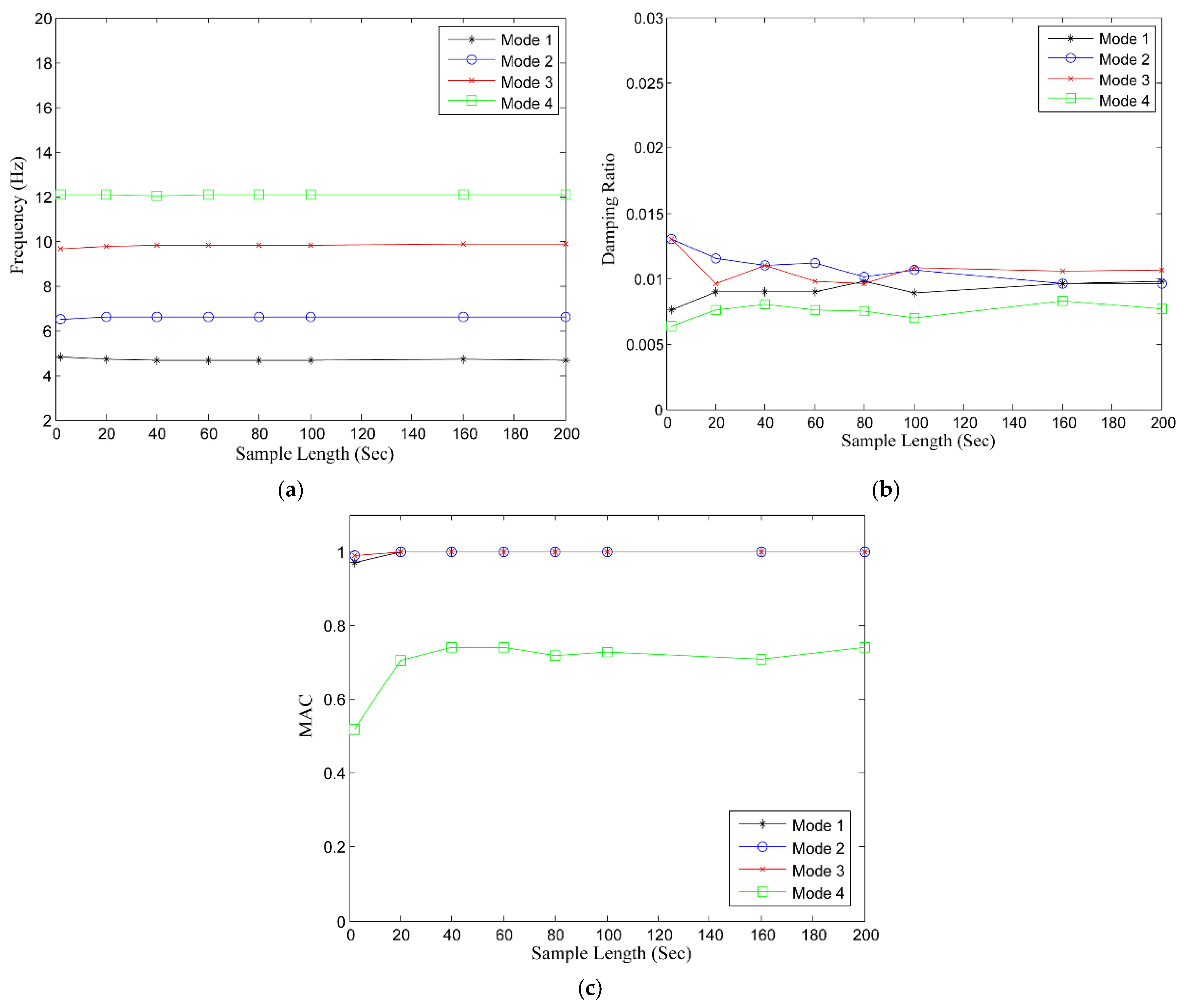
5.2. Result Analysis

Similarly, the FRF method was introduced as a reference. By manual selection of the eigenfrequencies (red lines), the spurious modes could be removed as shown in Figure 16. Five modes were accurately obtained using the FRF method; the modal parameters are shown in

Table 5. Modal parameters of the crossing frame (by FRF method).

Mode	f (Hz)	ξ (%)	Mode Shape 1
1st B	1.00	2.08
1st T	1.22	3.19
2nd B	1.59	1.04
2nd T	2.25	1.22
3rd B	4.44	0.59

¹ The colours represent the amplitude, the darker the colour the greater the amplitude.

.

The results identified using the CP and GED method are presented in

Table 6. Identification results of the crossing frame by CP and GED.

Mode	Input-Output (FRF)		Identified by CP			Identified by GED
	f (Hz)	ξ (%)	f (Hz)/Error	ξ (%)/Error	MAC	f (Hz)/Error	ξ (%)/Error	MAC
1 (1st B)	1.00	2.08	1.01/1.0%	1.98/4.8%	0.99	1.00/0%	2.16/3.8%	0.99
2 (1st T)	1.22	3.19	1.25/2.5%	3.05/4.4%	0.84	1.21/0.8%	3.21/0.6%	0.89
3 (2nd B)	1.59	1.04	1.52/4.4%	1.18/13.5%	0.92	1.60/0.6%	1.10/5.8%	0.98
4 (2nd T)	2.25	1.22	2.26/0.4%	1.25/2.5%	0.96	2.28/1.3%	1.31/7.4%	0.99
5 (3rd B)	4.44	0.59	4.47/0.7%	0.68/15.3%	0.89	4.43/0.2%	0.55/6.8%	0.91
CPU Time			7.52 s			4.65 s

. Compared with Table 5, it is clear that the maximum identified frequency difference between the BSS methods and the FRF method was less than 4.4%; the identified damping ratio was close to that obtained by the FRF method (maximum error 15.3%), with a high identified mode shape correlation using the modal assurance criterion (between the BSS methods and FRF method), being close to unity for most of the modes.

The test results indicate that the CP and GED method could identify the first five modes under the ambient excitation, which further verifies the effectiveness of the identification algorithm in civil structures.

6. Conclusions

This study presented a schematic data analysis and evaluation of modal identification procedures to obtain dynamic characteristics of civil structures (a suspension bridge and an overhead transmission line-crossing frame) using the ambient response. The band-limited white noise signal was used to simulate the ambient excitation source. The modal identification procedures included two types of output-only modal identification algorithms: the novel BSS learning rules (CP and GED) based on modern signal processing technology. The effectiveness and accuracy of both types of algorithms were investigated by numerical simulations and experiments in a suspension bridge. In addition, an engineering application of BSS methods was implemented in an overhead transmission line-crossing frame. On the basis of the presented results and interpretations, the main findings can be summarized as follows:

• This study explored the feasibility of the novel BSS learning rules CP and GED in modal identification of a suspension bridge. Comparison of these two methods showed that the GED method was accurate; however, as the noise increased, the accuracy declined severely. Under a laboratory environment, GED is more applicable because this method has higher computing efficiency and accuracy than CP. However, the CP method has efficient mixed modal identification capabilities. The disadvantage of the BSS method is that the order of identifiable modes is limited by the number of sensors and cannot identify the mode which is not always well excited by ambient sources.
• The CP and GED methods are capable of successfully identifying modal parameters of the crossing frame under ambient excitation, which further verifies the effectiveness of the identification algorithm in civil structures.

References

1. Siringoringo, D.M.; Fujino, Y. System identification of suspension bridge from ambient vibration response. Eng. Struct. 2008, 30, 462–477. [Google Scholar] [CrossRef]
2. Peeters, B.; Ventura, C.E. Comparative study of modal analysis techniques for bridge dynamic characteristics. Mech. Syst. Signal Process. 2003, 17, 965–988. [Google Scholar] [CrossRef]
3. Peter, C.C.; Alison, F.; Liu, S.C. Review paper: Health monitoring of civil infrastructure. Struct. Health Monit. 2003, 2, 257–267. [Google Scholar]
4. Wu, Q.; Takahashi, K.; Okabayashi, T. Response characteristics of local vibrations in stay cables on an existing cable-stayed bridge. J. Sound Vib. 2003, 261, 403–420. [Google Scholar] [CrossRef]
5. García-Palencia, A.J.; Santini-Bell, E. A two-step model updating algorithm for parameter identification of linear elastic damped structures. Comput.-Aided Civ. Infrastruct. Eng. 2013, 28, 509–521. [Google Scholar] [CrossRef]
6. White, R.E.; Alexander, N.A.; Macdonald, J.H.; Bocian, M. Characterisation of crowd lateral dynamic forcing from full-scale measurements on the Clifton Suspension Bridge. Structures 2020, 24, 415–425. [Google Scholar] [CrossRef]
7. Nikitas, N.; Macdonald, J.; Jakobsen, J.B. Identification of flutter derivatives from full-scale ambient vibration measurements of the Clifton Suspension Bridge. Wind Struct. 2011, 14, 221–238. [Google Scholar] [CrossRef]
8. Tong, L.; Soon, V.C.; Huang, Y.F. AMUSE: A new blind identification algorithm. Proc. IEEE Icassp. 1990, 3, 1784–1787. [Google Scholar]
9. Tong, L.; Liu, R.W.; Soon, V.C. Indeterminacy and identifiability of blind identification. IEEE Trans. Circuits Syst. 1991, 38, 499–509. [Google Scholar] [CrossRef]
10. Hyvärinen, A. Complexity pursuit: Separating interesting components from time series. Neural Comput. 2001, 13, 883–898. [Google Scholar] [CrossRef]
11. Hyvärinen, A. Gaussian moments for noisy independent component analysis. IEEE Signal Proc. LET 1999, 6, 145–147. [Google Scholar] [CrossRef]
12. Feng, M.; Kammeyer, K.D. Blind source separation for communication signals using antenna arrays. In Proceedings of the IEEE 1998 International Conference on Universal Personal Communications, Florence, Italy, 5–9 October 1998; pp. 665–669. [Google Scholar]
13. Poh, M.Z.; McDuff, D.J.; Picard, R.W. Non-contact, automated cardiac pulse measurements using video imaging and blind source separation. Opt. Express 2010, 18, 10762–10774. [Google Scholar] [CrossRef] [PubMed]
14. De Ridder, D.; Vanneste, S.; Congedo, M. The distressed brain: A group blind source separation analysis on tinnitus. PLoS ONE 2011, 6, e24273. [Google Scholar] [CrossRef] [PubMed] [Green Version]
15. Geng, X.; Zhao, Y.; Wang, F. A new volume formula for a simplex and its application to endmember extraction for hyperspectral image analysis. Int. J. Remote Sens. 2010, 31, 1027–1035. [Google Scholar] [CrossRef]
16. Antoni, J. Blind separation of vibration components: Principles and demonstrations. Mech. Syst. Signal Process. 2005, 19, 1166–1180. [Google Scholar] [CrossRef]
17. Kerschen, G.; Poncelet, F.; Golinval, J.C. Physical interpretation of independent component analysis in structural dynamics. Mech. Syst. Signal Process. 2007, 21, 1561–1575. [Google Scholar] [CrossRef]
18. Belouchrani, A.; Abed-Meraim, K.; Cardoso, J.F. A blind source separation technique using second-order statistics. IEEE Trans. Signal Proc. 2007, 45, 434–444. [Google Scholar] [CrossRef] [Green Version]
19. Zhou, W.; Chelidze, D. Blind source separation based vibration mode identification. Mech. Syst. Signal Process. 2007, 21, 3072–3087. [Google Scholar] [CrossRef]
20. Poncelet, F.; Kerschen, G.; Golinval, J.C. Output-only modal analysis using blind source separation techniques. Mech. Syst. Signal Process. 2007, 21, 2335–2358. [Google Scholar] [CrossRef]
21. Yang, Y.; Nagarajaiah, S. Blind identification of damage in time-varying systems using independent component analysis with wavelet transform. Mech. Syst. Signal Process. 2014, 47, 3–20. [Google Scholar] [CrossRef]
22. Yang, Y.; Nagarajaiah, S. Time-frequency blind source separation using independent component analysis for output-only modal identification of highly damped structures. J. Struct Eng. 2012, 139, 1780–1793. [Google Scholar] [CrossRef]
23. McNeill, S.I.; Zimmerman, D.C. A framework for blind modal identification using joint approximate diagonalization. Mech. Syst. Signal Process. 2008, 22, 1526–1548. [Google Scholar] [CrossRef]
24. Hazra, B.; Roffel, A.J.; Narasimhan, S. Modified cross-correlation method for the blind identification of structures. J. Eng. Mech. 2009, 136, 889–897. [Google Scholar] [CrossRef]
25. Antoni, J.; Chauhan, S. A study and extension of second-order blind source separation to operational modal analysis. J. Sound Vib. 2013, 332, 1079–1106. [Google Scholar] [CrossRef]
26. Stone, J.V. Blind source separation using temporal predictability. Neural Comput. 2001, 13, 1559–1574. [Google Scholar] [CrossRef] [PubMed] [Green Version]
27. Yang, Y.; Nagarajaiah, S. Blind modal identification of output-only structures in time-domain based on complexity pursuit. Eng. Struct. Dyn. 2013, 42, 1885–1905. [Google Scholar] [CrossRef]
28. Molgedey, L.; Schuster, H.G. Separation of a mixture of independent signals using time delayed correlations. Phys. Rev. Lett. 1994, 72, 3634. [Google Scholar] [CrossRef] [Green Version]
29. Tomé, A.M. Separation of a mixture of signals using linear filtering and second order statistics. In Proceedings of the European Symposium on Artificial Neural Networks ESANN 2002, Bruges, Belgium, 24 April 2002; pp. 307–312. [Google Scholar]
30. Tomé, A.M. The generalized eigen decomposition approach to the blind source separation problem. Dig. Signal Proc. 2006, 16, 288–302. [Google Scholar] [CrossRef]
31. Xie, S.; He, Z.; Fu, Y. A note on Stone’s conjecture of blind signal separation. Neural Comput. 2005, 17, 321–330. [Google Scholar] [CrossRef]
32. Cardoso, J.F.; Laheld, B.H. Equivariant adaptive source separation. IEEE Trans. Signal Proc. 1996, 44, 3017–3030. [Google Scholar] [CrossRef] [Green Version]
33. Souloumiac, A. Blind source detection and separation using second order non-stationarity. In Proceedings of the Acoustics, Speech, and Signal Processing, Detroit, MI, USA, 9–12 May 1995; Volume 3, pp. 1912–1915. [Google Scholar]
34. Tomé, A.M. An iterative eigen decomposition approach to blind source separation. In Proceedings of the Third International Conference on Independent Component Analysis and Signal Separation, San Diego, CA, USA, 15 January 2001; pp. 424–428. [Google Scholar]
35. Chang, C.; Ding, Z.; Yau, S.F. A matrix-pencil approach to blind separation of non-white sources in white noise. In Proceedings of the Acoustics, Speech and Signal Processing, Seattle, WA, USA, 15 May 1998; Volume 4, pp. 2485–2488. [Google Scholar]
36. Chang, C.; Ding, Z.; Yau, S.F. A matrix-pencil approach to blind separation of colored nonstationary signals. IEEE Trans. Signal Proc. 2000, 48, 900–907. [Google Scholar] [CrossRef] [Green Version]
37. Meng, F.H.; Yu, J.J.; Alaluf, D.; Mokrani, B.; Preumont, A. Modal flexibility-based damage detection for suspension bridge hangers: A numerical and experimental investigation. Smart Struct. Syst. 2019, 23, 15–29. [Google Scholar]
38. Meng, F.H.; Mokrani, B.; Alaluf, D.; Yu, J.J.; Preumont, A. Damage detection in active suspension bridges: An experimental investigation. Sensors 2018, 18, 3002. [Google Scholar] [CrossRef] [PubMed] [Green Version]
39. Meng, F.H.; Wan, J.C.; Xia, Y.J.; Ma, Y.; Yu, J.J. A multi-degree of freedom tuned mass damper design for vibration mitigation of a suspension bridge. Appl. Sci. 2020, 10, 457. [Google Scholar] [CrossRef] [Green Version]
Figure 1. The relationship between system responses and modal responses (in free vibration).
Applsci 13 07249 g001
Figure 2. CP in mode extraction.
Applsci 13 07249 g002
Figure 3. Basic flowchart of CP and GED method.
Applsci 13 07249 g003
Figure 4. The arrangement of sensors and locations of excitation on the bridge deck. The number represent the position number.
Applsci 13 07249 g004
Figure 5. Measured structure responses of the bridge subject to white noise excitation (the five responses from positions 1 to 5).
Applsci 13 07249 g005
Figure 6. Modal responses recovered by complexity pursuit of the bridge subject to white noise excitation (the first five modal responses).
Applsci 13 07249 g006
Figure 7. The identification results by CP with different sample lengths of the system responses of the bridge system: (a) frequency; (b) damping ratio; (c) MAC.
Applsci 13 07249 g007
Figure 8. Modal responses recovered by generalized eigen decomposition of the bridge subject to white noise excitation (the first five modal responses).
Applsci 13 07249 g008
Figure 9. The identification results by generalized eigen decomposition with different sample lengths of the system responses of the bridge system: (a) frequency; (b) damping ratio; (c) MAC.
Applsci 13 07249 g009
Figure 10. Laboratory mock-up of the suspension bridge.
Applsci 13 07249 g010
Figure 11. Layout of the accelerometers over the bridge deck (four accelerometers and multiple measurements): (a) accelerometer (circled by blue circles); (b) measuring position on the deck (one point near each hanger).
Applsci 13 07249 g011
Figure 12. Vertical mode shapes identified using GED method.
Applsci 13 07249 g012
Figure 13. Three-dimensional diagram of crossing frame: (a) front view; (b) top view.
Applsci 13 07249 g013
Figure 14. JM3874 accelerometer.
Applsci 13 07249 g014
Figure 15. Panorama of test layout.
Applsci 13 07249 g015
Figure 16. Frequency response functions of the arm in crossing frame (green line): remove the spurious modes.
Applsci 13 07249 g016