Author Contributions
Y.S., conceptualization, data curation, formal analysis, methodology, visualization, writing—original draft, and writing—review and editing; S.Z., supervision, validation, and writing—review and editing; G.W., validation; and C.Z., visualization. All authors have read and agreed to the published version of the manuscript.
Notation
Ai = the area of the i-th flange
bi = the width of the i-th flange
Ci = the relevant unknown coefficient determined by the boundary and continuity conditions
di = the introduced coefficient
E = the elastic modulus
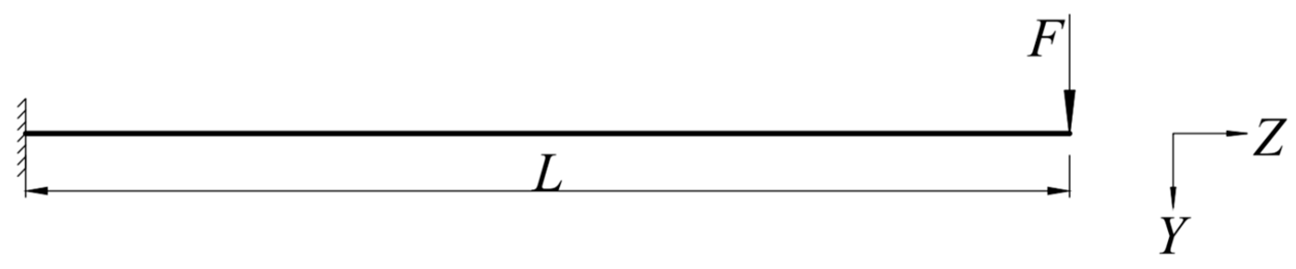
F = the concentrated load
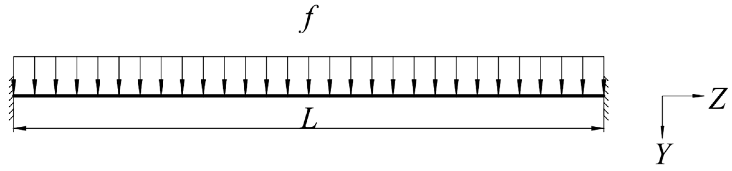
f = the uniformly distributed load
f(x) = the distribution function corresponding to the shear lag effect
G = the shear modulus
h = the height of webs
hi = the distance between the centroid of the cross section and the midplane of i-th flange
Ii = the inertial moment to the X-axis of the i-th flange
L = the length of the beam
M = the bending moment of the cross-section
Ni = the parameter related to the cross-sectional properties
O = the origin of the coordinate
Q = the cross-sectional shear force
q = the shear flow
Sx = the static moment to the X-axis
s = the curvilinear coordinates of the section profile
ti = the thickness of the i-th flange
Ui = the strain energy of the i-th flange
ui(x,z) = the longitudinal displacement of the i-th flange
V = the external load potential energy of the system
w = the vertical deflection
X = the width direction of the section
x0 = the distance from the shear flow’s zero point to the side web in the opened double-cell section
Y = the height direction of the section
Z = the longitudinal direction of the beam
γ = the shear strain
ε = the axial strain
ηi = the introduced coefficient
λ = the shear lag coefficient
μ = the Poisson’s ratio
Π = the total potential energy of the system
σ = the bending normal stress
φ(z) = the maximum difference in the shear angle
Figure 1.
Schematic of thin-walled box sections: (a) single cell; (b) double cell.
Figure 1.
Schematic of thin-walled box sections: (a) single cell; (b) double cell.
Figure 2.
Shear flow distribution of the single-cell section.
Figure 2.
Shear flow distribution of the single-cell section.
Figure 3.
Shear flow distribution of the open double-cell section.
Figure 3.
Shear flow distribution of the open double-cell section.
Figure 4.
Shear flow distribution of the closed double-cell section.
Figure 4.
Shear flow distribution of the closed double-cell section.
Figure 5.
Schematic of critical points on the box section: (a) single cell; (b) double cell.
Figure 5.
Schematic of critical points on the box section: (a) single cell; (b) double cell.
Figure 6.
Simply supported beam under concentrated load.
Figure 6.
Simply supported beam under concentrated load.
Figure 7.
Simply supported beam under uniformly distributed load.
Figure 7.
Simply supported beam under uniformly distributed load.
Figure 8.
Cantilever beam under concentrated load.
Figure 8.
Cantilever beam under concentrated load.
Figure 9.
Cantilever beam under uniformly distributed load.
Figure 9.
Cantilever beam under uniformly distributed load.
Figure 10.
ANSYS finite element model of box girders: (a) single cell; (b) double cell.
Figure 10.
ANSYS finite element model of box girders: (a) single cell; (b) double cell.
Figure 11.
Schematic of force application in the finite element model: (a) single cell; (b) double cell.
Figure 11.
Schematic of force application in the finite element model: (a) single cell; (b) double cell.
Figure 12.
Vertical displacements of Example 1. (Zhang [
17]).
Figure 12.
Vertical displacements of Example 1. (Zhang [
17]).
Figure 13.
Longitudinal distributions of shear lag coefficients of Example 1: (
a)
λ(
a11) (top plate at
x = 0 m); (
b)
λ(
a12) (top plate at
x = 3 m); (
c)
λ(
a13) (cantilever plate at
x = 5 m); (
d)
λ(
a14) (bottom plate at
x = 0 m); (
e)
λ(
a15) (bottom plate at
x = 3 m). (Zhang [
17]).
Figure 13.
Longitudinal distributions of shear lag coefficients of Example 1: (
a)
λ(
a11) (top plate at
x = 0 m); (
b)
λ(
a12) (top plate at
x = 3 m); (
c)
λ(
a13) (cantilever plate at
x = 5 m); (
d)
λ(
a14) (bottom plate at
x = 0 m); (
e)
λ(
a15) (bottom plate at
x = 3 m). (Zhang [
17]).
Figure 14.
Transverse distributions of shear lag coefficients of Example 1: (
a)
z = 20 m; (
b)
z = 18 m. (Zhang [
17]).
Figure 14.
Transverse distributions of shear lag coefficients of Example 1: (
a)
z = 20 m; (
b)
z = 18 m. (Zhang [
17]).
Figure 15.
Vertical displacements of Example 2. (Zhang [
17]).
Figure 15.
Vertical displacements of Example 2. (Zhang [
17]).
Figure 16.
Longitudinal distributions of shear lag coefficients of Example 2: (
a)
λ(
a11) (top plate at
x = 0 m); (
b)
λ(
a12) (top plate at
x = 3 m); (
c)
λ(
a13) (cantilever plate at
x = 5 m); (
d)
λ(
a14) (bottom plate at
x = 0 m); (
e)
λ(
a15) (bottom plate at
x = 3 m). (Zhang [
17]).
Figure 16.
Longitudinal distributions of shear lag coefficients of Example 2: (
a)
λ(
a11) (top plate at
x = 0 m); (
b)
λ(
a12) (top plate at
x = 3 m); (
c)
λ(
a13) (cantilever plate at
x = 5 m); (
d)
λ(
a14) (bottom plate at
x = 0 m); (
e)
λ(
a15) (bottom plate at
x = 3 m). (Zhang [
17]).
Figure 17.
Transverse distributions of shear lag coefficients of Example 2: (
a)
z = 20 m; (
b)
z = 18 m. (Zhang [
17]).
Figure 17.
Transverse distributions of shear lag coefficients of Example 2: (
a)
z = 20 m; (
b)
z = 18 m. (Zhang [
17]).
Figure 18.
Vertical displacements of Example 3.
Figure 18.
Vertical displacements of Example 3.
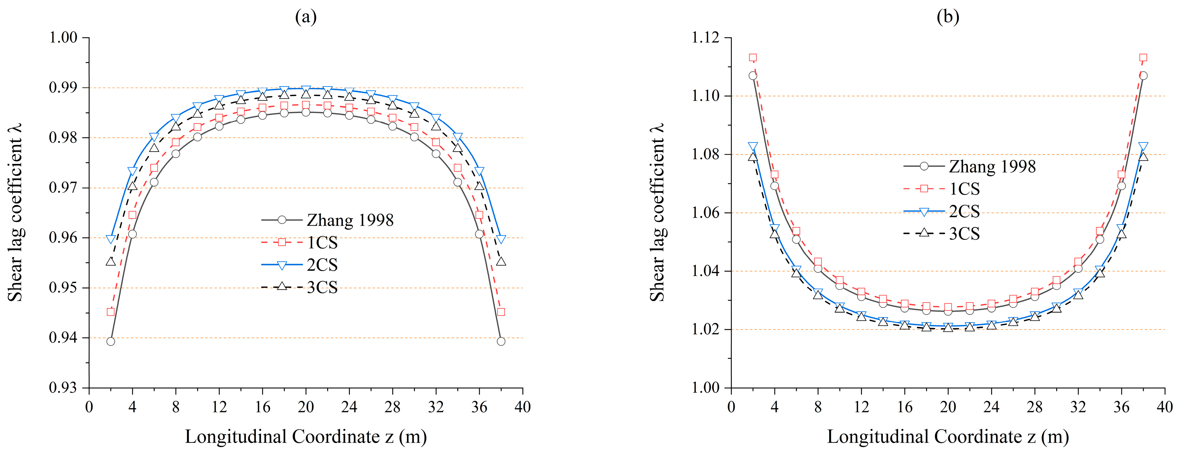
Figure 19.
Longitudinal distributions of shear lag coefficients of Example 3: (a) λ(a21) (top plate at x = 0 m); (b) λ(a22) (top plate at x = b11 m); (c) λ(a23) (top plate at x = 5 m); (d) λ(a24) (cantilever plate at x = 8 m); (e) λ(a25) (bottom plate at x = 0 m); (f) λ(a26) (bottom plate at x = b31 m); (g) λ(a27) (bottom plate at x = 5 m).
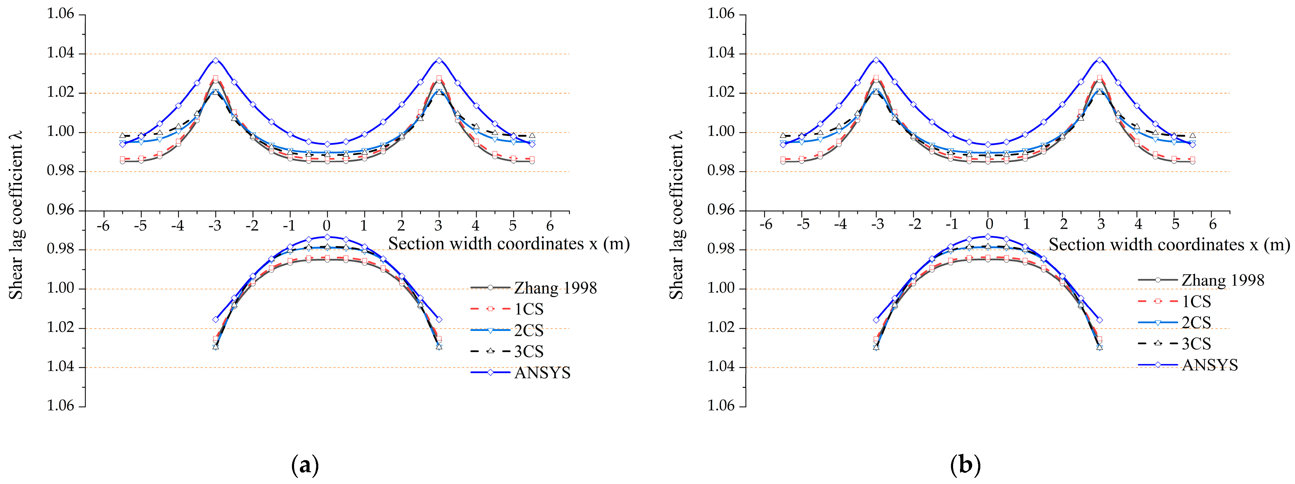
Figure 20.
Transverse distributions of shear lag coefficients of Example 3: (a) z = 20 m; (b) z = 18 m.
Figure 20.
Transverse distributions of shear lag coefficients of Example 3: (a) z = 20 m; (b) z = 18 m.
Figure 21.
Vertical displacements of Example 4.
Figure 21.
Vertical displacements of Example 4.
Figure 22.
Longitudinal distributions of shear lag coefficients of Example 4: (a) λ(a21) (top plate at x = 0 m); (b) λ(a22) (top plate at x = b11 m); (c) λ(a23) (top plate at x = 5 m); (d) λ(a24) (cantilever plate at x = 8 m); (e) λ(a25) (bottom plate at x = 0 m); (f) λ(a26) (bottom plate at x = b31 m); (g) λ(a27) (bottom plate at x = 5 m).
Figure 23.
Transverse distributions of shear lag coefficients of Example 4: (a) z = 20 m; (b) z = 18 m.
Figure 23.
Transverse distributions of shear lag coefficients of Example 4: (a) z = 20 m; (b) z = 18 m.
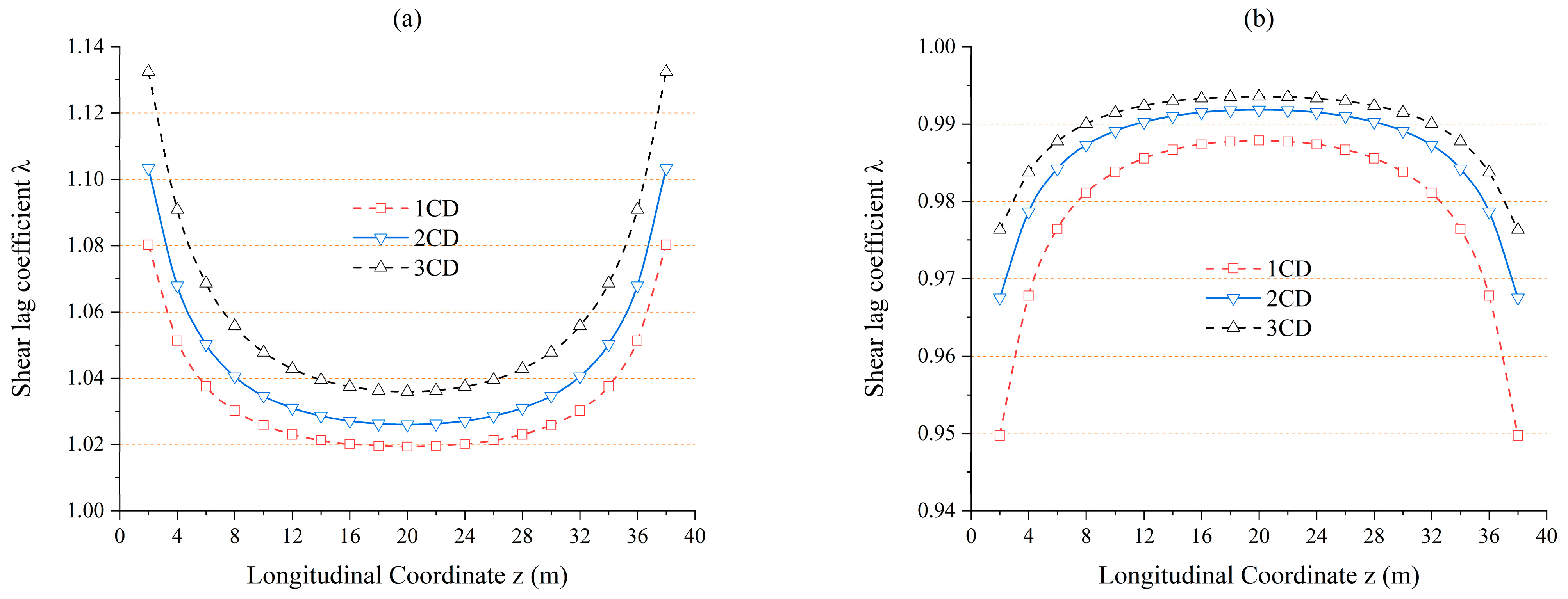
Figure 24.
Longitudinal distributions of shear lag coefficients of Example 5: (a) λ(a21) (top plate at x = 0 m); (b) λ(a22) (top plate at x = b11 m); (c) λ(a23) (top plate at x = 5 m); (d) λ(a24) (cantilever plate at x = 8 m); (e) λ(a25) (bottom plate at x = 0 m); (f) λ(a26) (bottom plate at x = b31 m); (g) λ(a27) (bottom plate at x = 5 m).
Figure 25.
Transverse distributions of shear lag coefficients of Example 5: (a) z = 2 m; (b) z = 20 m.
Figure 25.
Transverse distributions of shear lag coefficients of Example 5: (a) z = 2 m; (b) z = 20 m.
Figure 26.
Double-cell box girder fixed at both ends under uniformly distributed load.
Figure 26.
Double-cell box girder fixed at both ends under uniformly distributed load.
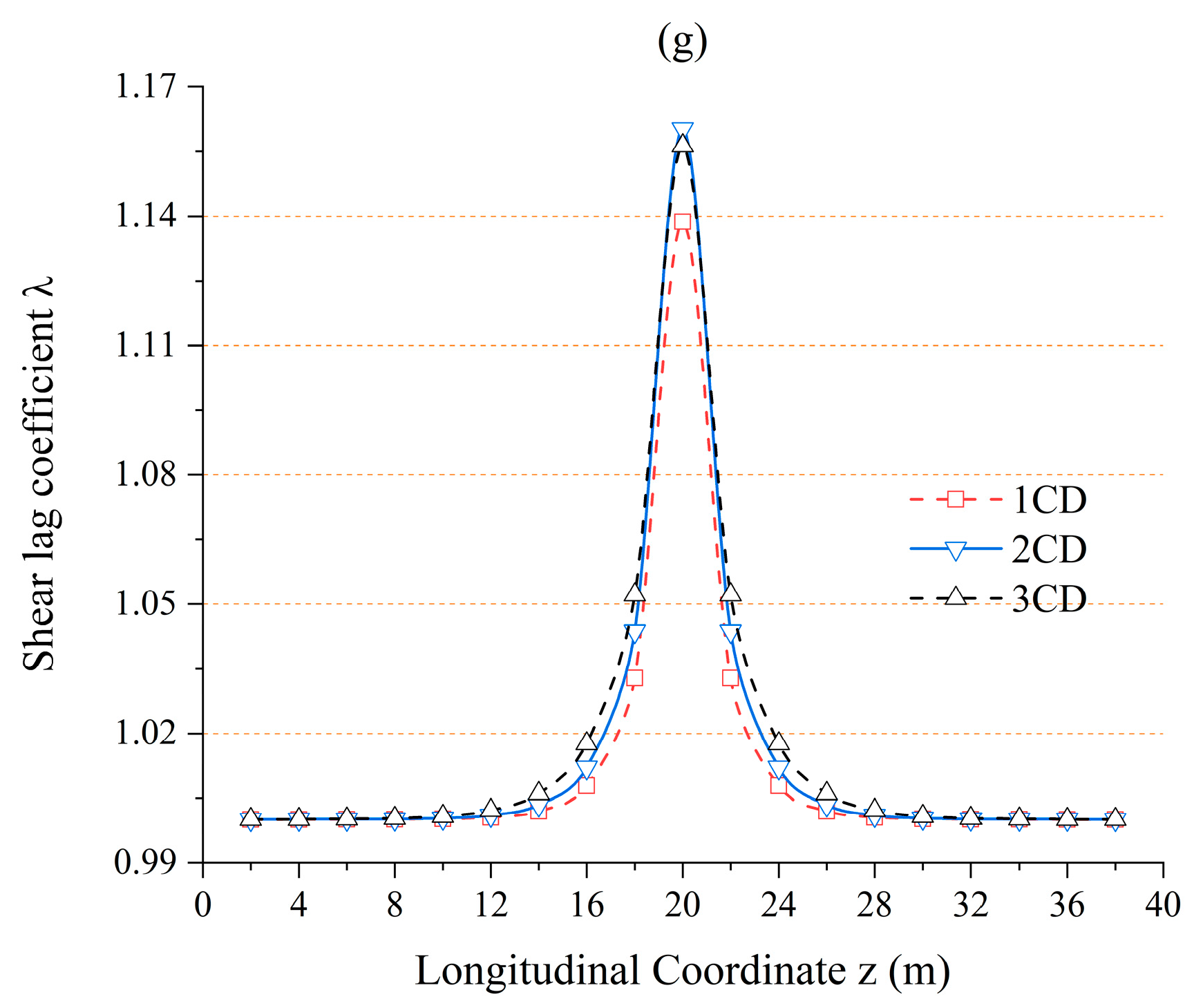
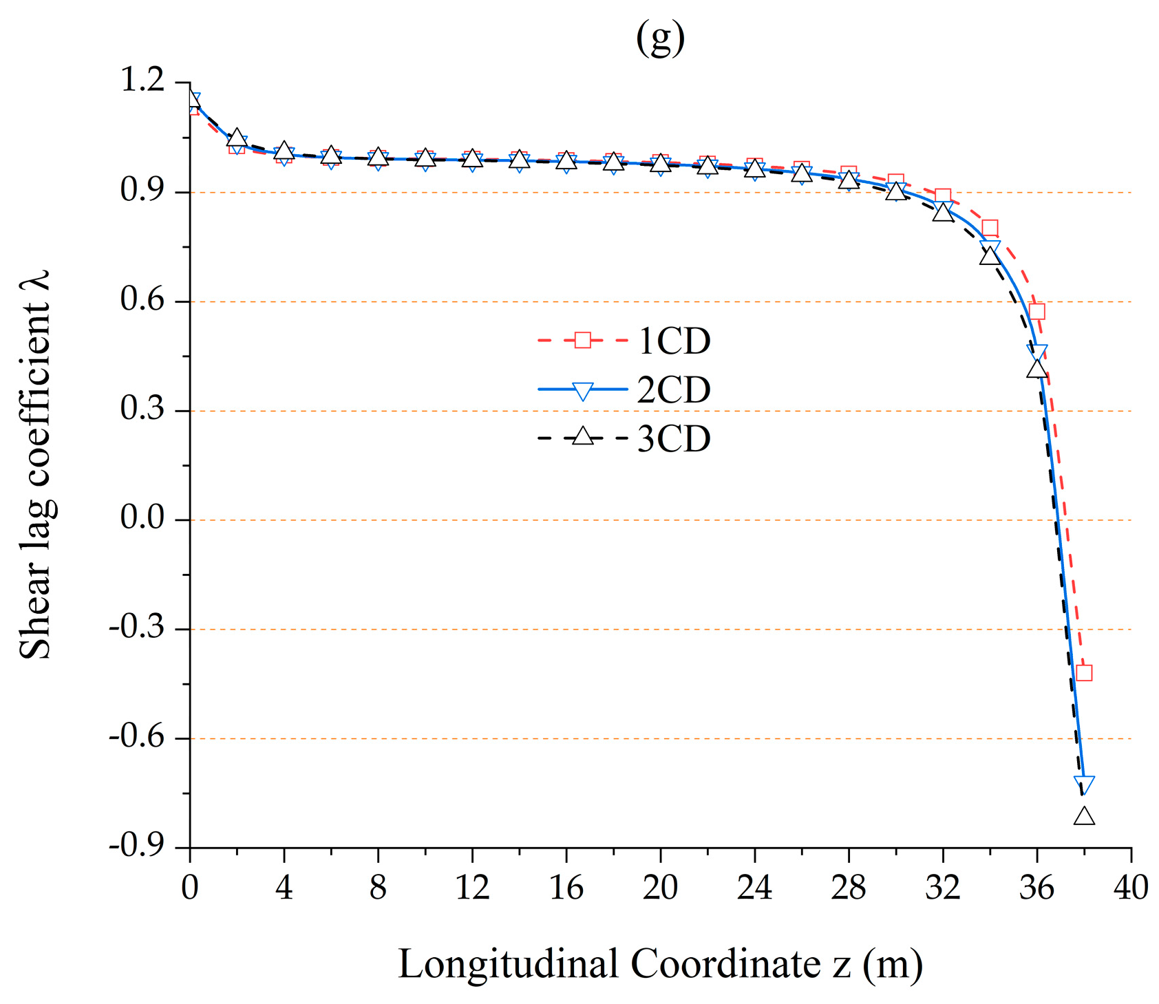
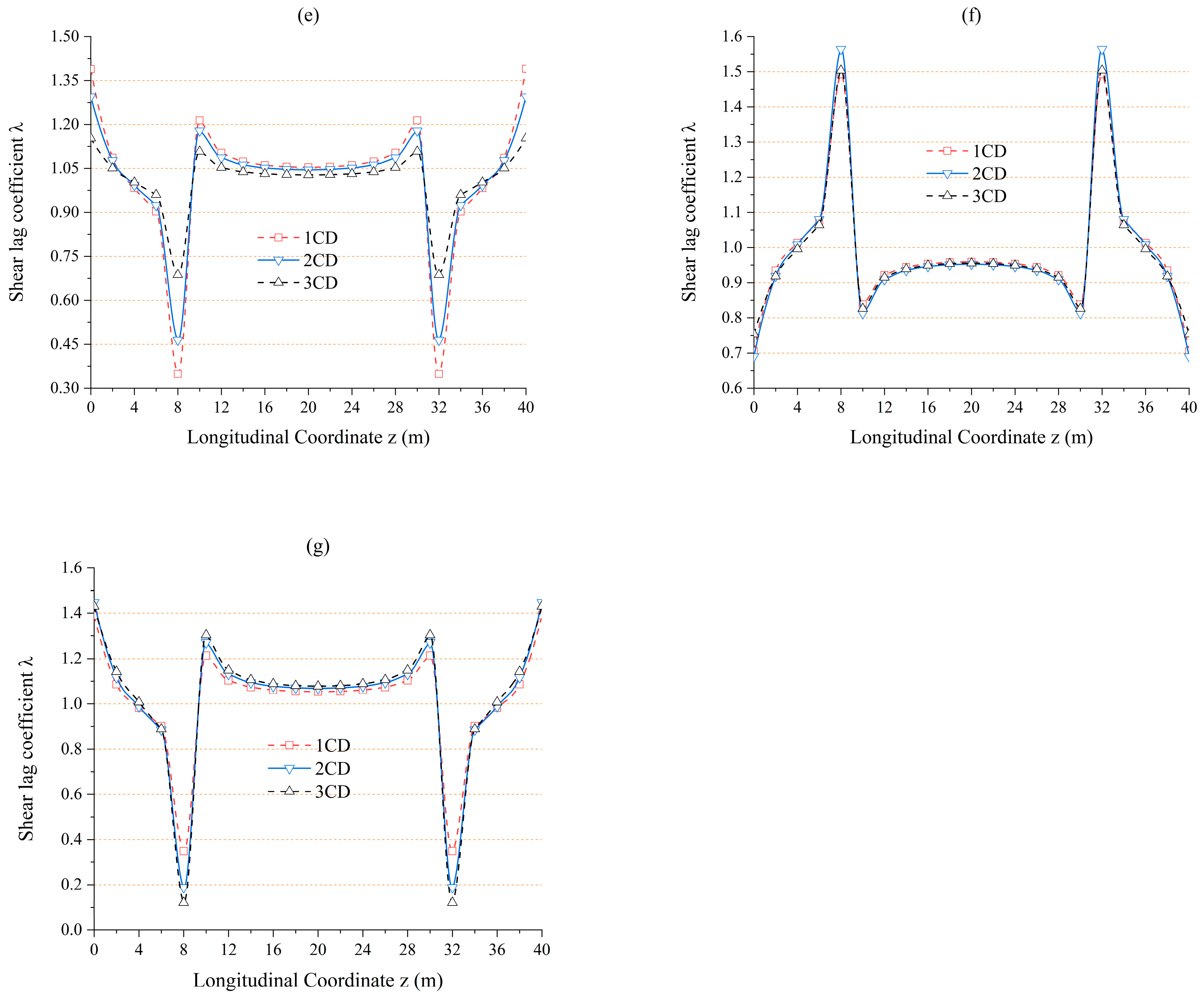
Figure 27.
Longitudinal distributions of shear lag coefficients of Example 6: (a) λ(a21) (top plate at x = 0 m); (b) λ(a22) (top plate at x = b11 m); (c) λ(a23) (top plate at x = 5 m); (d) λ(a24) (cantilever plate at x = 8 m); (e) λ(a25) (bottom plate at x = 0 m); (f) λ(a26) (bottom plate at x = b31 m); (g) λ(a27) (bottom plate at x = 5 m).
Figure 28.
Transverse distributions of shear lag coefficients of Example 6: (a) z = 2 m; (b) z = 20 m.
Figure 28.
Transverse distributions of shear lag coefficients of Example 6: (a) z = 2 m; (b) z = 20 m.
Table 1.
Shear flow magnitudes of the single-cell section at critical points.
Table 1.
Shear flow magnitudes of the single-cell section at critical points.
| points | 1 | 2 | 3 | 4-left | 4-right | 5 |
| q | 0 | t2b3h2 | 0 | −t1b2h1 | t1b1h1 | 0 |
Table 2.
Shear flow magnitudes of the closed double-cell section at critical points.
Table 2.
Shear flow magnitudes of the closed double-cell section at critical points.
| points | 1-left | 2 | 3 | 4-left | 4-right | 5 |
| q | −t2b31h2 | t2b32h2 | 0 | −t1b21h1 | t1b12h1 | −t1b11h1 |
Table 3.
Relative errors of shear lag coefficients of Example 1.
Table 3.
Relative errors of shear lag coefficients of Example 1.
| Point | ANSYS | 1CS | 2CS | 3CS | Zhang [17] |
|---|
| 20 m | 18 m | 20 m | 18 m | 20 m | 18 m | 20 m | 18 m |
|---|
| a11 | 0% | 1.04% | 0.49% | 2.29% | 0.06% | 1.44% | 0.22% | 2.20% | 0.77% |
| a12 | 2.02% | 0.37% | 3.21% | 1.40% | 3.96% | 1.54% | 1.01% | 0.62% |
| a13 | 1.16% | 0.17% | 8.61% | 1.41% | 11.07% | 2.03% | 0.02% | 0.45% |
| a14 | 0.30% | 1.722% | 2.61% | 0.57% | 2.62% | 0.46% | 1.33% | 1.93% |
| a15 | 2.05% | 1.26% | 3.32% | 2.23% | 3.15% | 2.31% | 2.71% | 1.47% |
Table 4.
Relative errors of shear lag coefficients of Example 2.
Table 4.
Relative errors of shear lag coefficients of Example 2.
| Point | ANSYS | 1CS | 2CS | 3CS | Zhang [17] |
|---|
| 20 m | 18 m | 20 m | 18 m | 20 m | 18 m | 20 m | 18 m |
|---|
| a11 | 0% | 0.75% | 0.74% | 0.42% | 0.41% | 0.56% | 0.55% | 0.90% | 0.89% |
| a12 | 0.86% | 0.85% | 1.49% | 1.50% | 1.58% | 1.59% | 1.00% | 1.00% |
| a13 | 0.73% | 0.73% | 0.12% | 0.13% | 0.43% | 0.45% | 0.88% | 0.88% |
| a14 | 1.08% | 1.08% | 0.56% | 0.55% | 0.51% | 0.51% | 1.20% | 1.20% |
| a15 | 0.95% | 0.95% | 1.38% | 1.38% | 1.40% | 1.40% | 1.06% | 1.06% |
Table 5.
Relative errors of shear lag coefficients of Example 3.
Table 5.
Relative errors of shear lag coefficients of Example 3.
| Points | ANSYS | 1CD | 2CD | 3CD |
|---|
| 20 m | 18 m | 20 m | 18 m | 20 m | 18 m |
|---|
| a21 | 0% | 0.40% | 4.64% | 3.27% | 3.32% | 6.21% | 1.26% |
| a22 | 4.38% | 3.51% | 0.53% | 2.86% | 1.44% | 2.59% |
| a23 | 2.20% | 2.37% | 0.43% | 2.62% | 2.15% | 2.54% |
| a24 | 9.92% | 7.56% | 5.48% | 6.09% | 2.55% | 3.51% |
| a25 | 9.70% | 1.80% | 6.53% | 1.41% | 1.70% | 0.40% |
| a26 | 1.99% | 0.60% | 2.68% | 1.16% | 0.31% | 1.11% |
| a27 | 2.40% | 4.59% | 0.55% | 3.59% | 0.88% | 2.81% |
Table 6.
Relative errors of shear lag coefficients of Example 4.
Table 6.
Relative errors of shear lag coefficients of Example 4.
| Points | ANSYS | 1CD | 2CD | 3CD |
|---|
| 20 m | 18 m | 20 m | 18 m | 20 m | 18 m |
|---|
| a21 | 0% | 3.20% | 3.22% | 2.57% | 2.59% | 1.63% | 1.63% |
| a22 | 2.34% | 2.35% | 1.94% | 1.96% | 1.77% | 1.78% |
| a23 | 1.02% | 1.02% | 1.23% | 1.24% | 1.27% | 1.27% |
| a24 | 2.68% | 2.77% | 2.01% | 2.09% | 0.88% | 0.95% |
| a25 | 0.98% | 0.98% | 0.69% | 0.69% | 0.12% | 0.11% |
| a26 | 0.63% | 0.63% | 0.86% | 0.87% | 0.76% | 0.77% |
| a27 | 1.92% | 1.93% | 1.45% | 1.46% | 1.15% | 1.15% |
Table 7.
Relative errors of shear lag coefficients of Example 5.
Table 7.
Relative errors of shear lag coefficients of Example 5.
| Points | ANSYS | 1CD | 2CD | 3CD |
|---|
| 2 m | 20 m | 2 m | 20 m | 2 m | 20 m |
|---|
| a21 | 0% | 1.52% | 1.34% | 0.32% | 2.01% | 1.55% | 3.01% |
| a22 | 2.04% | 1.72% | 1.50% | 2.10% | 1.27% | 2.27% |
| a23 | 1.37% | 2.64% | 1.56% | 2.41% | 1.47% | 2.38% |
| a24 | 8.21% | 5.91% | 6.93% | 5.31% | 4.69% | 4.30% |
| a25 | 3.52% | 3.16% | 3.20% | 2.87% | 2.33% | 2.30% |
| a26 | 0.16% | 1.51% | 0.65% | 1.29% | 0.63% | 1.39% |
| a27 | 0.11% | 0.34% | 1.04% | 0.83% | 1.77% | 1.15% |
Table 8.
Relative errors of shear lag coefficients of Example 6.
Table 8.
Relative errors of shear lag coefficients of Example 6.
| Points | ANSYS | 1CD | 2CD | 3CD |
|---|
| 2 m | 20 m | 2 m | 20 m | 2 m | 20 m |
|---|
| a21 | 0% | 1.22% | 4.38% | 2.43% | 2.57% | 8.17% | 0.12% |
| a22 | 3.70% | 2.86% | 2.02% | 1.67% | 1.33% | 1.14% |
| a23 | 0.93% | 0.35% | 0.44% | 0.30% | 0.81% | 0.40% |
| a24 | 36.72% | 13.41% | 31.35% | 11.14% | 21.79% | 7.31% |
| a25 | 13.51% | 4.59% | 12.57% | 3.73% | 9.79% | 2.00% |
| a26 | 2.72% | 0.13% | 0.95% | 0.85% | 0.92% | 0.55% |
| a27 | 2.51% | 3.76% | 0.26% | 2.42% | 2.53% | 1.55% |


