Article

The Structural Design and Optimization of Top-Stiffened Double-Layer Steel Truss Bridges Based on the Response Surface Method and Particle Swarm Optimization

1
Highway School, Chang’an University, Xi’an 710064, China
2
Key Laboratory of Transport Industry of Bridge Detection Reinforcement Technology, Chang’an University, Xi’an 710064, China
3
School of Civil Engineering, Chongqing University, Chongqing 400045, China
*
Author to whom correspondence should be addressed.
Appl. Sci. 2023, 13(19), 11033; https://doi.org/10.3390/app131911033
Submission received: 28 August 2023 / Revised: 26 September 2023 / Accepted: 5 October 2023 / Published: 7 October 2023
(This article belongs to the Special Issue Bridge Structural Analysis)

Abstract

:
A lightweight design optimization algorithm is proposed to optimize the design parameters of stiffened double-layer steel girder bridges, the aim of which is to improve structural safety and reduce superstructure works. Taking a top-stiffened double-layer steel truss bridge as the reference project, a multiscale mixed-element model of the initial design parameters is established, and its computational accuracy is verified. Considering the structural configuration and loading characteristics of the bridge, the elastic modulus of steel, the deck plate thickness, the stiffening vertical bar height, and the relative distance between the double-layer main girders are selected as the design parameters for optimization. The mid-span vertical deflection, the axial forces in the stiffeners, the bottom plate of the deck, the compressed web tube at the pier top, and the quantity of superstructure works are chosen as the objective functions to be minimized. A lightweight calculation equation reflecting the relationship between the optimization parameters and the objective functions is established using the response surface method (RSM). Subsequently, an improved weighted particle swarm optimization (WPSO) model is employed to perform the multi-objective optimization of the design parameters for the bridge, and the results are compared with those obtained from the multi-objective genetic algorithm NSGA-II. The results show that the RSM accurately fits the numerical relationship between the optimization parameters and the objective response functions. When minimizing the quantity of superstructure works as the primary control objective and minimizing the mid-span vertical deflection and the axial forces in the compressed web tube at the pier top as secondary control objectives, the optimization results achieved by WPSO outperform those obtained by NSGA-II. The optimized results lead to reductions of 11.09%, 3.92%, 7.56%, 4.45%, and 8.38% in the respective objective function values of the structure. This method has important theoretical significance for the optimization of structural design parameters.

1. Introduction

With the rapid expansion of the urban environment and the fast advancement of economic construction, steel truss bridges are favored because of their light weight, high strength, and strong adaptability [1]. However, while steel truss bridges are widely used as long-span bridges, the increasing vehicle load also brings new challenges to their structural design. Bridge structure design optimization seeks the functional relationship between the design parameters and output responses to achieve one or more of the goals of reducing bridge construction costs, improving structural bearing safety and stability, improving structural durability, and enhancing construction environmental protection. In the context of economic globalization, structural design optimization can improve the existing design level, reduce construction costs, and increase the core competitiveness of bridges with similar structural designs.
Finite element (FE) modeling methods are generally used for traditional steel truss bridge design and verification calculations. However, when performing multi-parameter optimization, it is necessary to manually adjust various parameter combinations to perform trial calculations and verify the optimization results; in particular, for large-scale bridge models with a large number of meshes and complex structures, the optimization process will be slow and will consume large amounts of computing time and resources. Therefore, under the current situation, namely, the daily increase in the number of long-span steel truss bridges and the increasingly more stringent optimization requirements of bridge design, it is necessary to find a lightweight multi-parameter design optimization algorithm.
At present, the commonly used bridge optimization methods mainly include mathematical optimization methods, structural optimization methods based on empirical equations, deep learning methods [2], etc. Mathematical optimization methods can be used to solve multi-constraint and nonlinear problems, but they require numerous calculations, take a long amount of time, and sometimes cannot converge to the global optimal solution. Structural optimization methods based on empirical equations have a simple calculation process and quickly yield results, but the dependent empirical equation may not completely match the actual structure, resulting in low-precision results. Finally, although deep learning methods can provide high-precision calculation results, they require a large amount of sample data for training, and the time cost is high. In contrast, the response surface method (RSM) can explicitly express the optimization function; it has the characteristics of a concise form, clear logic, and rapid response, and is suitable for the lightweight design of long-span complex structures. It maps each point in the design space to the value of each design variable, establishes a response surface based on the overall response of the design target, and then optimizes the structural design parameters by analyzing the response surface.
In recent years, scholars have carried out detailed research on the application of the RSM in civil engineering. The extant literature has mainly focused on the local components (mainly simply supported beams), the damage identification of girders [3,4], bridge piers [5], and stay cables [6], and the seismic design of bridges with simple structures [7,8,9]. Moreover, the results of load tests have been used to correct the FE models of bridges undergoing service modification [10,11,12,13,14], and the experimental design method has been adopted to study the mechanical properties of new building materials [15]. The design parameter adjustment method has also been used to study the mechanical properties of structures [16,17], and construction monitoring data have been utilized to monitor and control the construction process [18]. However, there have been few related studies on the multi-objective optimal design of bridges using the RSM. In addition, the extant optimization research on bridge structures has primarily focused on simple structures, and there is limited research on the optimization of large-span bridges with complex structures.
The engineering project considered in this study is a complex large-span double-layer steel truss bridge, for which traditional optimization methods would result in significant time and economic costs. A new optimization method is proposed to achieve rapid and accurate structural design optimization for this complex bridge. First, a multiscale hybrid element model of the bridge is established using ABAQUS FE software (https://www.3ds.com/products-services/simulia/products/abaqus/) based on the de-sign drawings. Next, the RSM is used to fit the model data and extract sensitive parameters via significance analysis. This leads to the formulation of a lightweight equation for structural variables, which takes into account the elastic modulus of steel, the bridge deck thickness, the maximum length of the stiffening vertical rods, and the relative distance between the double-layer main beams. Based on this, a multi-objective optimization algorithm with the response function as the control indicator is adopted to find an optimized solution that maximizes the structural load-bearing capacity while minimizing material costs, such as achieving the minimal vertical deflection of the structure while minimizing the engineering quantity of the upper structure. (The minimization of material costs mentioned in this article generally refers to minimizing the amount of upper structure engineering).

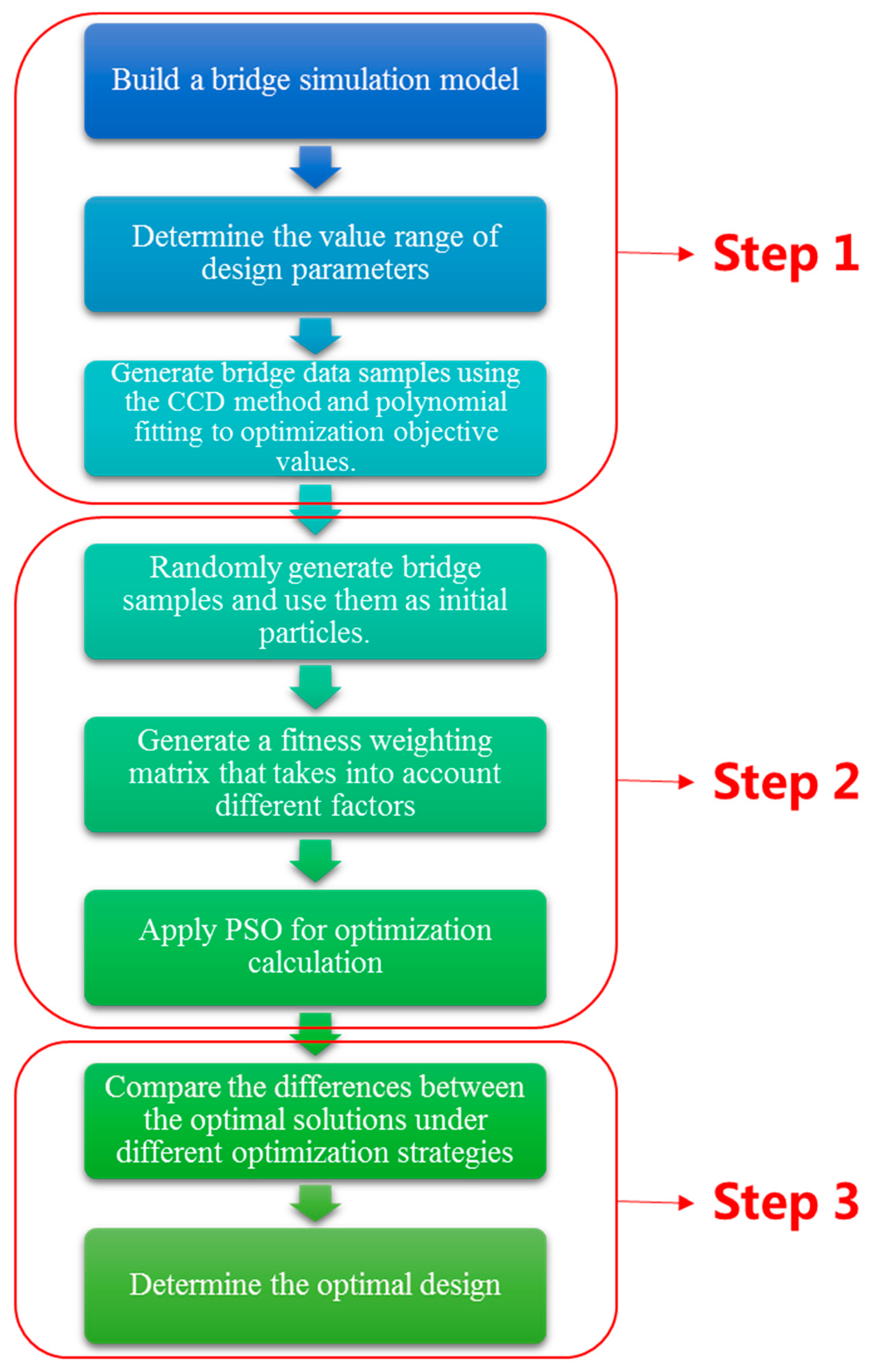
2. Capacity Optimal Design Method

2.1. Response Surface Method
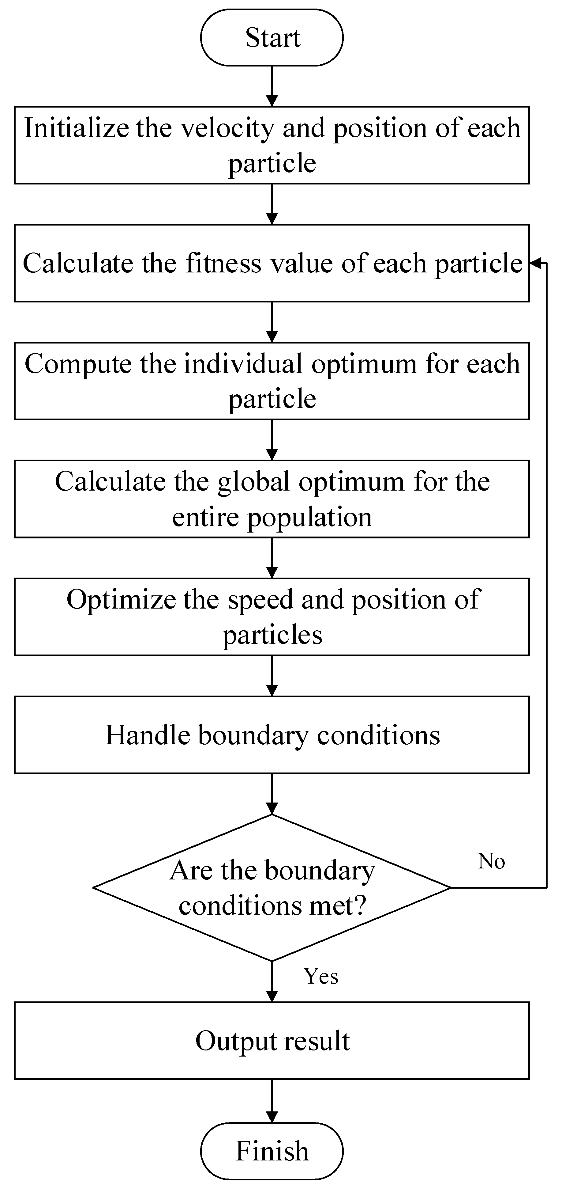
As a statistical method, the RSM can establish a predictive model via multiple nonlinear regression. The RSM is widely used as an alternative model in parameter sensitivity analysis and design optimization to improve the computational efficiency. The RSM assumes that the response of the structure can be approximated as
Z = n i = 1 k i φ i ( x ) ,
where Z is the structural response, φ i ( x ) is the basis function, n is the number of basic functions, and k i is the response function coefficient.
According to the least-squares method, the response surface function coefficient is determined as
K = Φ T Φ 1 Φ T Z ,
where K is the response surface function coefficient matrix, K = [ k 0 , k 1 , , k n ] . Moreover, Φ is the matrix formed by the sample points and is expressed as follows:
Φ = φ 1 x ( 1 ) φ n x ( 1 ) φ 1 x ( i ) φ n x ( i ) φ 1 x ( m ) φ n x ( m ) .
The response surface function Z can be obtained by solving the matrix equation of the random variables of the response surface to find the response surface function coefficient. For most engineering problems, Z is represented as a second-order polynomial function with cross-terms to take into account the linearity, interaction, and curvature linear terms.
Z = a 0 + c i = 1 a i x i + c i = 1 a i i x i 2 + c i = 1 c j > i a i j x i x j ,
where a 0 is the constant coefficient of the response surface, a i is the coefficient of the linear term of the response surface, a i i is the coefficient of the quadratic term of the response surface, a i j is the coefficient of the interaction term of the response surface, and c is the number of design parameters.

2.2. WPSO

Particle swarm optimization (PSO) is derived from the simulation of bird predation. In essence, it is a random search algorithm suitable for finding the optimal solution in a dynamic and multi-objective optimization environment.
The search space of optimization problems is analogous to the flight space of birds, each of which is abstracted into a particle without mass and volume, which is used to represent a possible solution to all problems. Each group of particles begins by randomly assigning an initial position x and initial velocity v in a given space, and x and v are then updated using the following equations:
v i j ( t + 1 ) = w · v i j ( t ) + c 1 r 1 ( t ) p i j ( t ) x i j ( t ) + c 2 r 2 ( t ) p g i ( t ) x i j ( t ) ,
x i j ( t + 1 ) = x i j ( t ) + v i j ( t + 1 ) ,
where t is the current iteration number, r 1 and r 2 are distributed in [0, 1], and p i j ( t ) is the historical optimal position of the i-th particle. Moreover, p g i ( t ) is the best historical group position, and c 1 and c 2 are non-negative constants. The velocity and position are usually limited to a certain interval, namely, [ v m a x , v m a x ] and [ x m a x , x m a x ] , respectively. Finally, w is the dynamic iteration weight, which is adopted as the following decreasing linear equation:
w = w max w max w min · t T max ,
where T m a x represents the maximum number of evolutions, and w m a x and w m i n , respectively, denote the maximum and minimum inertia weight values.
The fitness values f i t [ i ] for each particle are calculated to select the individual extremum p b e s t ( i ) for the i-th iteration and the global extremum g b e s t ( i ) among all iterations. When the algorithm termination condition is satisfied, the global extremum and the corresponding position are the optimal results.
When actual engineering problems involve the constrained optimization of complex multi-objective functions, a fitness function with a fixed value often cannot achieve the expected results. In this case, the optimization problem is usually solved by the improved weighted PSO (WPSO) method. In this algorithm, the fitness function is often not a single function, but a multifunctional equation system. The fitness-weighted matrix f i t [ i ] · η i 2 is introduced into the Euclidean norm equation of the fitness function, which sorts the function priority and can be represented as follows:
f i t [ i ] · η i 2 = f i t [ x i 1 ] · η i 1 2 + f i t [ x i 2 ] · η i 2 2 + + f i t [ x i n ] · η i n 2 1 / 2 ,
where f i t [ x i j ] ( j = 1 ~ n ) represents each desirable equation for the optimization function, and η i j ( j = 1 ~ n ) represents the importance weight of each desirability equation.
In this case, f i t [ i ] · η i 2 is the desirability function for the actual optimization of the system of equations. The RSM and WPSO are integrated to design the WPSO-RSM model.

2.3. Decision-Making

WPSO can be used to obtain a series of Pareto solutions, including both the global optimal solution and suboptimal solutions. However, based on practical considerations, it is necessary to select a single preferred solution from the Pareto solutions. Therefore, to select the most suitable optimization solution from multiple options in accordance with engineering practicality, the following three different optimization strategies are considered.
Strategy I: Prioritize increasing the load-bearing capacity of the bridge structure without increasing the material costs. This strategy is generally applicable to bridges that require further improvement in the load-bearing capacity and the material utilization rate of the upper structure.
Strategy II: Prioritize minimizing the material costs while ensuring that the load-bearing capacity of the bridge structure is not reduced. This strategy is generally applicable to bridges with sufficient safety reserves for which costs must be saved to a certain extent. Scholars have previously applied this strategy to bridge optimization [19,20].
Strategy III: Prioritize achieving a balance between the load-bearing capacity and material costs of the bridge structure. This strategy is an equilibrium strategy and needs to be selected in consideration of the actual situation.
These three optimization strategies are proposed based on practical engineering experience and focus on the internal forces of the key components and the engineering quantity of the upper structure of the bridge. Considering the engineering application context of this study, Strategy II is chosen as the basis for selecting the optimal optimization solution. The optimization design process based on the WPSO-RSM model is illustrated in Figure 1, and it mainly consists of the following three steps.
Step 1: Develop the capacity response surface model.
A set of bridge samples is generated using the central composite design (CCD) method after determining the ranges of different design parameters. Then, the capacity-related values of bridge samples are subjected to polynomial fitting to determine the model parameters, which can be applied to determine the capacity response surface model by adjusting the polynomial form.
Step 2: Obtain the Pareto optimal solutions.
The bridge samples are randomly generated and considered the initial particles. Considering the material cost, the bearing capacity, and the determined constraint conditions, the fitness-weighted matrix is introduced as a Euclidean norm equation, which can be applied to sort the function priority of fitness functions. Considering the specific optimization strategies, WPSO with the determined parameters is applied to obtain the Pareto optimal solutions.
Step 3: Determine the optimal design scheme.
The final optimal design scheme can be achieved by comparing the differences in the Pareto optimal solutions of the three optimization strategies.

3. Bridge Case Study

3.1. FE Modeling

A top-stiffened steel truss bridge comprising nine main trusses with a span arrangement of 124 m + 132 m + 132 m + 168 m + 300 m + 168 m + 132 m + 132 m + 124 m was selected as a case study, as shown in Figure 2. The bridge had two layers; the upper layer was a six-lane road, and the lower layer was a four-lane road and two-track railway. Sidewalks on both sides were also cantilevered on the lower layer. Two upper stiffening rods were arranged in the middle three spans.
The horizontal chords were box-shaped cross-sectionally, the web members were h-shaped cross-sectionally, the bridge slabs were orthotropic, the upper stiffening rods were rectangle-shaped cross-sectionally, and the booms consisted of parallel steel wires. The substructure included two abutments and eight piers. W1 and W10 were joint piers, which combined an upper road pier and a lower rail pier. The others were hollow piers with 6 × 8-m rectangular sections. The upper stiffening rods were made of Q420q steel, the booms were made of Q370q steel, and the truss members were made of Q500q steel. The elastic modulus of all steel materials was 206 GPa, and the mass density was 7850 kg/m3. The concrete strength of the substructure was 45 MPa and the mass density was 2500 kg/m3. Moreover, PETE elastomeric bearings were installed at the top of each bridge pier. The cross-section arrangement of the pier cap beam and the standard main beam are shown in Figure 3.
ABAQUS software was applied to develop the nonlinear FE model of this bridge, which is presented in Figure 4. The pier top and mid-span were selected as the most important parts of the structure with the minimum remaining life. Based on the consideration of the safety of the entire structure, the remaining life of this part determines the remaining life of the whole bridge. The refined models of the small-scale segments were built by S4R shell elements, while the large-scale models of the other main beam segments were built by B31 truss elements. The shell and truss elements were assembled by the “coupling” command.
To avoid the influence of the Saint Venant effect, the modeling length of the beam element in the non-test area was appropriately lengthened so that the distance between the test section and the coupling surface was more than three times the chord section size. In practice, sliding supports are used at all piers, so only vertical displacement constraints were used for simulation, and the mesh size of the whole bridge was about 500 mm.
During bridge operation, the vehicle load will produce an uneven surface load on the bridge slab. Considering the refined analysis requirement, bridge slabs were also built by S4R shell elements. The global mesh size of the slabs was about 300 mm, and that near the upper chord was reduced to 100 mm. There were at least four layers of the elements along the thickness direction of the bridge slab.
To accurately simulate the actual force state of the longitudinal and transverse stiffened beams interacting with the bridge slab, different connection strategies were developed. Near the pier top and mid-span, S4R shell elements were used to establish longitudinal and transverse stiffener beams, while the slab and top chord were connected by Boolean operations. In the other main beam areas, B31 truss elements were used to establish longitudinal and transverse stiffener beams, while the connection between the slab and top chord was assumed to be strong enough and the “MPC” (multipoint constraint) command was applied on the interface between them.

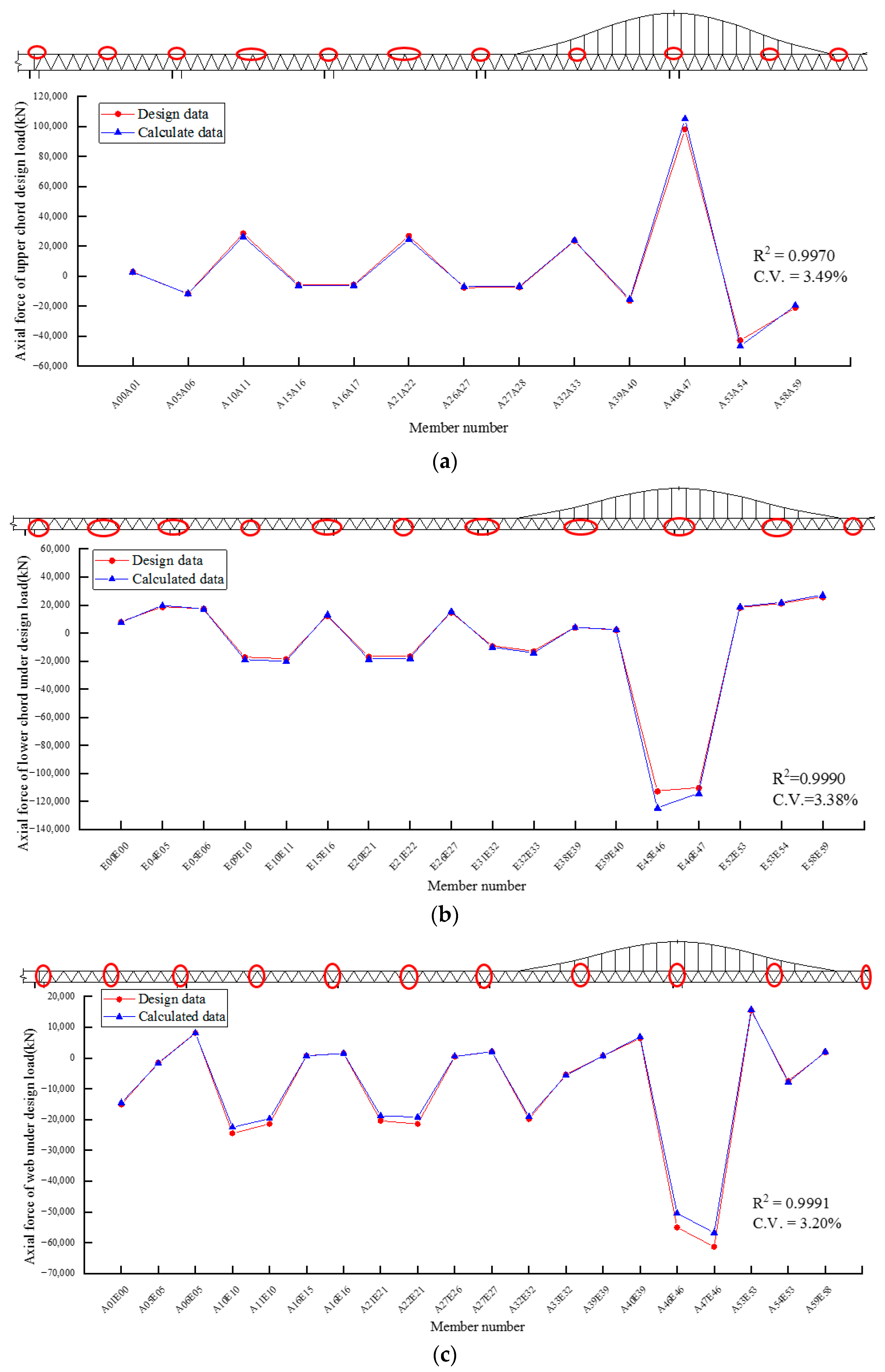
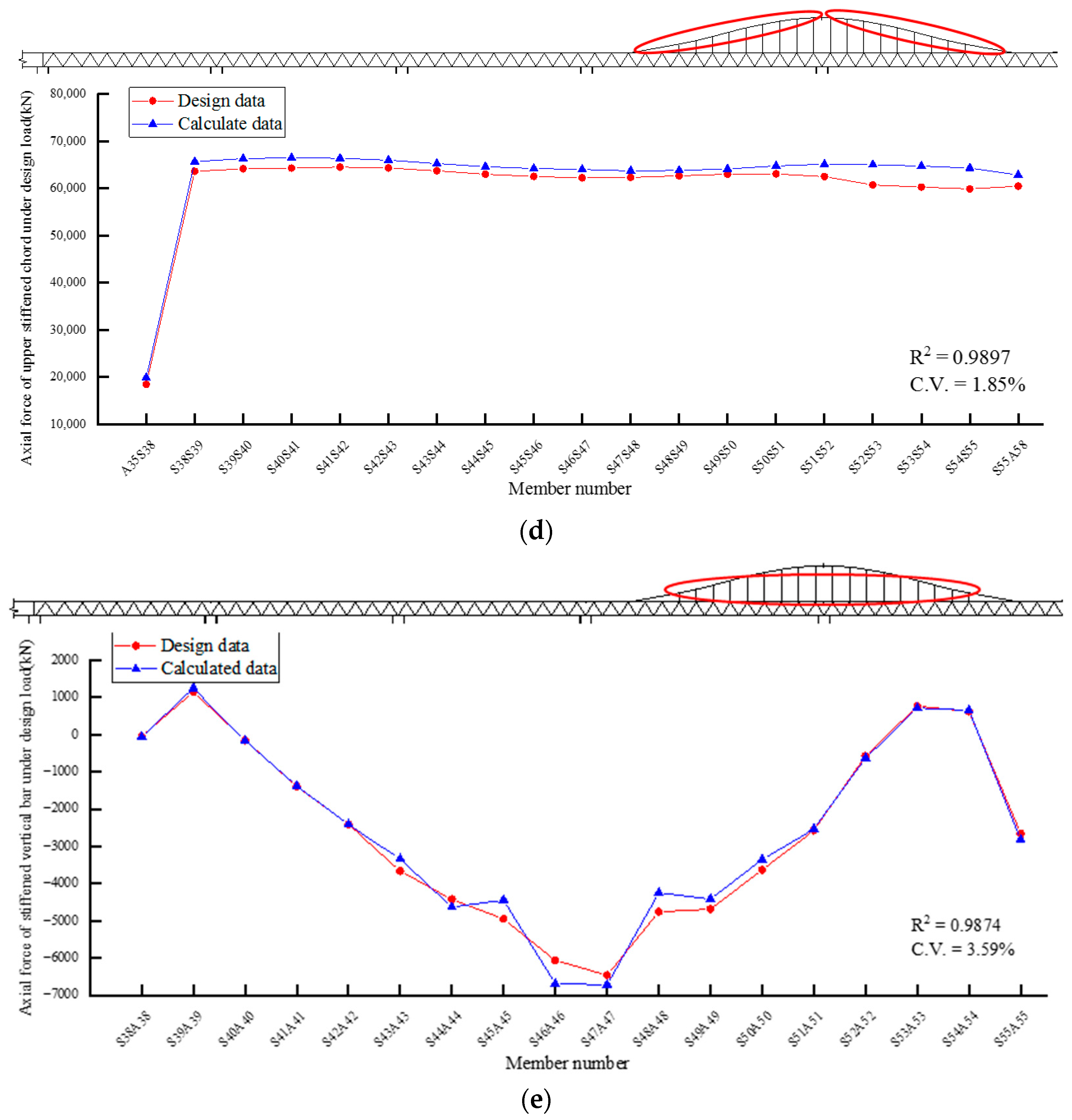
3.2. Verification of FE Modeling

To ensure the calculation accuracy of the multi-scale FE model, the calculated axial forces of the upper chord, lower chord, inclined bar, upper stiffening chord, and vertical stiffening bar under the design load were compared with the design data. The design data presented in the figure were all derived from the engineering design drawings. Due to space limitations, only the partial comparison results of the pier tops and mid-span areas in a half-span symmetrical structure are presented. In Figure 5, the position of the bar corresponding to each bar number is indicated by a red circle.
From Figure 5, it can be seen that the value of each regional component in the design data and the calculation results of the ABAQUS multi-scale mixed unit model is above 0.97, and the coefficient of variation (C.V.) is less than 4%. This demonstrates that the results generated by the ABAQUS model are stable, reliable, and in good agreement with the design data, and the calculation results can meet the precision requirements.

4. Model Lightweight Algorithm

4.1. Choice of Optimization Parameters and Objective Function

The double-layer steel truss bridge structure is complex and involves a large engineering volume. It is necessary to optimize the relevant parameters that affect the structural stress and engineering volume within a reasonable range while meeting the specifications.
The improvement of the performance of steel is an important direction for the future development of steel bridges [21]. The elastic modulus of steel, an important parameter reflecting its mechanical properties, can be optimized within a reasonable range to improve the structural stress performance and deformation. The elastic modulus of various steels at room temperature is mostly between 1.9 × 10⁵ and 2.2 × 10⁵ MPa [22]. The optimization ranges of the elastic modulus of steel described in this article include those of the steel used in the upper and lower main girders of the steel truss in the project, as well as the steel used in the bridge deck, bracing chords, and vertical stiffening bars. The parameter optimization ranges are considered to be within ±5%.
Orthotropic bridge decks consist of bridge panels, transverse ribs, and longitudinal ribs. Studies have shown that appropriately increasing the thickness of the bridge panel can improve the stress state of the orthotropic bridge deck [23], but it will increase the engineering volume. Therefore, considering the bridge panel thickness as an optimization parameter has significant engineering significance, and the parameter optimization range is considered to be within ±20%.
In the double-layer steel truss bridge with upper bracing chords, the maximum length of the vertical stiffening bars is an important parameter for structural stress, and its optimization can provide guidance for practical engineering. The relative distance be-tween the double-layer main girders is mainly determined based on the structural stiff-ness and overhead clearance requirements. Its value affects the structural stress and steel consumption, so it needs to be optimized. The design parameters of similar structures are compared with the maximum length of the vertical stiffening bars and the relative distance between the double-layer main girders of the supported project [24,25,26], and the parameter optimization range is determined within ±10%.
Based on the preceding analysis, the final selection includes four structural parameters for optimization: the elastic modulus of steel, the bridge panel thickness, the maxi-mum length of the vertical stiffening bars, and the relative distance between the double-layer main girders. The parameters to be optimized and their ranges are listed in Table 1.
To reflect the stress and deformation characteristics of the main load-bearing members in a top-stiffened steel truss bridge, several objective functions were selected for correction. These functions include the mid-span vertical deflection, the axial internal force of stiffened strings, the longitudinal internal force of the bridge deck bottom plate, and the axial internal force of the empty tube of the web bar under compression at the pier top. To ensure the accuracy of the values, each model member in the most unfavorable area was divided into five segments for calculation, and the average value was taken as the benchmark data for analysis, as reported in Table 2.
Based on the characteristics of the optimization parameters and objective function, the CCD method was employed to establish 30 sets of experimental conditions for two-level four-factor optimization parameters and objective functions. The aim was to analyze the level of sensitivity of the structural optimization parameters to the objective function while solving the contradiction between ensuring the fitting accuracy and controlling the experimental cost when using the RSM instead of a model. It is particularly important to select limited and highly representative sample data without affecting the computational accuracy. The specific experimental conditions are presented in Figure 6. The percentage shown in the figure represents the value levels of each factor under different operating conditions.

4.2. Response Surface Analysis Fitting and Precision Testing

If there are too few provided parameter points or selection errors in the experimental design; the estimated model terms may be confounded in later analysis. Therefore, considering the interaction effects of the two factors, it is important to first determine whether the selected design can sufficiently estimate the coefficients of the desired model, as shown in Table 3.
From Table 3, it can be seen that regardless of considering a single factor or the interaction effects of two factors, the estimated standard deviation of the same type of coefficient is highly similar. The variance inflation factors are 1.0 and 1.05, indicating that there are good orthogonal relationships between the selected parameters to be optimized. This satisfies the correlation between the regression coefficients, and the influence of each independent variable and the target variable can be accurately estimated and explained. Thus, the prediction effect will be more reliable and accurate. After comparison, it was found that the probability calculation of the model with a standard deviation of 2.0 is superior to those with standard deviations of 0.5 and 1.0. Therefore, a quadratic polynomial was chosen for data regression. Due to space limitations, only the response surface results of the five objective functions for parameters A and B are presented in Figure 7.
The significance of optimization parameters A–D to target functions R1R5 to be corrected was analyzed using the F-test method. Assuming the model contains m parameters, the statistical variance was calculated to ensure the significance of (m + 1) parameters.
F m + 1 = S m S m + 1 / η m η m + 1 S m + 1 / η m + 1 ,
where S m and S m + 1 are the sum-of-squares errors in the response surface equation for the m-th parameter and the (m + 1)-th parameter, respectively, and η m and η m + 1 are the degrees of freedom for the m-th parameter and the (m + 1)-th parameter, respectively.
The criterion for the significance test of the parameters is as follows: given a significance level α, when F m + 1 > F 1 α ( 1 , n m 1 ) , the (m + 1)-th parameter has higher significance and should be included in the response surface model; otherwise, it will be removed.
According to Table 3, considering the present experiment with m = 4 independent variables and n = 30 experimental runs, the F-test critical value is F α = 0.01 = 4.018 at the significance level of α = 0.01. Notably, given the substantial differences in the F-test values that correspond to each response surface of the objective functions, it is imperative to individually normalize the R1R5 single factors, the interaction factors, and their quadratic coupling terms to gain an intuitive understanding of the significance characteristics of each parameter. In this context, the F-test critical values for R1R5 are, respectively, F R 1 ( α = 0.01 ) = 7.85 × 10 3 , F R 2 ( α = 0.01 ) = 2.91 × 10 3 , F R 3 ( α = 0.01 ) = 1.88 × 10 2 , F R 4 ( α = 0.01 ) = 2.77 × 10 4 , and F R 5 ( α = 0.01 ) = 3.71 × 10 6 , and their respective levels of significance are shown in Figure 8.
It can be seen from Figure 8 that for objective function R1, variables A, B, C, D, and C2 exhibit good significance. For objective function R2, variables B, C, D, and C2 exhibit good significance. Similarly, for objective function R3, variables C, D, and C2 exhibit good significance. For objective function R4, variables B, C, D, CD, B2, C2, and D2 exhibit good significance. Finally, for objective function R5, variables B, C, and D exhibit good significance. It can also be seen that in the design of the top-stiffened double-layer steel truss bridge, among these four objective functions, the most influential are the first-order items of the four parameters to be optimized and the second-order items of the maximum length of the vertical stiffening bar, and the second-order interaction items of most of the other parameters are not significant.
The incomplete quadratic polynomial response surface regression equations, simplified based on the results of parameter significance analysis, are represented by Equations (10)–(14).
R 1 = 817.11 + 8.38 A + 0.43 B + 3.29 C + 6.18 D 0.23 C 2 ,
R 2 = 6.92 × 10 7 9.29 × 10 4 B + 1.33 × 10 5 C 5.13 × 10 5 D + 8.94 × 10 3 C 2 ,
R 3 = 4.54 × 10 7 1.84 × 10 5 C 3.34 × 10 5 D 1.28 × 10 4 C 2 ,
R 4 = 9.00 × 10 7 + 5.02 × 10 4 B 6.18 × 10 4 C + 5.63 × 10 5 D + 1.27 × 10 3 C D 2.85 × 10 2 B 2 3.72 × 10 3 C 2 4.70 × 10 3 D 2 ,
R 5 = 6.23 × 10 4 + 2.93 × 10 2 B + 28.95 C + 58.81 D .
After establishing the response surface equation, it is necessary to use the complex correlation coefficient R2 and corrected complex correlation coefficient R A d j 2 to test the fitting accuracy to ensure that the mathematical model can replace the FE method for the subsequent calculation and analysis of the structural response values.
R 2 = 1 i = 1 n ( y i y ^ i ) 2 i = 1 n ( y i y ¯ ) 2 0 R 2 1 ,
R A d j 2 = 1 ( n 1 ) ( 1 R 2 ) ( n k ) 0 R A d j 2 1 ,
where y i and y ^ i refer to the response values of the FE method and the regression model for the i-th sampling point, respectively, and their mean values are y ¯ = 1 n i = 1 n y i .
The accuracy of response surface fitting is exhibited in Figure 9.
According to Figure 9, both R2 and R A d j 2 of objective functions R1R5 reach 0.95 or above, and their C.V. values are less than 3%. This indicates that the response surface fitting equation agrees well with the results calculated by the FE model and can accurately reflect the numerical relationships between the optimized parameters and the objective functions.

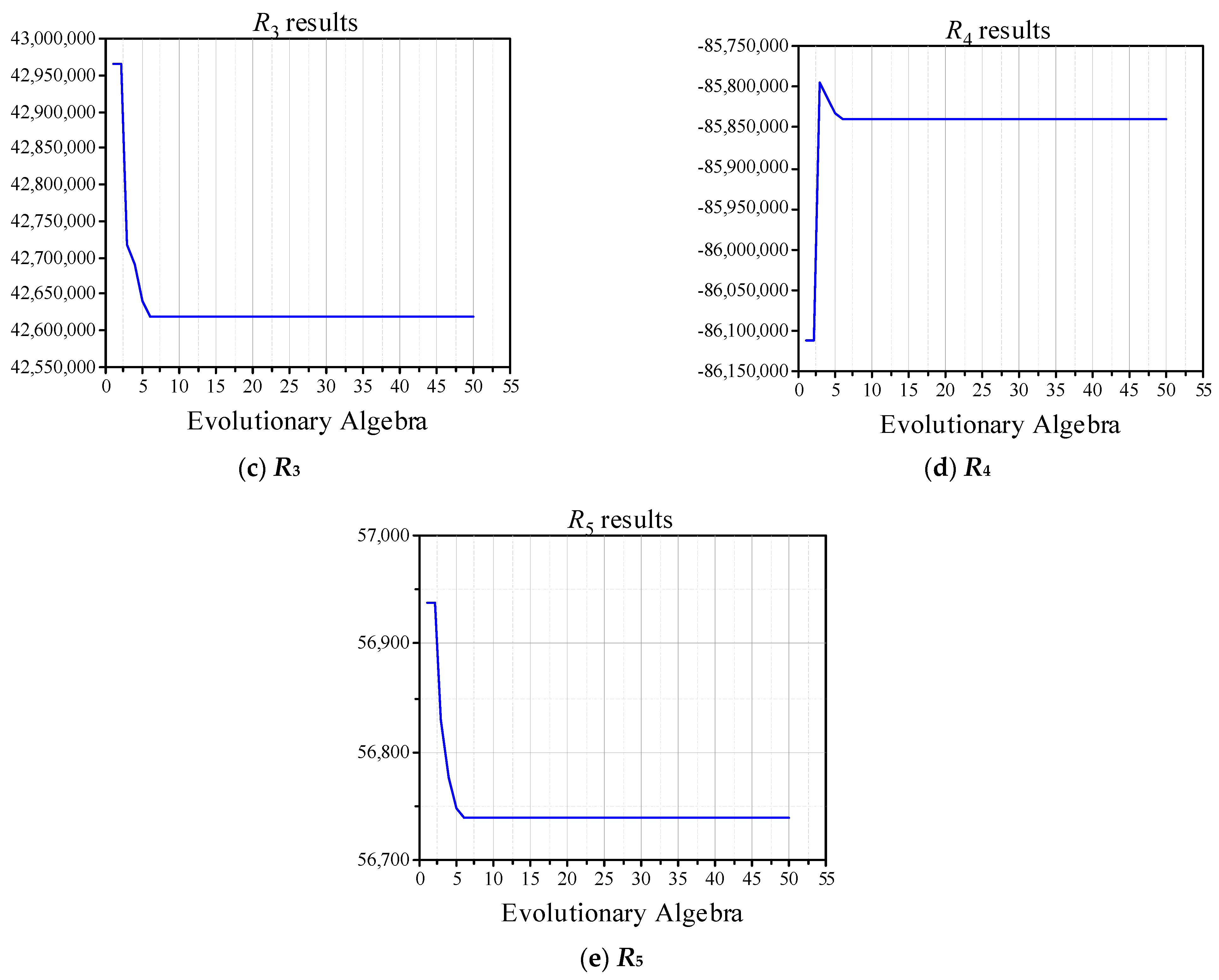
4.3. Pareto Solutions

In practical applications, multi-objective intelligent optimization algorithms are often used to solve the constrained optimization problems of multi-objective functions. Commonly used multi-objective algorithms include multi-objective genetic algorithms, multi-objective simulated annealing algorithms, and multi-objective PSO algorithms. These three types of algorithms are based on different simulation and evolution strategies and transform multi-objective optimization problems into a series of single-objective optimization problems. The goal of the algorithm is to find the optimal solution of the objective function within an appropriate search space while considering the constraints. This process can be achieved by iteratively adjusting the parameters to obtain numerical approximations of the extreme values.
PSO is an efficient parallel search algorithm that can find not only the optimal solution of a problem but also several good suboptimal solutions, thus providing multiple meaningful solutions for practical engineering problems. Based on this, a multi-objective PSO algorithm was used to optimize the response surface fitting equation system. According to the actual engineering needs, under a constant load, the importance ranking of design response objectives is as follows: upper structure engineering quantity > mid-span vertical deflection > axial force of the compressive chord air tube at the pier top > axial force of the stiffening truss > longitudinal internal force of the bridge deck bottom plate.
The PSO program was written using MATLAB, and the operation process of the PSO algorithm is displayed in Figure 10.
The specific optimization process is as follows.
(1)
Initialize the particle population size as N = 500, the particle dimension as D = 4, the maximum number of iterations as T = 50, and the learning factors as c1 = c2 = 1.49445. Determine the particle position range by Table 1; the maximum particle velocity is vmax = 1 and the minimum particle velocity is vmin = −1.
(2)
Initialize the population with random particle positions x and velocities v within the specified range, the individual best position p and the best value pbest for each particle, and the global best position g and best value gbest for the entire swarm.
(3)
Calculate the fitness function based on the response surface equation system and supplement the fitness weighting matrix to regulate the importance ranking of multi-objective parameter optimization.
(4)
Calculate the individual best value for each particle to screen out the global best value for the entire swarm.
(5)
Update all particle positions x and velocity values v, handle the boundary conditions, and update the individual best position p and best value pbest, as well as the global best position g and best value gbest for the entire swarm.
(6)
Check if the termination condition is met (i.e., reaching the maximum number of iterations); if so, terminate the search process and output the global optimization value; otherwise, continue with iteration optimization.
The fitness evolution curve after optimization is shown in Figure 11.
From Figure 11, it can be seen that the fitness function quickly converges after 13 iterations. At this point, the optimized results of R1-R5 are, respectively, −777.910, 65,492,000, 42,620,000, 85,839,000, and 56,738.600. The function optimization curves are shown in Figure 12.

4.4. Optimization Result Certification

To verify the accuracy of the optimization results, an additional multi-objective optimization program based on NSGA-II (non-dominated sorting genetic algorithm II) was written using MATLAB. This program was used to compare the optimization results with those obtained from WPSO. NSGA-II is a multi-objective optimization algorithm based on the genetic algorithm and simulates the process of natural selection and evolution to find optimal solutions. The flowchart of the NSGA-II algorithm is displayed in Figure 13.
The same optimization function and constraints were set for both algorithms. The primary goal was minimizing the engineering quantity of the upper structure, and the secondary goals were minimizing the mid-span vertical deflection and axial internal force of the empty tube of the web bar under compression at the pier top, while ensuring the safety of the bridge structure. Five sets of better optimization results were then selected from the outcomes and the best data were compared. The optimization results obtained using NSGA-II are presented in Table 4, while the optimization results obtained using WPSO are shown in Table 5.
From Table 4, it can be seen that Solutions 2 and 4 are the two methods that achieved the minimum engineering quantity for the upper structure. Although Solution 2 yielded a slightly better optimization result for the mid-span vertical deflection, Solution 4 had a larger optimization magnitude for the upper structure quantity. Moreover, Solution 2 resulted in the negative optimization of the axial internal forces of the stiffened string and the empty tube of the web bar under compression at the pier top, which would affect the structural load-bearing capacity. Therefore, Solution 4 was selected as the final optimization result for NSGA-II.
From Table 5, it can be observed that the optimization magnitudes of each solution of WPSO were quite similar, and there were no extreme cases, as in Solution 2 of NSGA-II. Among them, Solution 3 had the largest optimization magnitude for the engineering quantity of the upper structure, while other optimization indicators did not display significant differences compared to other solutions. Therefore, Solution 3 was selected as the final optimization result for WPSO. The comparison of the final optimization coefficient for both methods is shown in Figure 14.
Figure 14 compares the optimization results of the final solutions of the two optimization algorithms. Compared to the NSGA-II optimization results, WPSO yielded a 6.29% smaller mid-span vertical deflection, a 1.42% larger axial internal force of the stiffened string, a 1.5% smaller longitudinal internal force of the bridge deck bottom plate, a 0.21% smaller axial internal force of the empty tube of the web bar under compression at the pier top, and a 0.45% larger upper structure quantity.
In comprehensive consideration of the optimization targets, it is preferred to minimize the upper structure quantity while ensuring safety, followed by minimizing the mid-span vertical deflection and the axial internal force of the empty tube of the web bar under compression at the pier top. Although the WPSO optimization solution displayed a slight disadvantage in the optimization coefficients of the upper structure quantity and the axial internal force of the stiffened string compared to the NSGA-II solution, it achieved an ad-vantage in the optimization coefficients of the mid-span vertical deflection, the longitudinal internal force of the bridge deck bottom plate, and the axial internal force of the empty tube of the web bar under compression at the pier top. Among them, the optimization co-efficient of the mid-span vertical deflection was almost three times that of the NSGA-II solution. Therefore, considering all the factors, the WPSO optimization solution was chosen as the final optimization solution for the bridge.
After optimization, the vertical deflection at the midpoint of the span can be reduced by 11.09%, the axial internal force of the stiffening member can be reduced by 3.92%, the axial internal force of the bottom plate of the bridge panel can be reduced by 7.56%, and the axial internal force of the compressed web member at the pier top can be reduced by 4.45%. Moreover, the engineering quantity of the upper structure can be reduced by 8.38%. The optimization coefficients are shown in Figure 15.
To compare the lightweight equation with the traditional ABAQUS calculation results and to facilitate visualization, a comparison chart of the calculation data was drawn based on a deflection of 1 mm, an internal force of 105 MPa, and an engineering quantity of 102 t, as presented in Figure 16. After comparison, the maximum deviation between the lightweight calculation using the RSM and the ABAQUS modeling results was found to be 1.43%, which meets the precision requirements while reducing the computational modeling workload.

5. Conclusions

In this study, the elastic modulus of the steel, the thickness of the bridge deck panel, the height of the vertical stiffening rods, and the relative distance between double-layer main beams were selected as the structural parameters to be optimized based on the characteristics of bridge structures supported by engineering. Via the static analysis of the initial FE model in ABAQUS, the mid-span vertical deflection, the axial internal force of the stiffening chord, the longitudinal internal force of the bottom plate of the bridge deck panel, the axial internal force of the compressed chord of the pier top truss, and the quantity of upper structure engineering were selected as the objective functions. A lightweight calculation equation based on the RSM was established for the optimization of the design parameters, and the following conclusions were drawn.
(1)
A lightweight calculation equation based on the FE model of the engineering structure supported by the RSM was established. Via significance analysis, it was found that the use of a simplified incomplete quadratic polynomial as the response surface equation can accurately fit the numerical relationships between the optimized parameters and the target response function to be corrected. The fitting accuracy was found to be high, which greatly reduces the workload of structural modeling in the optimization design and ensures the accuracy and reliability of the optimization.
(2)
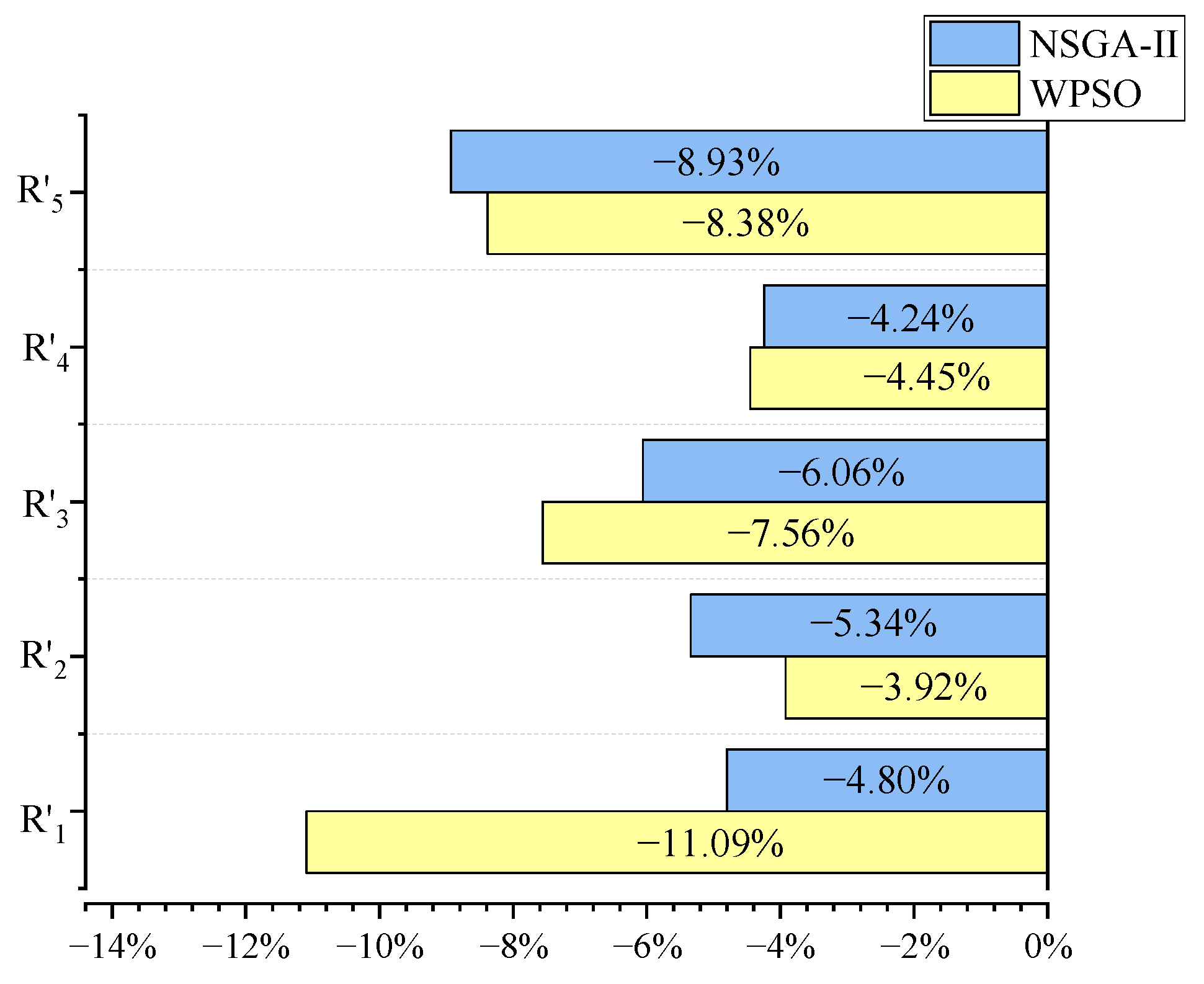
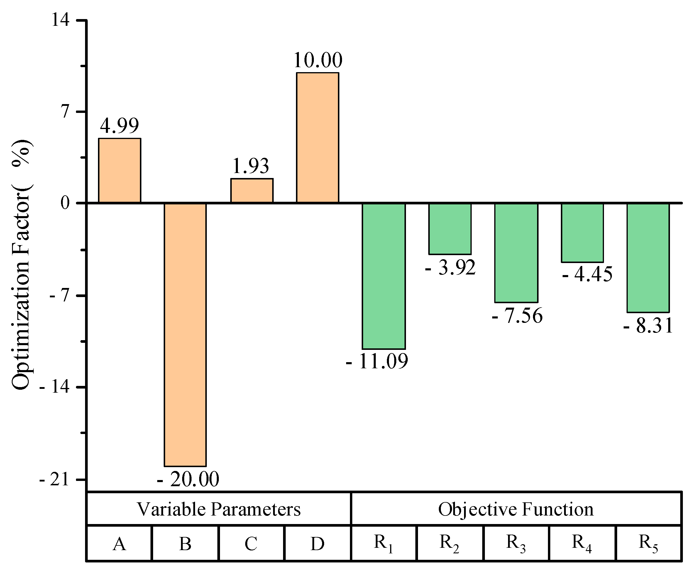
Based on the lightweight equation established using the RSM, two optimization methods, namely, WPSO and NSGA-II, were used to minimize the quantity of upper structure engineering as the primary control objective and to minimize the mid-span vertical deflection and the axial compression force in the hollow pier top tie rod as the secondary control objectives. After comparing the optimization results, WPSO was chosen as the final optimization scheme. After optimizing the design parameters, the mid-span vertical deflection under constant load, the axial internal force of the stiffening chord, the longitudinal internal force of the bottom plate of the bridge deck panel, and the axial internal force of the compressed chord of the pier top truss were reduced by 3% to 11% as compared with the original design. Furthermore, the quantity of upper structure engineering was reduced by 8.38%, which improved the structural performance while reducing the engineering cost.
(3)
In the design stage, bridge structures usually require the manual adjustment of a large number of design parameters to achieve the control of the structural performance, material usage, and engineering cost. The process of establishing complex FE models and adjusting parameter combinations is time-consuming and difficult to control and involves many iterations. This article proposed a method that can achieve the accurate optimization reasoning of certain control indicators of bridge structures via mathematical optimization using lightweight response surface equations. Moreover, when bridge structures enter the service period, this method can still be used to simulate the actual parameters of the bridge structure under current conditions by using health monitoring data. Thus, the precise simulation of the entire life cycle of the bridge structure can be achieved. Therefore, this method is suitable not only for the optimization of structural parameters in the bridge design stage but also for the simulation of the structural health status of bridge structures in the operation stage.

Author Contributions

Conceptualization, L.W. and Y.M.; methodology, L.W.; software, L.W. and R.X.; validation, R.X., X.G. and Y.M.; formal analysis, L.W.; investigation, R.X.; resources, X.G.; data curation, R.X. and Y.M.; writing—original draft preparation, R.X., X.G. and L.W.; writing—review and editing, R.X. and L.W.; visualization, Y.M.; supervision, L.W.; project administration, R.X. and X.G.; funding acquisition, L.W. All authors have read and agreed to the published version of the manuscript.

Funding

This research was funded by the National Key Research and Development Program of China (Grant No. 2021YFB1600305), the Natural Science Basic Research Program of Shaanxi (Program No. 2022JC-23), and the Innovation Capability Support Program of Shaanxi (Program No. 2023-CX-TD-38).

Institutional Review Board Statement

Not applicable.

Informed Consent Statement

Not applicable.

Data Availability Statement

The data that support the findings of this study are available from the corresponding author upon reasonable request.

Conflicts of Interest

The authors declared no conflict of interest.

Nomenclature

RSMResponse surface method
WPSOWeighted particle swarm optimization
FEFinite element
PSOParticle swarm optimization
CCDCentral composite design
MPCMultipoint constraint
C.V.Coefficient of variation
NSGA-IINon-dominated sorting genetic algorithm II

References

  1. Zheng, K.; Feng, X.; Heng, J.; Zhang, Y.; Zhu, J.; Lei, M.; Wang, Y.; Hu, B.; Xiong, Z.; Tang, J.; et al. State-of-the-art review of steel bridges in 2020. J. Civ. Environ. Eng. 2021, 43, 53–69. [Google Scholar]
  2. Dai, J.; Qin, F.; Di, J.; Chen, Y. Review on Cable Force Optimization Method for Cable-stayed Bridge in Completed Bridge State. China J. Highw. Transp. 2019, 32, 17–37. [Google Scholar]
  3. Ye, D.; Xu, Z.; Liu, Y.Q. Solution to the problem of bridge structure damage identification by a response surface method and an imperialist competitive algorithm. Sci. Rep. 2022, 12, 13. [Google Scholar] [CrossRef]
  4. Fang, S.J. Damage detection of long-span bridge structures based on response surface model. Therm. Sci. 2020, 24, 1497–1504. [Google Scholar] [CrossRef]
  5. Li, F.; Liu, Y.K.; Yang, J. Durability assessment method of hollow thin-walled bridge piers under rockfall impact based on damage response surface. Sustainability 2022, 19, 12196. [Google Scholar] [CrossRef]
  6. Miao, C.Q.; Zhuang, M.L.; Dong, B. Stress corrosion of bridge cable wire by the response surface method. Strength Mater. 2019, 51, 646–652. [Google Scholar] [CrossRef]
  7. Hu, S.; Chen, B.; Song, G.; Wang, L. Resilience-based seismic design optimization of highway RC bridges by response surface method and improved non-dominated sorting genetic algorithm. Bull. Earthq. Eng. 2022, 20, 449–476. [Google Scholar] [CrossRef]
  8. Li, H.; Li, L.; Wu, W.; Xu, L. Seismic fragility assessment framework for highway bridges based on an improved uniform design-response surface model methodology. Bull. Earthq. Eng. 2020, 18, 2329–2353. [Google Scholar] [CrossRef]
  9. Chen, L.; Huang, C.; Gu, Y. Seismic vulnerability analysis of simply supported highway bridges based on an improved response surface method. Eng. Mech. 2018, 35, 208–218. [Google Scholar]
  10. Ma, Y.; Liu, Y.; Liu, J. multi-scale finite element model updating of CFST composite truss bridge based on response surface method. China J. Highw. Transp. 2019, 32, 51–61. [Google Scholar]
  11. Ji, W.; Shao, T.Y. Finite element model updating for improved box girder bridges with corrugated steel webs using the response surface method and fmincon algorithm. Ksce J. Civ. Eng. 2021, 25, 586–602. [Google Scholar] [CrossRef]
  12. Zhang, L.; Wang, B.; Wang, B.; Chen, K.; Lü, J. A method for modifying dynamic model of cable-stayed bridge based on response surface method. J. Highw. Transp. Res. Dev. 2022, 39, 46–52, 61. [Google Scholar]
  13. Li, Y.; Liu, X.; Chen, Z.; Zhang, H. Updating of cable-stayed bridge model based on cable force response surface method. J. China Railw. Soc. 2021, 43, 168–174. [Google Scholar]
  14. Sun, Y. Research on Computational Model Modification of Steel-Concrete Composite Beam Self-Anchored Suspension Bridge Based on Response Surface Method. Master’s Thesis, Central South University, Changsha, China, 2020. [Google Scholar]
  15. Zhang, Q. Study on preparation and mechanical properties of green bridge concrete building materials: Based on response surface method. Fresenius Environ. Bull. 2021, 30, 5816–5825. [Google Scholar]
  16. Lehky, D.; Somodikova, M.; Lipowczan, M.; Novak, D. Inverse response surface method for prestressed concrete bridge design. In Proceedings of the 10th International Conference on Bridge Maintenance, Safety and Management (IABMAS), Electr Network, Sapporo, Japan, 11–18 April 2021; CRC Press-Balkema: Boca Raton, FL, USA, 2021. APR 11-18. [Google Scholar]
  17. Zhan, Y.; Hou, Z.; Shao, J.; Zhang, Y.; Sun, Y. Cable force optimization of irregular cable-stayed bridge based on response surface method and particle swarm optimization algorithm. Bridge Constr. 2022, 52, 16–23. [Google Scholar]
  18. Wang, D.; Zhou, W.; Li, M. Research on weight asymmetry alignment correction of main girder of long-span concrete cable-stayed bridge based on response surface method. Highw. Automot. Appl. 2022, 2, 94–96. [Google Scholar]
  19. Bruno, D.; Lonetti, P.; Pascuzzo, A. An optimization model for the design of network arch bridges. Comput. Struct. 2016, 170, 13–25. [Google Scholar] [CrossRef]
  20. Lonetti, P.; Pascuzzo, A. Design analysis of the optimum configuration of self-anchored cable-stayed suspension bridges. Struct. Eng. Mech. 2014, 51, 847–866. [Google Scholar] [CrossRef]
  21. Wu, Z.; Liu, J.; Zou, D.; Wang, X.; Shi, J. Status quo and development trend of light-weight, high-strength, and durable structural materials applied in marine bridge engineering. Strateg. Study CAE 2019, 21, 31–40. [Google Scholar] [CrossRef]
  22. Peng, Z. Research on the Strengthening and Toughening Mechanisms of Ti Microalloyed Hot-Rolled High-Strength Steel Plates. Master’s Thesis, South China University of Technology, Guangzhou, China, 2016. [Google Scholar]
  23. Liu, Y. Research on the Influence of Size Parameter and Section Form on the Stress of Orthotropic Steel Deck Slab. Master’s Thesis, Lanzhou Jiaotong University, Lanzhou, China, 2018. [Google Scholar]
  24. Su, J.; Wang, F. Brief introduction to design of Zengjiayan Jialing river bridge of Chongqing. Technol. Highw. Transp. 2016, 32, 38–42. [Google Scholar]
  25. Mei, X.; Xu, W.; Duan, X.; Chen, X. Overall design of Pingtan strait combined bridges. Railw. Stand. Des. 2020, 64, 18–23. [Google Scholar]
  26. Yang, Z.; Wang, L.; Wang, J.; Sun, X.; Liang, L. Structural design of main bridge of Niutianyang bridge. Bridge Constr. 2021, 51, 1–8. [Google Scholar]
Figure 1. The flowchart of the capacity design process based on WPSO-SRM.
Applsci 13 11033 g001
Figure 2. The front elevation of the truss bridge (unit: m).
Applsci 13 11033 g002
Figure 3. The main beam section layout (unit: mm). (a) The layout of the main section on the pier top. (b) The layout of the standard main section.
Applsci 13 11033 g003
Figure 4. The multi-scale FE model of the tested bridge.
Applsci 13 11033 g004
Figure 5. The verification of the calculation accuracy. (a) The maximum axial force of the upper chord under the design load. (b) The maximum axial force of the lower chord under the design load. (c) The maximum axial force of the web under the design load. (d) The maximum axial force of the upper stiffened chord under the design load. (e) The maximum axial force of the stiffened vertical bar under the design load.
Applsci 13 11033 g005aApplsci 13 11033 g005b
Figure 6. The design test operating conditions.
Applsci 13 11033 g006
Figure 7. The fitting response surface.
Applsci 13 11033 g007aApplsci 13 11033 g007b
Figure 8. The respective levels of significance. (a) The significance of single factors. (b) The two-way interaction significance. (c) The significance of quadratic coupling terms.
Applsci 13 11033 g008
Figure 9. The comparison of the fitting accuracy.
Applsci 13 11033 g009
Figure 10. The operation process of the PSO algorithm.
Applsci 13 11033 g010
Figure 11. The fitness evolution diagram.
Applsci 13 11033 g011
Figure 12. The optimization curves.
Applsci 13 11033 g012aApplsci 13 11033 g012b
Figure 13. The flowchart of the NSGA-II algorithm.
Applsci 13 11033 g013
Figure 14. The comparison of the optimization coefficients.
Applsci 13 11033 g014
Figure 15. The comparison of the objective function correction results.
Applsci 13 11033 g015
Figure 16. The comparison of the optimization of the computation accuracy.
Applsci 13 11033 g016
Table 1. The parameters to be optimized.
LabelParameterRange of Correction (%)Level
LowInitialHigh
ASteel elastic modulus (MPa)±5195,700206,000216,300
BBridge deck thickness (mm)±2012.81619.2
CMaximum length of vertical stiffening rods (mm)±1028,80032,00035,200
DRelative distance between double-layer main beams (mm)±1010,80012,00013,200
Table 2. The settings of the objective functions.
LabelObjective Function
R 1 Mid-span vertical deflection
R 2 Axial internal force of the stiffened string
R 3 Longitudinal internal force of the bridge deck bottom plate
R 4 Axial internal force of the empty tube of the web bar under compression at the pier top
R 5 Superstructure works
Table 3. The computational probability evaluation.
Experimental Design ElementsStandard DeviationVariance Inflation FactorDesign Assessment Probability Calculation
0.5 Standard Deviation1.0 Standard Deviation2.0 Standard Deviation
A0.20 1.00 20.9%63.0%99.5%
B0.20 1.00 20.9%63.0%99.5%
C0.20 1.00 20.9%63.0%99.5%
D0.20 1.00 20.9%63.0%99.5%
AB0.25 1.00 15.5%46.5%96.2%
AC0.25 1.00 15.5%46.5%96.2%
AD0.25 1.00 15.5%46.5%96.2%
BC0.25 1.00 15.5%46.5%96.2%
BD0.25 1.00 15.5%46.5%96.2%
CD0.25 1.00 15.5%46.5%96.2%
A20.19 1.05 68.7%99.8%99.9%
B20.19 1.05 68.7%99.8%99.9%
C20.19 1.05 68.7%99.8%99.9%
D20.19 1.05 68.7%99.8%99.9%
Table 4. The NSGA-II optimization results.
Optimization GroupOptimization ObjectiveOptimization Coefficient (%)
A
(MPa)
B
(mm)
C
(mm)
D
(mm)
R1′R2′R3′R4′R5′
1216,23712.9434,59913,185−12.97%−2.32%−12.36%−3.38%−7.67%
2216,23712.9534,59912,047−5.80%4.70%−5.38%2.17%−8.57%
3216,23712.9634,99913,185−12.87%−1.82%−13.48%−3.23%−7.57%
4216,27913.0032,61813,200−4.80%−5.34%−6.06%−4.24%−8.93%
5216,23612.9635,13513,185−12.81%−1.63%−13.88%−3.17%−7.55%
Table 5. The WPSO optimization results.
Optimization GroupOptimization ObjectiveOptimization Coefficient (%)
A
(MPa)
B
(mm)
C
(mm)
D
(mm)
R1′R2′R3′R4′R5′
1216,30012.8032,83813,200−11.25%−3.76%−7.90%−4.40%−8.35%
2216,30012.8032,72313,200−11.18%−3.85%−7.72%−4.43%−8.35%
3216,27912.8032,61813,200−11.09%−3.92%−7.56%−4.45%−8.38%
4216,30012.8033,08813,200−11.38%−3.55%−8.30%−4.33%−8.31%
5216,30012.8232,81613,200−11.24%−3.79%−7.86%−4.41%−8.29%
Disclaimer/Publisher’s Note: The statements, opinions and data contained in all publications are solely those of the individual author(s) and contributor(s) and not of MDPI and/or the editor(s). MDPI and/or the editor(s) disclaim responsibility for any injury to people or property resulting from any ideas, methods, instructions or products referred to in the content.

