1. Introduction
With the development of modern automotive industry technology, the research on road slope estimation has received widespread attention. Fully considering the accuracy of slope estimation and the braking force distribution strategy can contribute to the research on an energy recovery strategy of new energy vehicles during braking [
1,
2]. Fuel cell vehicles have been favored by many car manufacturers due to their advantages in environmental protection and energy conservation. Local governments are also continuously refining their policies for fuel cell vehicles. Faced with a promising market, many car companies have also proposed to increase their research and development efforts for fuel cell vehicles [
3,
4,
5]. In addition, the Brake-By-Wire (BBW) system in the field of braking systems has received much attention in recent years [
6], which is also the research content of this article. Using BBW to coordinate the distribution of the braking force can significantly improve the energy recovery efficiency and braking safety of vehicles.
In recent years, researchers, both domestically and internationally, have conducted extensive studies on brake energy recovery strategies. He et al. [
7] designed a control strategy based on braking safety stability and high braking recovery to improve braking energy recovery efficiency while meeting vehicle comfort. With the goal of minimizing energy recovery losses, they designed a regenerative braking control strategy for driving motors, which increased energy recovery efficiency by 3.35%. Xu et al. [
8] proposed a fuzzy control strategy to allocate front and rear wheel braking forces, so that the braking force meets the requirements of the Economic Commission for Europe (ECE) regulations, and a battery temperature factor is designed to correct the calculated regenerative braking force. Kumar, C.N. et al. [
9] proposed a new synergistic control of regenerative and friction braking together in hybrid EVs, which makes the braking force distribution curves of the front and rear wheels close to the ideal distribution curve and facilitates stable braking.CH et al. [
10] proposed a pulse width module (PWM) to control the regenerative braking cycle frequency and regenerative braking control strategy. Improve the efficiency of regenerative braking recovery.
The study of slope is crucial for the development of braking performance, and the lack of slope recognition information may lead to insufficient distribution of the braking force or instability in the reduction process. For example, when a vehicle is uphill, it requires a large amount of power to ensure its speed and performance; when a vehicle brakes downhill, the required power is usually zero, and the driver can predict the slope information to brake reasonably, thereby protecting brake pads and other components to avoid danger such as brake failure [
11,
12].
Mahyuddin et al. [
13] proposed a new observer scheme that utilizes sliding membrane control to estimate road slope, which is inaccurate and has significant errors. Mclntyre et al. [
14] proposed a two-stage estimation strategy for estimating road slope values, but this method requires the use of a single estimator for estimating variable slope roads, which increases the difficulty and complexity of the calculation. Holm et al. [
15] proposed the method of an extended Kalman filter (EKF) to estimate road slope, but it requires a large amount of data input, making the calculation complex.
Li et al. [
16] proposed a two-layer adaptive estimator to estimate road slope values, which does not require additional sensors but still requires a large amount of computation. This method combines quality and slope values, resulting in mutual influence between the two results, and in poor estimation accuracy. Kim et al. [
17] proposed a recursive least squares method to estimate slope values, but this algorithm only considers sensors in vehicles and has certain limitations, so it cannot be widely promoted. Shen et al. [
18] used Bayesian methods to solve the coupling problem of quality and slope, but the computational complexity was large and the algorithm was too complex. In the aforementioned studies, there are numerous computational and algorithmic complexity issues.
In fact, the slope of the road on which the vehicle is driving is always changing, including factors such as noise, making it difficult to develop an optimal braking control strategy [
19]. Considering the crucial impact of braking force distribution on braking energy recovery, this paper uses an optimized adaptive filtering algorithm to estimate the vehicle’s driving slope, enabling the vehicle to obtain more accurate road slope information. Then, based on the slope information, a braking control strategy is specified to distribute regenerative braking force while meeting ECE regulations, thereby improving energy recovery efficiency.
The structural framework of the remaining parts of this article is as follows: In the
Section 2, a vehicle longitudinal dynamics model is established, and the vehicle speed and acceleration are obtained from the sensors. Therefore, only longitudinal acceleration and velocity sensors need to be added, and data such as wheel torque are obtained from the Controller Area Network (CAN) bus to establish a prediction process and observation equation. In the
Section 3, we address the shortcomings of Sage–Husa adaptive filtering and combine it with the corrected fading factor and adaptive factor of the strong tracking Kalman filter to update the original Kalman gain and posterior error covariance matrix, constructing a new adaptive optimization algorithm. The
Section 4 combines the estimated slope value with the optimized braking force distribution strategy to obtain a new braking force distribution coefficient and complete the braking force distribution. The
Section 5 conducts experimental simulation analysis, compares the optimized adaptive filtering algorithm with the original adaptive filtering algorithm, and conducts vehicle braking energy recovery simulation experiments to draw conclusions. The
Section 6 summarizes the whole paper and makes a prospect. The technical roadmap of this article is shown in
Figure 1.
2. The Model
2.1. The Vehicle Longitudinal Dynamics Model
In this study, only the longitudinal dynamic motion of fuel cell commercial vehicles was considered. The force acting on the vehicle on a slope is shown in
Figure 2. When driving on a slope, the vehicle is affected by driving force, slope resistance, air resistance, and rolling resistance. Therefore, the longitudinal dynamic equation of the vehicle is:
where
,
,
,
and
are the driving force, rolling friction force, gradient resistance, aerodynamic resistance and uphill driving force, respectively.
Among them, the expression for the slope resistance
is:
In the equation, represents the gravitational acceleration, and represents the angle of the slope.
The expression for the driving force
is:
In the equation, is the actual torque input from the engine to the transmission; is the transmission ratio of the gearbox; is the main reducer transmission ration; is the mechanical efficiency of the transmission; is the rolling radius.
The expression for the air resistance
is:
In the equation, is the air density coefficient, A is the vehicle frontal area, is the air density, is the speed of the vehicle.
The expression for the rolling resistance
is:
In the equation, m is the mass of the vehicle.
The nonlinear equation of the vehicle’s longitudinal dynamics is expressed as
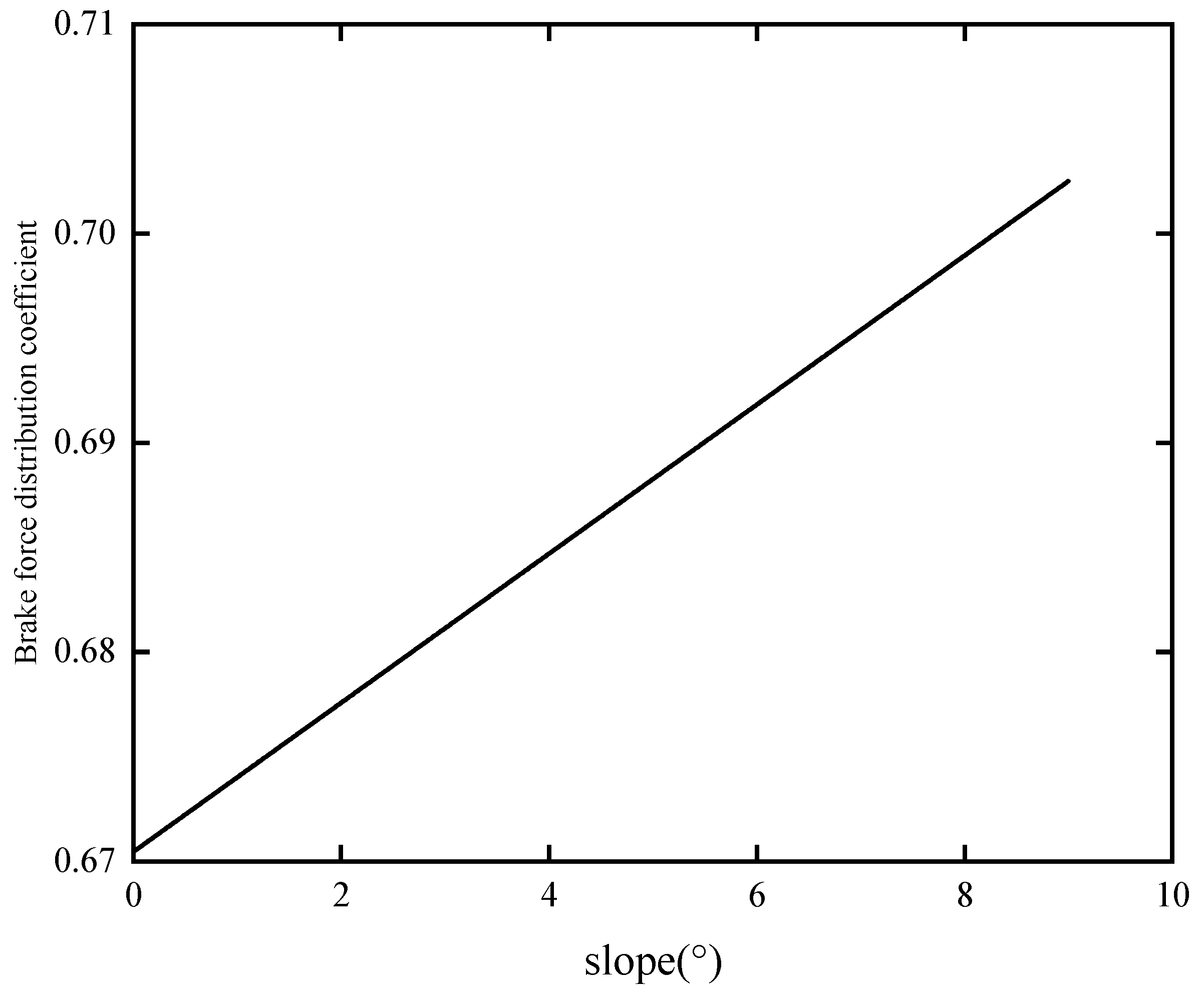
Based on practical analysis, in highway design standards, the longitudinal slope of the road is not greater than 9%, and the corresponding angle is within 5°. Therefore, in cases of smaller angles, it can be considered that the tangent and sine values of the slope angle are equal. So, the Equation (6) can be changed to:
The windward area A of the fuel cell commercial vehicle used in this article is 6.6454, and the wind resistance coefficient is generally taken as an empirical value. In this article, is 0.563.
2.2. Establishment of the Prediction Equation and the State Equation
In this article, appropriate state variables should be selected for observation, namely driving speed
v and road slope
i, because these two parameters are easy to read. At this time, the state variable
x can be expressed as:
In general, the change in road slope is slow, and the driving speed of commercial vehicles is relatively low. Therefore, the differential equation for speed and slope can be obtained as:
The estimation of slope value using kinematic methods is based on the kinematic equation, where the car’s acceleration can be obtained through an onboard accelerometer. From the relationship between velocity and acceleration, along with the vehicle’s longitudinal dynamics equation, we can derive the system’s state equation:
In the formula, and represent the result value of the previous time step, that is, the value at time k without Kalman filtering, and q represents the noise vector of the prediction equation.
During actual driving, the vehicle speed is easily measurable, so if the vehicle speed
v is taken as the observation value, the observation equation can be expressed as:
In the above equation, H = , velocity and slope are set as observed values. However, there may be some noise effects in the experiment that are unmeasurable, so the prediction equation error cannot be ignored. Therefore, in this paper, the noise is considered, and the r represents the measured noise vector.
3. The Adaptive Kalman Filter
3.1. Kalman Filtering
As shown in
Figure 3, the process of the Kalman filter can be categorized into two types: prediction and update. It is an optimal state estimation algorithm. The variables in the Kalman filter include state variables and observation variables. The Kalman filter algorithm aims to continuously approximate the true data by merging the state variables and observation variables, obtaining the value closest to the true data. This value is then used as the variable for the next state, and the process is iteratively repeated by merging it with the observation variables at the next moment.
Firstly, we substitute the optimal estimate value at time k − 1 into the prediction equation, which allows us to calculate the a priori estimate value at time k. Then, we compare the a priori estimate value at time k with the measurement value . By using the Kalman gain, we update both of these values to obtain the optimal estimate value at time k. This process is repeated iteratively until the estimate value becomes closer to the true value.
The Kalman filtering algorithm is mainly expressed by five formulas:
- 1.
Prediction equation
The covariance expression of the prior error is
In the formula, P is the prior error covariance, used to measure the uncertainty in the predicted state, is the error between the process error and the estimated value, and Q is the covariance matrix of the predicted noise.
- 2.
Update equation
The updated Kalman gain can be represented as:
In the formula, is the Kalman gain, which is the difference between the predicted value and the true value. R is the covariance of the observed values, representing the uncertainty of the state.
Best estimate value
update equation for k is:
In the formula, .
Posteriori error covariance
is:
In the formula, I is identity matrix, and the order is equal to the order of the state variable.
3.2. The Sage–Husa Adaptive Kalman Filter Principle
This algorithm is a derivative algorithm of Kalman filtering, which can target uncertain
Q-
matrices and
R-
matrices, namely the covariance matrix corresponding to process noise and measurement noise. This adaptive algorithm is mainly based on the minimum mean square error, and then uses observation data to recursively solve, while using a time-varying noise estimator to estimate and correct the statistical characteristic parameters of system noise and measurement noise in real time, achieving the goal of reducing model errors, suppressing filtering divergence, and improving accuracy [
20]. Adaptive Kalman filtering is an extension of the standard Kalman filter that updates the parameters
and
based on the estimation error and the characteristics of the system being modeled. The specific coefficients are expressed as follows:
Weighted coefficient
can be expressed as:
The parameter , which takes values between 0.95 and 0.99, is primarily used to enhance the influence of the previous time step’s data on the current time step’s result and update the noise in adaptive filtering.
The specific update steps are as follows:
Although time-varying noise statistical estimators can update Q and R, improving estimation accuracy, the uncertainty in dynamic models can affect the filtering process.
3.3. The Improved Adaptive Kalman Filter
In response to the shortcomings of Sage–Husa adaptive filtering, this paper proposes an optimized adaptive filtering algorithm, which improves the traditional algorithm and combines it with strong tracking filtering algorithm. In order to suppress disturbances in the dynamic model and abnormal observations, and improve the accuracy of estimation, the algorithm improvement steps are as follows.
3.4. Construction of Strong Tracking Filter Factors
In practice, traditional adaptive filtering is prone to noise interference, leading to a decrease in measurement accuracy. In order to improve the accuracy of adaptive filtering, an adaptive fading factor can be added to achieve and correct the prediction error covariance matrix. Among them,
can represent the true estimation error, and the variance matrix
can represent the theoretical prediction error, which is expressed as:
The judgment criteria are:
The variable
is an adjustable coefficient. When
≥ 1,
can be expressed as:
In the formula, when
is an adjustable coefficient, and
≥ 1, it can be calculated using the following equation:
In the formula,
represents the covariance matrix of the residual vector,
β is the suppression factor, and tr(·) denotes the trace of a matrix.
can be expressed as:
where
is the forgetting factor and
represents the sliding window, it can be expressed as:
where
is the sliding window size type.
Constructing an Adaptive Factor Three-Stage Equation
To obtain the optimal estimation from adaptive Kalman filtering, it is necessary to calculate the corresponding covariance matrix and adaptive factor. Yang et al. [
21] proposed four error discrimination statistics for constructing the adaptive factor
, including the state inconsistency statistic, the prediction residual statistic, the variance component ratio statistic, and the velocity inconsistency statistic. In this study, to mitigate the impact of unreliable observation information on
, the state inconsistency statistic is selected and a three-stage construction is employed for the adaptive factor. It can be expressed as:
In the formula, 1 ≤
≤ 1.5, 3 ≤
≤ 4.5,
is the statistical measure of inconsistent values in state statistics, expressed as:
Therefore, the filtering gain
and the posterior error covariance
can be reexpressed as:
The optimized algorithm in this study combines the modified decay factor and adaptive factor from the strong tracking Kalman filter, updating the original Kalman gain and posterior error covariance matrix. This eliminates filter divergence and increases the accuracy and stability of the algorithm estimation, compared to the previous adaptive algorithm. The algorithm process is shown in
Figure 4 5. Experimental Simulation and Conclusions
5.1. Construction of the Experimental Simulation Platform
A comprehensive vehicle model of a fuel cell commercial vehicle was established on the AVL_CRUISE2019 vehicle simulation platform to conduct vehicle dynamic simulations. The Matlab2021/Simulink platform was utilized to construct an exquisite fuel cell power tracking system, which effectively regulates the output power of both fuel cells and power cells. Simulation output data were used as a substitute for actual output data. For example, motor torque data and vehicle speed data were transmitted to the Simulink model through a connection interface. A robust adaptive filtering model known as strong tracking adaptive filter was implemented in Simulink. Additionally, to account for the data acquisition errors introduced by the CAN bus, and to reflect the realism of data acquisition, Gaussian white noise was added to the vehicle speed and motor torque in the Matlab environment. The added Gaussian white noise followed a Gaussian distribution.
Figure 8 illustrates the joint simulation process of the software.
Taking a fuel cell commercial vehicle of a certain company as an example for research, the vehicle parameters are shown in
Table 2.
The rolling radius of the tire is selected based on the 8.25R16 tire, taking into account sufficient load-bearing capacity and wear resistance. The rotational mass conversion coefficient of the vehicle is 1.1. The curb weight includes the weight of the vehicle itself, experimental instruments, and personnel.
The power system of fuel cell commercial vehicles in work consists of a power transmission system integrator, power battery control system, power battery, motor control system, and motor.
Figure 9 shows the entire vehicle transmission system.
5.2. Construction of the Electric Power following System
The fuel cell and power cell work together to supply energy for the fuel cell commercial vehicles’ electrical system. Together with the fuel cell, the power cell is a crucial auxiliary energy source in the fuel cell power system, supplying the necessary power for the vehicle during load beginning, acceleration, and climbing. It also recovers some of the brake energy used during vehicle deceleration and braking. Fuel cell vehicles obtain their power mostly from fuel cells, which are devices that directly transform chemical energy into electrical energy. To balance the two types of batteries, the Matlab/Simulink platform was utilized to construct an exquisite power tracking system, which effectively regulates the output power of both fuel cells and power cells. The core idea of the power following system is to maintain the battery working in the optimal range and accurate output power, The power following system includes the following types [
28]:
Firstly, the power of fuel cells and power cells should be evaluated, express as:
Step1: The fuel cell and power batteries are inoperable when the vehicle is not started, expressed as:
Step2: When the vehicle is in braking condition, the State of Charge (SOC) of the power battery is lower than the SOC
max (the highest critical point of power batteries), with the fuel cell output mode off, and the regenerative braking mode activated, expressed as:
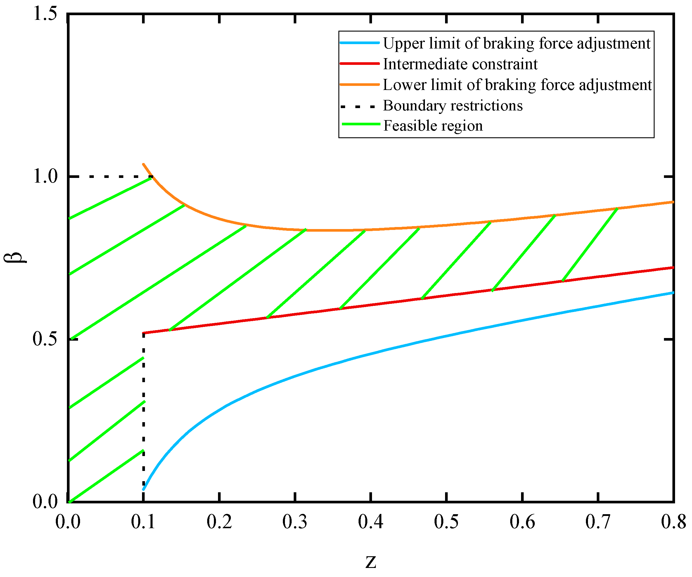
In the formula, is the braking force distribution coefficient and is the vehicle power demand.
Step3: The power cell uses all of its energy when the vehicle is first started since the fuel cell’s immediate power is insufficient. It is decided whether to turn on the fuel cell once the necessary circumstances are met.
Step4: The analysis of the working conditions of the power battery and fuel cell during normal vehicle operation is as follows:
- 1.
The power battery operates independently
When the power demand of the entire vehicle is low and the output power of the power battery is greater than the demand power, and the SOC of the power battery is greater than SOCmax, the fuel cell is closed.
- 2.
Fuel cells work independently
When the fuel cell starts normally and the maximum output power of the power battery cannot meet the normal demand power, and the SOC of the power battery is less than the set expected value, the charging mode is activated to restore the SOC of the power battery to the expected value. The power relationship is as follows:
In the formula, is the set SOC expectation value, and are the maximum and minimum value of SOC for power batteries.
- 3.
Joint output of power cells and fuel cells
When the vehicle is in the acceleration or climbing stage, the output power of the fuel cell is not enough to meet the power demand of the vehicle, and the SOC of the fuel cell is greater than the set expected value. At this time, the output power of the power cell will be controlled to ensure that the fuel cell operates efficiently. The power relationship is as follows:
5.3. Slope Estimation Algorithm Validation
5.3.1. Experimental Plan
In order to verify the effectiveness of the improved adaptive filtering in road slope estimation, this paper conducted vehicle testing and simulation, tested on flat roads and variable slopes, and compared it with the adaptive Kalman filtering to verify the accuracy of the improved algorithm.
The strong tracking filtering algorithm filters the acceleration transmitted by the acceleration sensor, eliminating the noise and error effects during the measurement process.
Figure 10a displays the filtering effect, where the blue portion represents the signal measured from the acceleration sensor, and the red line represents the filtered signal. It can be observed that the strong tracking filter provides a good filtering effect on the measured values.
Figure 10b depicts the variable slope changes in the slope gradient.
5.3.2. Identification Results and Error Analysis
Internationally, road slope classifications mainly include the following categories: normal slope ranging from 0° to 0.5°, slight slope from 0.5° to 2°, gentle slope from 2° to 5°, and moderate slope from 5° to 15°. In the Cruise2019 simulation software, road conditions with gentle slopes and variable slopes were specifically created to verify the accuracy of the strong tracking filtering algorithm. The term “gentle slope” refers to slopes with good road conditions and a gradual change in slope. “Variable slope” refers to slopes with significant changes in slope, characterized by an unstable rate of change.
Figure 11b illustrates the variations in the slope gradient for the variable slope condition.
Figure 11 presents the performance and error slopes of the Strong Tracking Adaptive Filter (STF) and the Adaptive Filter (AF) algorithms for identifying gentle slopes and variable road slopes. The algorithms were applied to both fixed slope road segments and variable slope road segments for identification. In the case of variable slope roads, as shown in
Figure 11a, the fluctuation frequency of the STF algorithm is lower than that of the AF algorithm, indicating that the STF algorithm performs better in slope identification with good tracking performance. From
Figure 11c, it can be observed that the identification error of STF is generally controlled within 1°, while the identification accuracy of AF is significantly lower, with a higher error rate compared to STF. As shown in
Figure 11b, for fixed slopes, the identification curve of STF is closer to the reference slope and exhibits smaller fluctuations compared to AF, although the difference between the two is not substantial. From
Figure 11d, it can be seen that the identification error range of STF is smaller than that of AF. Vahidi suggests that when the slope identification error is within 0.2°, it can be considered as reaching a stable state of slope identification [
29].
Based on the estimated road slope from the vehicle’s travel analysis, the identified road slope information is analyzed in terms of the mean absolute error (MAE) and the root mean square error (RMSE). The analysis results are presented in
Table 3. The calculation formula for the mean absolute error is:
The formula for calculating the root mean square error is:
From
Table 3, it can be observed that in terms of the MAE, during the fixed slope phase, the STF algorithm has a smaller average absolute error compared to the AF algorithm. This holds true during the variable slope phase as well. For the RMSE, the STF algorithm exhibits a smaller root mean square error than the AF algorithm, both during the fixed slope and variable slope phases. In conclusion, the STF algorithm outperforms the AF algorithm in terms of identification accuracy.
5.4. Braking Energy Recovery
This study plans to use the CHTC-HT operating condition and C-WTVC operating condition for simulation validation. The evaluation criteria will be the braking energy recovered by the power battery during vehicle braking. For both of these operating conditions, they will be combined with uphill road slopes of 0° and 5°. To highlight the energy recovery effect during road slope identification and braking force optimization allocation strategies, a comparison will be made with the series brake regeneration strategy during simulation.
5.4.1. Simulation under CHTC-HT Operating Condition
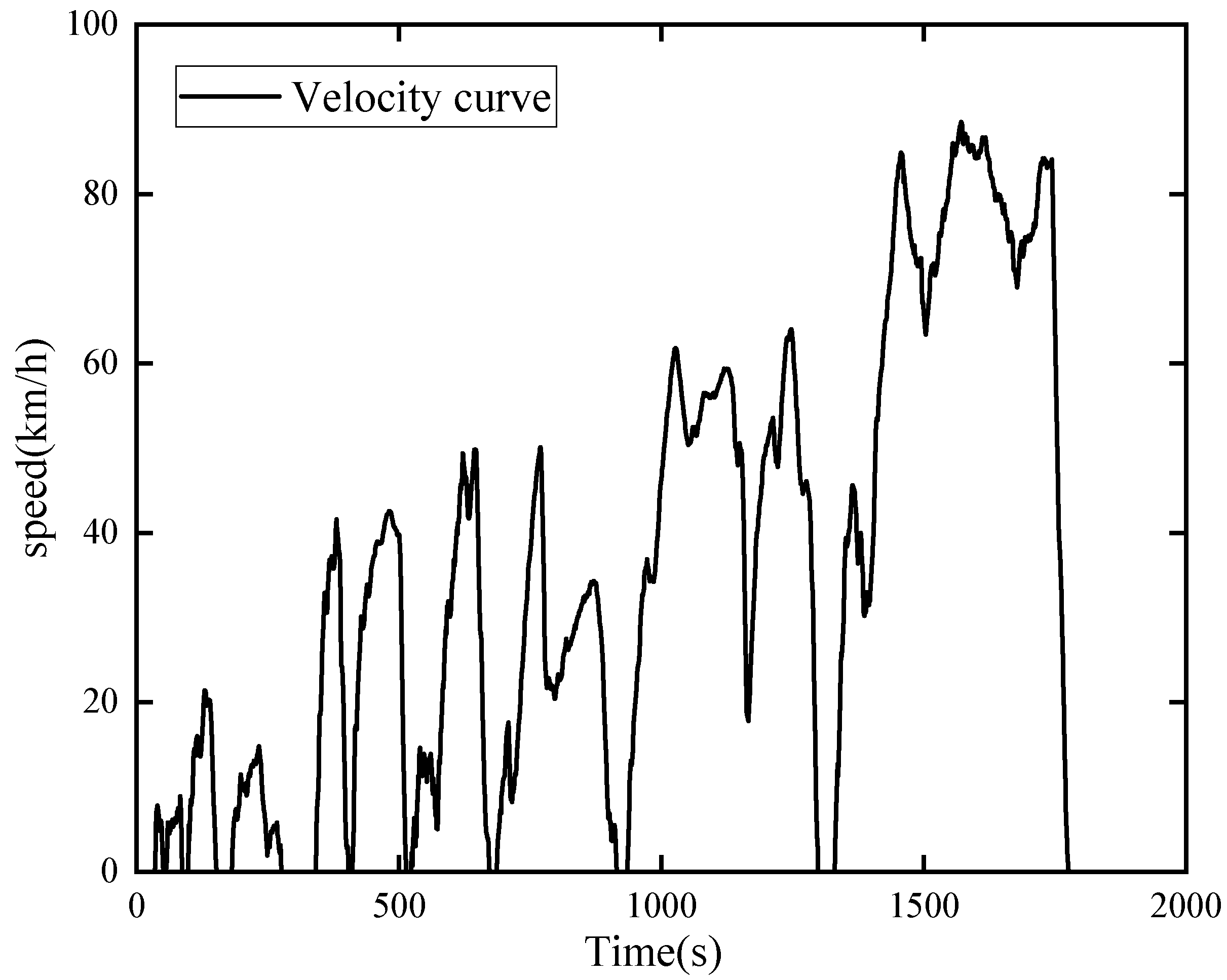
The CHTC-HT operating condition consists of three speed intervals, with a total duration of 1800 s. The urban interval accounts for 19% of the total operating condition duration, the suburban interval accounts for 54.9%, and the highway interval accounts for 26.1%. The average speed throughout the operating condition is 34.7 km/h, with a maximum vehicle speed of 88.5 km/h. The speed profile of the CHTC-HT operating condition is shown in
Figure 12.
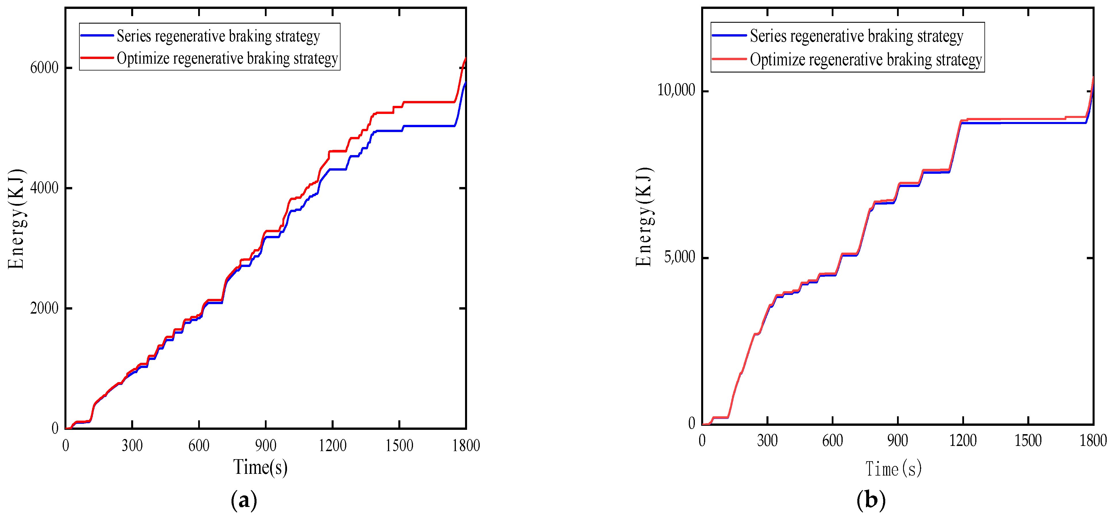
Under the CHTC-HT condition, when the slope angles are 0° and 5°, a comparison was made between the case without slope detection and brake force allocation strategy, and the case with slope detection and brake force optimization strategy. Energy recovered from power batteries is shown in
Figure 13a,b.
From
Figure 13a, it can be observed that when the vehicle travels on a flat road for 1800 s, The energy recovery of power batteries is gradually increasing. At 450 s, the optimized regenerative braking strategy starts to take effect, resulting in the amplitude of energy recovery from power batteries has begun to significantly increase. Since the vehicle is in a low-speed phase, the output power from the fuel cell is stored in the power battery in the form of electrical energy, hence the Energy recovery is on the rise. During the periods from 950 s to 1150 s and 1450 s to 1750 s, the vehicle operates under high-speed conditions, causing the energy recovery of power batteries is showing a significant upward trend. At 1700 s, the vehicle began to slow down until the speed reached 0, and the recovered energy from the power battery rapidly increased. From
Figure 13b, it can be seen that the vehicle operates on a 5° uphill slope condition, resulting in the trend of energy recovery from power batteries is relatively gentle. However, the regenerative braking strategy based on slope estimation still has a significant improvement in recovery capacity compared to the series regenerative braking strategy.
5.4.2. Simulation Verification of C-WTVC Operating Condition
The C-WTVC operating condition is a driving cycle designed based on the Worldwide Transient Vehicle Cycle (WTVC) for heavy-duty commercial vehicles. It consists of three driving conditions: urban cycle (900 s), highway cycle (468 s), and high-speed cycle (432 s). This driving condition includes numerous acceleration and deceleration segments. The speed statistics of the driving cycle are shown in
Table 4, and the speed profile of the driving condition is illustrated in
Figure 14.
Under the C-WTVC condition, when the slope angles are 0° and 5°, a comparison was made between the case without slope detection and brake force allocation strategy, and the case with slope detection and brake force optimization strategy. Energy recovered from power batteries is shown in
Figure 15a,b.
In the C-WTVC scenario, due to the presence of multiple deceleration sections, the regenerative braking control strategy is frequently activated. As shown in
Figure 15a, the vehicle is driving on a flat road. Initially, the vehicle is in an accelerating state, resulting in the power battery has not been recycled. From 300 s to 1150 s, the power battery recycling capacity is increasing significantly, this is because the vehicle encounters numerous deceleration conditions during operation, leading to the activation of the regenerative braking strategy and entering the energy recovery mode. As depicted in
Figure 15b, the vehicle is traveling on a 5° slope. From 100 s to 350 s, the recycling capacity of power batteries will increase as the vehicle encounters frequent deceleration conditions on the slope. From 1150 s to 1750 s, due to the vehicle operating under high-speed and uphill conditions during this period, during this period, the vehicle frequently brakes, the regenerative braking strategy is activated, and the power battery recovery capacity increases, indicating the effectiveness of the regenerative braking strategy.
Table 5 presents the different results under various strategies for two different scenarios.
Figure 16a represents the improvement rate of energy recovery from power batteries for the CHTC-HT scenario, while
Figure 16b represents improvement rate of energy recovery from power batteries results for the C-WTVC scenario.


