Fault Feature Extraction of Parallel-Axis Gearbox Based on IDBO-VMD and t-SNE

Abstract

For the problem that the fault states of parallel shaft gearboxes are difficult to identify, a diagnostic method is proposed to optimize variational modal decomposition (VMD) and t-distributed stochastic neighbor embedding (t-SNE) using an improved dung beetle optimization algorithm I have checked and revised all. (IDBO). IDBO is obtained by amplifying dung beetle optimization (DBO) using strategies such as chaos mapping, Levy flight policy, and dynamic adaptive weighting. IDBO is employed to optimize VMD, extracting decomposed eigenvalues restructured into high-dimensional feature vectors. Subsequently, we employ the t-SNE algorithm for dimensionality reduction to eliminate redundancy, obtaining two-dimensional vectors. Finally, these vectors are input into a support vector machine (SVM) for fault diagnosis. We apply IDBO, grey wolf optimization (GWO), DBO, and the sparrow search algorithm (SSA) to both benchmark functions and VMD, conducting a performance comparison. The results demonstrate that IDBO exhibits superior convergence speed and global search capability, effectively suppressing modal aliasing issues in VMD, thereby enhancing the algorithm’s robustness. Through experimental fault diagnosis on a gear transmission system, we compare our proposed method with EMD + t-SNE and traditional VMD + t-SNE feature extraction approaches. The experimental results indicate that the fault diagnosis accuracy reaches 100% after processing the fault signals with IDBO-VMD + t-SNE. This method proves to be an effective fault diagnosis approach specifically tailored for parallel-axis gearboxes, providing a reliable means to enhance diagnostic accuracy.

1. Introduction

Parallel-axis gearboxes are one of the most common components in mechanical transmissions and are widely utilized in various rotating mechanical equipment, serving as crucial transmission structures in several fields such as aerospace, metallurgy, chemical engineering, shipping, and the automotive industry [1]. However, due to high loads and severe operating conditions, gearboxes are prone to various issues including pitting, wear, cracking, and even tooth breakage. Improper selection of surface coatings and lubricants can also accelerate gear wear, potentially leading to accidents [2]. To prevent accidents, it is crucial to conduct research on the durability, noise, and vibration of gears. Durability-related studies primarily focus on dynamic tooth forces and dynamic stress coefficients, while noise studies concentrate on dynamic transmission errors and gearbox vibration [3]. Vibration signals are easier to collect and utilize for fault diagnosis, providing an effective means to prevent accidents.

Due to the structural characteristics and complex operating conditions of parallel-axis gearboxes, gear meshing can result in impact or collision when gears experience faults [4]. This non-steady force or torque input leads to the nonstationary nature of vibration signals, which exhibit nonlinear and nonstationary properties [5]. Therefore, preprocessing of raw signals is necessary before feature extraction. In 1998, Huang et al. [6] introduced the Hilbert–Huang transform (HHT) algorithm, incorporating the empirical mode decomposition (EMD) algorithm, and successfully applied it to the decomposition of mechanical vibration signals with certain effectiveness. However, EMD has drawbacks such as mode mixing and endpoint effects [7,8]. Subsequently, Dragomiretskiy proposed variational mode decomposition (VMD) [9], an adaptive signal processing method. This method’s decomposition approach differs from EMD, using a non-recursive variational mode that effectively addresses endpoint effects and mode mixing issues. Due to its ability to determine the number of decomposed modes and having mathematical theoretical support, VMD is widely applied in the field of fault diagnosis [10]. However, a drawback of this method is that the decomposition quantity K and penalty factor α significantly impact the decomposition results, necessitating further improvements to the VMD algorithm. Tang et al. [11] explained VMD principles and optimized it using the particle swarm optimization (PSO) algorithm, applying it to fault diagnosis. Test results indicate that this method can identify faults more rapidly and accurately. However, the PSO algorithm is sensitive to population initialization, and significant differences in the initial population distribution may affect the quality of feature information extraction methods.

The effectiveness of feature extraction methods determines the success of fault diagnosis, especially in the process of extracting features from nonlinear and non-stationary signals. Entropy, as a sensitive feature, is widely applied in the field of fault diagnosis [12]. Analyzing signals using entropy helps measure signal complexity [13]. Li Yuxing et al. [14] extracted permutation entropy for four types of ship signals as a fusion feature vector, inputting it into a support vector machine (SVM) model for classification and recognition. Experimental results show that this method has a higher recognition rate compared to existing methods. However, a single entropy characteristic may not fully reflect the feature information of the signal. Therefore, it is necessary to extract different entropy features and time–frequency domain features. However, when the extracted feature dimensions are high, they may contain redundant information. Therefore, dimensionality reduction methods are needed for secondary feature extraction to eliminate redundant features. Traditional dimensionality reduction methods such as principal component analysis (PCA) do not perform well on nonlinear structural data, and local linear embedding (LLE) can only preserve the original manifold structure of the data. On the other hand, t-distributed stochastic neighbor embedding (t-SNE) not only has excellent dimensionality reduction capabilities for nonlinear data but also helps separate and cluster fault types.

With the development of machine learning, population-based algorithms have been widely applied to VMD due to their advantages in optimization algorithm effectiveness. Compared to existing algorithms, the cockroach optimization algorithm (DBO) has stronger optimization capabilities and faster convergence speed. However, its structure still needs further improvement to meet practical needs. Therefore, addressing the gearbox fault diagnosis problem in parallel-axis gearboxes, this paper proposes a diagnostic method based on the improved cockroach optimization algorithm for optimizing VMD, feature extraction, and combination with t-SNE. This algorithm optimizes VMD through IDBO to determine the number of decomposed intrinsic mode functions (IMFs) and the optimal penalty factor. It extracts features such as time–frequency domain, permutation entropy, fuzzy entropy, and sample entropy as feature vectors. As gear fault signals are nonlinear vibration signals, support vector machines (SVMs) excel in handling nonlinear problems, aiding in capturing these complex features. Therefore, SVM is chosen as the fault classifier to enhance the accuracy of fault diagnosis. Through experiments, the feasibility and practicality of the proposed method are verified.

2. Algorithm Principle

2.1. Variational Mode Decomposition (VMD)

VMD is an adaptive, completely non-recursive signal processing method. Its adaptability is evident in the iterative process used for decomposition. The decomposition process can constantly update the center frequency and finite bandwidth of each mode, and, finally, the optimal modal component K [15,16] can be obtained. Therefore, VMD essentially involves formulating a variational problem and solving the variational problem.

To address the variational problem, VMD decomposes the original signal into multiple intrinsic mode functions, where the expression of the i-th mode function is:

$$v_i\left(t\right)=A_i\left(t\right)\cos \left[{\varphi }_i\left(t\right)\right]$$

(1)

where i ∈ {1, …, K}; A_k(t) represents the envelope function; $v_i\left(t\right)$ is discrete time series with limited bandwidth.

For each mode functions, its spectral expression is obtained using the Hilbert transform:

$$\left(\delta \left(t\right)+\frac{j}{\pi t}\right)\cdot v_i\left(t\right)$$

(2)

The spectrum of each mode is shifted to the corresponding estimated center frequency, denoted as:

$$\left[\left(\delta \left(t\right)+\frac{j}{\pi t}\right)\cdot v_i\left(t\right)\right]\cdot e^{-j{\omega }_{i}t}$$

(3)

Through the computation of the square of the time gradient’s L₂ norm for the demodulated signal, the effective bandwidth of the modal functions is estimated. This involves the introduction of constraint conditions, leading to the formulation of a constrained variational problem:

$$\{\begin{array}{c}\underset{\left\{v_i\right\},\left\{{\omega }_i\right\}}{\min }\left\{{\displaystyle \sum _i{\Vert \left[{\partial }_t\left(\delta \left(t\right)+\frac{j}{\pi t}\right)\cdot v_i\left(t\right)\right]\cdot e^{-j{\omega }_{i}t}\Vert }_2^2}\right\}\\ S.t.{\displaystyle \sum _i{v}_i\left(t\right)=f(t)}\end{array}\frac{x-\mu }{\sigma }$$

(4)

where {v_i} represents the decomposed i-th modal components; {ω_i} signifies the central frequencies associated with each v_i; δ(t) is the impulse function; f(t) denotes the original signal.

The resolution of the variational problem is aimed at ensuring the precision of the signal and the rigor of constraint conditions under Gaussian noise. This is achieved by introducing quadratic penalty factor α and Lagrange multiplier factor λ(t). The incorporation of factors α and λ(t) transforms the constrained variational problem into an unconstrained variational problem, resulting in the augmented Lagrange multiplier L:

$$\begin{array}{l}L\left(\left\{v_i\right\},\left\{{\omega }_i\right\},\lambda \right)=\alpha {\displaystyle \sum _i{\Vert \left[{\partial }_t\left(\delta \left(t\right)+\frac{j}{\pi t}\right)\cdot v_i\left(t\right)\right]\cdot e^{-j{\omega }_{i}t}\Vert }_2^2}\\ +{\Vert f(t)-{\displaystyle \sum _i{v}_i\left(t\right)}\Vert }_2^2+\langle \lambda \left(t\right),f\left(t\right)-{\displaystyle \sum _i{v}_i\left(t\right)}\rangle \end{array}$$

(5)

By applying the alternating direction method of multipliers (ADMM), the variational problem mentioned above can be solved [17]. This is achieved by iteratively updating $v_i^{n+1}$, ${\omega }_i^{n+1}$, ${\lambda }_{}^{n+1}$ and seeking the “saddle point” of the augmented Lagrangian expression.

The values of $v_i^{n+1}$ and ${\omega }_i^{n+1}$ can be obtained through the following equations:

$${\stackrel{\wedge }{v}}_i^{n+1}\left(\omega \right)=\frac{\stackrel{\wedge }{f}\left(\omega \right)-{\displaystyle \sum _{m<i}{\stackrel{\wedge }{v}}_i^{n+1}\left(\omega \right)}-{\displaystyle \sum _{m>i}{\stackrel{\wedge }{v}}_i^n\left(\omega \right)}+\frac{\stackrel{}{\stackrel{\wedge }{\lambda }\left(\omega \right)}}{2}}{1+2\alpha {(\omega -{\omega }_i)}^2}$$

(6)

$$\stackrel{}{{\stackrel{\wedge }{\omega }}_i^{n+1}}=\frac{{\displaystyle {\int }_0^{\infty }\omega {\left|{\stackrel{\wedge }{v}}_i^{ }\left(\omega \right)\right|}^{2}d\omega }}{{\displaystyle {\int }_0^{\infty }{\left|{\stackrel{\wedge }{v}}_i^{ }\left(\omega \right)\right|}^{2}d\omega }}$$

(7)

where ${\stackrel{\wedge }{v}}_i^{n+1}\left(\omega \right)$, $\stackrel{\wedge }{f}\left(\omega \right)$, $\stackrel{\wedge }{\lambda }\left(\omega \right)$, respectively, represent the Fourier transforms of $v_i^{n+1}\left(t\right)$, $f\left(t\right)$, $\lambda \left(t\right)$.

2.2. Dung Beetle Optimizer (DBO)

The dung beetle optimizer (DBO), which is inspired by the rolling, dancing, foraging, reproducing, and stealing behaviors of dung beetles, is a relatively recent algorithm [18]. This algorithm exhibits advantages in terms of global exploration and local exploitation compared to previous algorithms, with each behavior having its unique set of update rules.

2.2.1. Dung Beetle Ball Rolling

When a dung beetle discovers a source of dung, it employs a mechanical process to form the dung into a spherical shape and preserves its linear rolling path by relying on celestial cues. Consequently, the positional updates of a rolling dung beetle can be expressed in mechanical terms as:

$$\begin{array}{l}{x}_i(t+1)=x_i+\alpha \cdot k\cdot x_i(t-1)+b\cdot \Delta x\\ \Delta x=\left|x_i(t)-x^w\right|\end{array}$$

(8)

where t represents the current iteration number; x_i(t) denotes the position of the i-th dung beetle in the t-th iteration; k is a deviation coefficient in the range of (0, 0.2]; b is a constant within the range of (0, 1); α is the natural coefficient; x^w represents the global worst position; ∆x used to simulate changes in light intensity.

2.2.2. Foraging

Adult dung beetles excavate from the ground in search of food, a behavior commonly observed in small dung beetles. The optimal foraging boundary for small dung beetles is delineated as:

$$\begin{array}{l}L{b}^b=\max (X^b\cdot (1-R),Lb)\\ U{b}^b=\min (X^b\cdot (1+R),Ub)\end{array}$$

(9)

where X^b represents the global optimal solution; Lb^b and Ub^b are the lower and upper bounds of the optimal foraging boundary; Lb and Ub are the lower and upper bounds of the search space.

The positional changes during the foraging process of small dung beetles can be expressed as:

$$x_i(t+1)=x_i(t)+C_1\cdot (x_i(t)-L{b}^b)+C_2\cdot (x_i(t)-U{b}^b)$$

(10)

where x_i(t) represents the position of the i-th dung beetle in the t-th iteration; C₁ is a random number following a normal distribution; C₂ is a random vector with values between 0 and 1.

2.2.3. Breed

Selecting a safe oviposition site is crucial for the development of offspring. Therefore, a boundary selection strategy is proposed to simulate the oviposition area, defined as:

$$\begin{array}{l}L{b}^{\ast }=\max (X^{\ast }\cdot (1-R),Lb)\\ U{b}^{\ast }=\min (X^{\ast }\cdot (1-R),Ub)\end{array}$$

(11)

where X* represents the local optimal solution; Lb* and Ub* are the lower and upper bounds of the oviposition area.

Assuming that in each iteration, a female dung beetle is capable of laying only one egg, and the oviposition area dynamically adjusts with the value of R, the positions of the eggs undergo the following changes:

$$B_i(t+1)=X^{\ast }+b_1\cdot (B_i(t)-L{b}^{\ast })+b_2\cdot (B_i(t)-U{b}^{\ast })$$

(12)

where B_i(t) represents the position of the i-th egg in the t-th iteration; b₁ and b₂ represent two independent random vectors of different sizes.

2.2.4. Thief

In the context where some dung beetles engage in the act of stealing dung balls from other dung beetles, these are referred to as kleptoparasitic dung beetles. As per Equation (11), with X^b representing the optimal food source, and assuming the vicinity around X^b constitutes the optimal food competition zone, the position iteration updates for kleptoparasitic dung beetles can be articulated in mechanical terms:

$$x_i(t+1)=X^b+S\times g\times (\left|x_i(t)-X^{\ast }\right|+\left|x_i(t)-X^b\right|)$$

(13)

where x_i(t) represents the position of the i-th kleptoparasitic dung beetle in the t-th iteration; g is a random vector following a normal distribution; S is a constant value.

2.3. t-Distributed Stochastic Neighbor Embedding (t-SNE)

The t-SNE algorithm is an information-theoretic, nonlinear, unsupervised manifold learning method [19]. Its core concept involves replacing a high-dimensional space with a low-dimensional space using probability. It aims to preserve the geometric shapes of data points as much as possible in the low-dimensional space, thus achieving data dimensionality reduction and visualization.

Assuming high-dimensional data $Y=\left\{y_1,y_2,\dots ,y_N\right\}$, we calculate the probability distribution between high-dimensional data points $x_n$ and $x_k$, and it does not include an exponent term with Lyapunov parameters:

$$p_{k|n}=\frac{\exp \left(-{\Vert y_n-y_k\Vert }^2/2{\sigma }_n^2\right)}{{\displaystyle \sum _{m\ne n}\exp \left(-{\Vert y_n-y_m\Vert }^2/2{\sigma }_n^2\right)}}$$

(14)

where ${\sigma }_n$ is the Gaussian variance in data points $y_n$ that is determined through a given perplexity and binary search.

Calculate the joint probability $p_{nk}=\frac{p_{k|n}+p_{n|k}}{2N}$ to obtain the initial solution $f^{\left(0\right)}=\left\{f_1,f_2,\dots ,f_N\right\}$.

Compute the joint probability $q_{nk}$ and the gradient $\frac{\partial C}{\partial f_n}$ for the high-dimensional data corresponding to the low-dimensional data.

$$q_{nk}=\frac{{\left({\Vert f_n-f_k\Vert }^2+1\right)}^{-1}}{{\displaystyle \sum _{m\ne l}{\left({\Vert f_m-f_l\Vert }^2+1\right)}^{-1}}}$$

(15)

$$\frac{\partial C}{\partial f_n}=4{\displaystyle \sum _k\left(p_{nk}-q_{nk}\right)}\left(f_n-f_k\right){\left({\Vert f_n-f_k\Vert }^2+1\right)}^{-1}$$

(16)

Calculate the low-dimensional data output $f^{\left(t\right)}$.

$$f^{\left(t\right)}=f^{\left(t-1\right)}+\mu \frac{\partial C}{\partial f}+\varphi \left(t\right)\left(f^{\left(t-1\right)}-f^{\left(t-2\right)}\right)$$

(17)

where μ, $\varphi \left(t\right)$, t represent the learning rate, momentum factor, and number of iterations, respectively.

When the number of iterations reaches t, stop the iteration and output the obtained low-dimensional feature data; otherwise, repeat the above steps.

3. Improved Dung Beetle Optimization Algorithm (IDBO)

Compared to previous algorithms, the DBO algorithm exhibits strong optimization capabilities and fast convergence. However, facing complex problems, it may suffer from weak global search ability and local optimal solutions. Therefore, in order to address these issues, this article proposes three strategies to enhance DBO.

3.1. Cubic Mapping

Chaos mapping is a stochastic and intricate method known for its ability to escape local optima, and it has been applied in various optimization algorithms. Zhang et al. [20] incorporated circle chaos mapping into the sparrow search algorithm (SSA), addressing the slow convergence issue in SSA. However, compared to circle chaos mapping, cubic chaos mapping demonstrates faster operation speed. Feng et al. [21] conducted a comparative study on 16 different chaos mapping methods, demonstrating that cubic chaos mapping exhibits fast operation speed and strong stability. Therefore, this study opts for cubic chaos mapping to optimize the initial population, enhancing global search efficiency while avoiding local optima. Cubic chaos mapping is represented by Formula (18), and its sequence distribution is illustrated in Figure 1.

$$f_{n+1}=\mu f_n\left(1-f_n^2\right),f_n\in \left(0,1\right)$$

(18)

where x₀ is set to 0.3 and μ = 2.595, the cubic map exhibits good chaotic coverage.

3.2. Levy Flight Strategy

The Levy flight strategy is a stochastic approach in which, during the individual position updates of dung beetles in DBO, the algorithm may get stuck in local optima by updating positions based on the current best individual value. Therefore, utilizing the Levy flight strategy can enhance the diversity of the population and improve the algorithm’s global optimization capability [22]. Its expression is given by Equation (19):

$$Levy(\lambda )=0.01\times \frac{r_1\times \sigma }{{\left|r_2\right|}^{(1/\lambda )}}$$

(19)

$$\sigma ={\left(\frac{\Gamma \left(1+\lambda \right)\times \sin (\pi \lambda /2)}{\Gamma ((1+\lambda )/2\times \lambda \times 2^{(\lambda -1)/2})}\right)}^{(1/\lambda )}$$

(20)

where r₁ and r₂ are random numbers sampled from a normal distribution within the range [0, 1]; λ is set to 1.5; Γ represents the gamma function; Equation (21) provides an explanation for $\sigma$.

3.3. Dynamic Adaptive Weight

In the DBO theft behavior update phase, the algorithm starts seeking the global optimum early in the iterations, resulting in a limited search range and the risk of falling into local optima. To overcome this drawback, a dynamic weight coefficient ω is introduced [23]. This causes larger values to appear in the early iterations, thereby enhancing global search capabilities. As the iterations progress, ω dynamically decreases, leading to improved convergence speed. Its expression can be represented as:

$$\omega =\frac{e^{2\left(1-k/ite{r}_{\max }\right)}-e^{-2\left(1-k/ite{r}_{\max }\right)}}{e^{-2\left(1-k/ite{r}_{\max }\right)}+e^{2\left(1-k/ite{r}_{\max }\right)}}$$

(21)

$$X_{n,m}^{k+1}=\{\begin{array}{c}\left(X_{n,m}^k+\omega \left(f_{m,g}^k-X_{n,m}^k\right)\right)\cdot rand,R_2<ST\\ X_{n,m}^k+Q,R_2\ge ST\end{array}$$

(22)

where Q represents a random number from a normal distribution, R₂ is a warning value in the range of [0, 1], and ST is a safety value in the range of [0.5, 1].

By incorporating the Levy flight strategy and dynamic adaptive weighting into Equation (13) to prevent the algorithm from getting trapped in local optima in the later stages, we enhanced the formula, and the updated expression is given by (23):

$$x_i(t+1)=Levy\left(\lambda \right)\times X^b+S\times g\times (\left|x_i(t)-X^{\ast }\right|+\left|x_i(t)-\omega X^b\right|)$$

(23)

The specific flowchart for improving the dung beetle algorithm is shown in Figure 2.

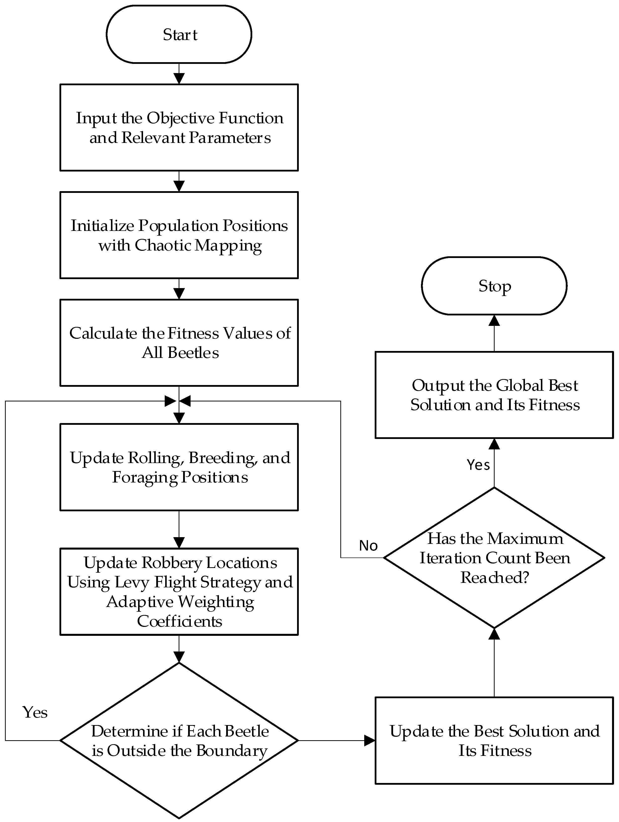
4. Fault Diagnosis Process for Parallel-Axis Gearboxes Based on WOA-VMD and t-SNE

4.1. Optimizing VMD with IDBO

The IDBO is utilized to optimize the number of modes (K) and penalty factor (α) in variational mode decomposition (VMD). The value of K significantly affects the effectiveness of the original data decomposition. A K value that is too large may lead to excessive decomposition, generating some ineffective intrinsic mode functions (IMFs), while a K value that is too small may result in insufficient decomposition of the original signal. The penalty factor α, when too large, can cause loss of frequency band signals, and, conversely, can introduce information redundancy. Therefore, an optimal combination of [K, α] is essential. In this study, the IDBO algorithm is employed to optimize the parameters of VMD. The optimization process aims to minimize the envelope entropy, which serves as the fitness function. Envelope entropy reflects the sparsity characteristics of the original signal. When there is more noise in the IMF and less feature information, the envelope entropy value is larger, and vice versa. The optimization process is as follows:

• Set the IDBO population size and the number of iterations, and define a suitable range for [K, α] values for VMD decomposition. Ensure that the range is not too narrow to avoid losing essential feature information in the modal components.
• Use VMD to decompose the vibration signal from the gearbox, resulting in several intrinsic mode functions (IMFs).
• Calculate the fitness function value for each set of [K, α] values and continually update the iterations to find the best fitness function value.
• Determine if the iteration is completed, i.e., whether the maximum number of iterations has been reached. When the maximum number of iterations is reached, terminate the iteration and save the optimal parameters [K, α].

4.2. Kurtosis-Based Signal Reconstruction

Kurtosis reflects the sharpness or peakedness of a signal waveform, and due to the varying impulsive components contained in each IMF, their corresponding kurtosis values are different [24]. When the kurtosis value K is 3, it corresponds to the normal kurtosis value for a Gaussian distribution curve, indicating that the IMF contains more fault-related information. Therefore, selecting kurtosis values greater than 3 implies a significant presence of signal impulses in the IMF, indicating that the vibration deviates from a normal state. This feature is suitable for identifying signal anomalies when faults occur.

4.3. Feature Extraction

Time domain features of vibration signals can reflect the overall state of the gearbox and can be used for fault detection and trend forecasting. Frequency domain features are useful for identifying the location and cause of faults. The combination of time and frequency domain feature information can effectively determine the current condition of the gears. In this paper, a variety of time domain and frequency domain feature parameters are selected to form the fault information feature matrix.

Information entropy describes the degree of uncertainty in a system and is used to analyze the complexity of a signal. Single entropy characteristics may not fully reflect the signal’s feature information. Therefore, multiple entropy values are extracted for each IMF to ensure data completeness and diagnostic accuracy. This paper extracts permutation entropy, fuzzy entropy, and sample entropy.

According to the above introduction, the specific steps for gear fault diagnosis based on IDBO-VMD decomposition, selection of IMF features, and t-SNE are as follows:

• Obtain vibration signals for various states using an accelerometer sensor.
• Use the IDBO algorithm to search the optimal parameters of VMD for each state. After parameter optimization, apply VMD to decompose the signals from various states, resulting in K IMF components.
• Apply the kurtosis criterion to filter the obtained IMF components, selecting the best IMF.
• Perform feature extraction on the chosen IMF, recombine the extracted 20 feature values to create a new feature vector.
• Utilize the t-SNE method for dimensionality reduction, obtaining a two-dimensional feature vector.
• Input the feature vectors of the training dataset into an SVM for training, creating an SVM classification model.
• Input the feature vectors of the testing dataset into the trained SVM model to perform fault diagnosis.

5. Simulation Testing

For testing the effectiveness of the proposed algorithm improvements, grey wolf optimization (GWO), DBO, the sparrow search algorithm (SSA), and IDBO were selected for comparative optimization on test functions. The test functions are listed in

Table 1. Test functions.

Test Functions	Dimension	Range	Optimal Value
$F_1\left(x\right)={\displaystyle \sum _{i=1}^n{x}_i^2}$	30	[−100, 100]	0
$F_2\left(x\right)={{\displaystyle \sum _{i=1}^n\left({\displaystyle \sum _{j-1}^i{x}_i}\right)}}^2$	30	[−100, 100]	0
$F_3(x)={\displaystyle \sum _{i=1}^n\left[100{\left(x_{i+1}-x_i^2\right)}^2+{\left(x_i-1\right)}^2\right]}$	30	[−30, 30]	0
$F_4\left(x\right)={\displaystyle \sum _{i=1}^n}-x_i\sin \left(\sqrt{\left|x_i\right|}\right)$	30	[−500, 500]	0
$F_5\left(x\right)=-20\exp \left(-0.2\sqrt{\frac{1}{n}{\displaystyle \sum _{i=1}^n{x}_i^2}}\right)-\exp \left(\frac{1}{n}{\displaystyle \sum _{i=1}^n\cos \left(2\pi x_i\right)}\right)+20+e$	30	[−32, 32]	0
$F_6\left(x\right)=\frac{\pi }{n}\left\{10\sin \left(\pi y_1\right)+{{\displaystyle \sum _{i=1}^n{\left(y_1-1\right)}^2\left[1+10{\sin }^2\left(\pi y_{1+i}\right)\right]}}^2\right\}+{\displaystyle \sum _{i=2}^{n}u\left(x_i,10,100,4\right)}$ $y_i=1+\frac{x_i+1}{4}$ $u\left(x_i,a,k,m\right)=\{\begin{array}{c}k{\left(x_i-a\right)}^m,x_i>a\\ 0,-a<x_i<a\\ k{\left(-x_i-a\right)}^m,x_i<-a\end{array}$	30	[−50, 50]	0

, where F₁–F₃ are single-peak functions, and F₄–F₆ are multipeak functions, all with a dimensionality of 30. To ensure fair testing, each algorithm utilized a population size of 30, a maximum iteration count of 500, and was independently tested on the six test functions 10 times to obtain average fitness convergence curves, evaluating their convergence speed. The experimental results are presented in Table 1, using criteria such as the best value, average value, and standard deviation for evaluation.

From Figure 3, it can be observed that under the same parameter settings, IDBO exhibits a faster convergence speed compared to DBO. In Figure 3c, the convergence speed of IDBO is slightly lower than DBO in the early stages, but it shows improvement in solution accuracy, and its average optimization capability is more stable. A comparison with GWO and SSA also reveals that DBO has good convergence speed and optimization capability. When comparing these four algorithms simultaneously, it is evident that IDBO’s convergence speed is significantly higher than the other three. Moreover, it requires the least number of iterations. As the iteration count increases, the convergence curves of DBO, the SSA, and GWO gradually stabilize, and optimization accuracy starts to decrease. This indicates that the three improvement strategies applied to IDBO result in a noticeable enhancement in convergence speed and an improvement in global search capability, showcasing the advantage in local optimization capability.

Table 2. Test results comparison.

	IDBO	DBO	GWO	SSA
F1
Optimal value	0	2.4081 × 10−176	5.5438 × 10−29	7.1886 × 10−100
Mean value	0	6.0809 × 10−107	6.7022 × 10−28	3.7487 × 10−60
Standard deviation	0	1.9229 × 10−106	1.3445 × 10−27	1.1854 × 10−59
F2
Optimal value	0	1.4802 × 10−76	4.9103 × 10−17	5.0108 × 10−81
Mean value	0	1.0308 × 10−58	8.2908 × 10−17	5.4129 × 10−32
Standard deviation	0	3.2597 × 10−58	2.9568 × 10−17	1.6937 × 10−31
F3
Optimal value	0	3.2393 × 10−76	2.2534 × 10−7	2.8709 × 10−93
Mean value	3.6372 × 10−90	1.8364 × 10−54	7.4764 × 10−7	7.0487 × 10−31
Standard deviation	1.1299 × 10−89	5.8014 × 10−54	5.1431 × 10−7	2.2202 × 10−30
F4
Optimal Value	0	4.3236 × 10−304	3.0912 × 10−53	5.4264 × 10−243
Mean Value	0	4.1335 × 10−210	1.7039 × 10−50	3.8374 × 10−124
Standard Deviation	0	0	3.7227 × 10−50	1.2135 × 10−123
F5
Optimal value	0	1.2767 × 10−162	7.9735 × 10−105	6.3863 × 10−119
Mean value	0	6.2664 × 10−114	3.5699 × 10−100	4.1615 × 10−44
Standard deviation	0	1.9816 × 10−113	9.4946 × 10−100	1.316 × 10−43
F6
Optimal value	4.4409 × 10−16	4.4409 × 10−16	7.5051 × 10−14	4.4409 × 10−16
Mean value	4.4409 × 10−16	4.4409 × 10−16	1.0134 × 10−13	4.4409 × 10−16
Standard deviation	0	0	3.8454 × 10−14	0

reveals that IDBO did not find the optimal solution only in the case of testing the F₆ function. Moreover, its performance in terms of average and standard deviation is similar to DBO. However, as shown in Figure 3, IDBO demonstrates the fastest convergence speed, swiftly locating the optimal values and exploring them in-depth, showcasing higher optimization accuracy. For the F₁–F₅ tests, IDBO outperforms other algorithms, showing significant improvements in average optimization capability, precision, and standard deviation. In summary, in the convergence curves of most test functions, the IDBO algorithm exhibits excellent performance. It maintains an absolute advantage in convergence speed while achieving high convergence accuracy, reflecting a reasonable balance between global search capability and local development capability.

6. Experimental Verification

6.1. Description of Experimental Data

This experiment adopted the data of condition monitoring and the fault diagnosis comprehensive test bench produced by Houde Company in Jiangsu, China for experimental verification, and the experimental equipment is shown in Figure 4. Four prevalent fault states were selected, namely, normal gear state, tooth root fracture, tooth surface wear, tooth surface pitting, and tooth surface cracking. Multiple sets of vibration signals under different states were acquired using acceleration sensors. The gearbox features oil-immersed lubrication, with the motor speed set to 1800 r/min, a sampling frequency of 12 kHz, a sampling duration of 10 min, and a sample length set to 1024. This resulted in 50 sample sets for each state, amounting to a total of 250 sample sets, with 200 sets designated for training and 50 sets for testing.

6.2. The Extraction of Fault Signal Features

Using envelope entropy as the fitness value, we compared the fitness curves of the IDBO, DBO, SSA, and GWO algorithms in optimizing VMD. To ensure fair testing, each algorithm was configured with 30 individuals, a maximum iteration count of 50, and a range of values for K set to [3, 10], all of which are integers. The penalty factor α had a value range of [200, 5000]. In Figure 5, each curve represents the optimization iteration process for VMD using the four algorithms.

From Figure 5, it can be observed that GWO has the highest fitness values in the signal decomposition of the four types of fault signals. This indicates that GWO has poor global search capability and is prone to becoming stuck in local optima. DBO, the SSA, and IDBO have lower fitness values than GWO, indicating stronger global search capabilities. However, with the increase in iteration count, GWO exhibits strong convergence ability. Through comparison, it is evident that IDBO has lower fitness values, attributed to the cubic chaos mapping’s ability to quickly locate global optimal solutions. With iterations, IDBO can rapidly find the lowest fitness value. This is due to the inclusion of the Levy flight strategy and adaptive weighting, which enhance global optimization capability and convergence performance. The optimization facilitated by IDBO improves the robustness of VMD, effectively suppresses modal aliasing, and rapidly identifies the optimal values for parameters K and α. The fitness value used for testing is the minimum envelope entropy. The smaller the value, the less noise contained in the IMFs obtained from VMD, allowing for the extraction of more fault features. Therefore, IDBO enhances the robustness of VMD, effectively suppressing modal aliasing, and rapidly determining the optimal values for parameters K and α. This contributes to the improved ability to extract fault features by minimizing noise interference in the VMD decomposition process.

Taking the surface crack fault signal as an example, the iteration curve of the VMD parameter optimization process is shown in Figure 6. After 10 iterations, the global optimal solution was found, resulting in the minimum envelope entropy of 4.2092. The optimal solution corresponds to parameters α = 741 and K = 5. Subsequently, using VMD processing, the signals and spectra corresponding to the five intrinsic mode functions (IMFs) of the surface crack fault signal are shown in Figure 7 and Figure 8.

The optimal parameter combinations for VMD were determined for the five different states, as shown in

Table 3. Optimal parameter.

Gear Condition	[K, α]
Normal condition	[6, 2232]
Tooth root breakage	[5, 648]
Surface pitting	[4, 476]
Surface cracking	[5, 741]
Surface wear	[4, 2678]

.

Based on the parameter combinations [K, α] from Table 3, the VMD method was configured with the appropriate values of K and α, and this was used to decompose the samples into multiple intrinsic mode function (IMF) components.

Table 4. Kurtosis values of five signal IMF components.

State	IMF1	IMF2	IMF3	IMF4	IMF5	IMF6
Normal	3.25	4.29	3.82	4.20	3.49	3.89
Breakage	2.44	2.95	3.20	2.89	4.26
Pitting	3.15	3.44	3.58	4.41
Cracking	2.66	4.13	3.25	4.84	5.22
Wear	2.89	13.95	15.22	8.79

presents the kurtosis values for each IMF corresponding to each state. Larger kurtosis values indicate greater impulsive characteristics in the components and, therefore, more distinctive features within the fault signal. The four IMFs with the highest kurtosis values were selected for each state, and 20 vibration features were extracted from each, resulting in a total of 80 features for each segment of the vibration signal, forming high-dimensional feature vectors.

6.3. t-SNE Dimensionality Reduction Effect

To validate the dimensionality reduction effect of t-SNE, this study selected the Iris dataset provided by the SKLearn library for dimensionality reduction. The Iris dataset consists of three different species of iris flowers, with 150 samples for each flower type and four features for each sample. The PCA, LLE, and t-SNE algorithms were used for dimensionality reduction, and the visualization results of each method are shown in Figure 9.

From Figure 9, it is evident that, through dimensionality reduction of the Iris flower dataset, PCA exhibits a suboptimal intraclass clustering effect. LLE, while preserving the inherent manifold structure, fails to separate different types effectively, resulting in poor intraclass clustering. Conversely, after dimensionality reduction using t-SNE, there is noticeable intraclass cohesion and interclass separation, rendering it the most visually effective. Although t-SNE does not exhibit a significantly superior separation of different types compared to PCA, it notably outperforms PCA in terms of intraclass cohesion. Therefore, t-SNE was chosen for dimensionality reduction of the fault dataset.

6.4. Fault Feature Dimensionality Reduction

Feature information extraction is a crucial step in gearbox fault diagnosis. Using permutation entropy, fuzzy entropy, and sample entropy, the entropy features and time–frequency domain features of the main intrinsic mode functions (IMFs) were extracted to construct the initial feature vector. However, the obtained initial feature vector may have high dimensionality and could contain redundant features. Therefore, normalization was applied to the extracted data, and the t-SNE algorithm was utilized to reduce the dimensionality of high-dimensional feature vectors to obtain low-dimensional feature vectors. Additionally, the PCA and LLE methods were employed for dimensionality reduction, and the results of the dimensionality reduction are illustrated in Figure 10.

From Figure 10, Figure 10b illustrates the dimensionality reduction effect of LLE, showing poor performance as it fails to effectively separate different fault types. Although PCA can separate the fault types, its clustering is poor, and it cannot perfectly isolate the fault types. Through the comparison of the three dimensionality reduction methods, t-SNE exhibits the best dimensionality reduction effect. It can completely separate the five states, with the best clustering, distinct feature differentiation, and the ability to maximize the preservation of the original matrix’s characteristics. Therefore, t-SNE was chosen for dimensionality reduction, resulting in two-dimensional feature vectors.

6.5. Fault Classification

The feature vectors of the 200 training samples were input to the SVM classifier for training, resulting in an SVM model for fault diagnosis. Subsequently, the 50 test samples were input into the trained SVM model for classification. In the SVM training and testing, numeric labels were used to represent the five gear operating states: normal state as label 0, tooth root fracture as label 1, surface wear as label 2, surface cracking as label 3, and surface pitting as label 4. The diagnostic accuracy for gear classification can reach 100% using the IDBO-VMD and t-SNE dimensionality reduction feature extraction methods.

To demonstrate the accuracy of the proposed approach, the same collected data were used, and signal decomposition was performed using three methods: EMD, traditional VMD, and IDBO-VMD. For traditional VMD, the parameter selection was based on the central frequency method, where the final value of K was determined by observing the central frequencies of IMF components for different K values [25]. K = 6 and α = 2000 were confirmed through observation.

Then, feature extraction and t-SNE dimensionality reduction were carried out, and, finally, the obtained low-dimensional feature distribution and SVM classification accuracy are depicted in Figure 9 and presented in

Table 5. SVM classification accuracy of three methods.

Method	Classification Accuracy/%
EMD + t-SNE	95
VMD + t-SNE	98
IDBO-VMD + t-SNE	100

, respectively.

According to Figure 11 and Table 5, it is evident that the diagnostic accuracy using the feature extraction method based on IDBO-VMD and t-SNE is slightly higher than the other two methods. Furthermore, the fault features obtained through EMD decomposition and t-SNE dimensionality reduction are effective in separating the four different states, but the clustering effect is suboptimal. From Figure 12, it can be observed that both EMD and traditional VMD exhibit diagnostic errors when diagnosing normal signals, leading to a decrease in accuracy. Therefore, the proposed IDBO-VMD and t-SNE methods, characterized by high accuracy and ease of operation, represent effective approaches for fault diagnosis.

7. Conclusions

In this paper, we proposed a novel approach for gearbox fault diagnosis. We enhanced the DBO algorithm and compared it with DBO, the SSA, and GWO. The introduced IDBO algorithm demonstrated excellent performance, whether applied to benchmark functions or utilized in optimizing VMD. The algorithm exhibited strong global optimization capabilities and convergence performance. Additionally, it boasts fast training speeds, straightforward operations, and high optimization accuracy, showcasing its efficiency in the context of mechanical applications.

Experimental results demonstrate that the VMD optimized using IDBO effectively suppresses mode mixing. By employing the IDBO-VMD and t-SNE feature extraction methods, the low-dimensional vectors obtained were input to an SVM for gearbox fault diagnosis, achieving an accuracy rate of 100%. Compared to traditional methods, this approach exhibits characteristics such as high fault recognition accuracy and stable performance, making it an effective new method for gearbox fault diagnosis. Currently, the proposed method has only been applied to gearbox diagnosis, and future work will involve extending its application to diagnose faults in other rotating machinery, thus validating its practicality and generality.

References

1. Vachtsevanos, G.J.; Lewis, F.; Roemer, M.; Hess, A.; Wu, B. Intelligent Fault Diagnosis and Prognosis for Engineering Systems; John Wiley & Sons, Inc.: Hoboken, NJ, USA, 2006. [Google Scholar]
2. Hirani, H.; Athre, K.; Biswas, S. Comprehensive Design Methodology for an Engine Journal Bearing. Proc. Inst. Mech. Eng. Part J J. Eng. Tribol. 2000, 214, 401–412. [Google Scholar] [CrossRef]
3. Hotait, M.A.; Kahraman, A. Experiments on the Relationship between the Dynamic Transmission Error and the Dynamic Stress Factor of Spur Gear Pairs. Mech. Mach. Theory 2013, 70, 116–128. [Google Scholar] [CrossRef]
4. Kahraman, A. Effect of axial vibrations on the dynamics of a helical gear pair. J. Vib. Acoust. 1993, 115, 33–39. [Google Scholar] [CrossRef]
5. Li, Z.; Zhang, T.; Chen, Y.; Song, L. The Effect of Parallel-Axis Helix Gear Pair on Wind Turbine Gearbox Vibration Control. Shock. Vib. 2020, 2020, 8893890. [Google Scholar] [CrossRef]
6. Huang, E.N.; Shen, Z.; Long, R.S.; Wu, M.C.; Shih, H.H.; Zheng, Q.; Yen, N.C.; Tung, C.C.; Liu, H.H. The Empirical Mode Decomposition and the Hilbert Spectrum for Nonlinear and Non-Stationary Time Series Analysis. Proc. Math. Phys. Eng. Sci. 1998, 454, 903–995. [Google Scholar] [CrossRef]
7. Zhang, Y.T.; Li, C.L.; Jiang, Y.Q.; Sun, L.; Zhao, R.B.; Yan, K.F.; Wang, W.H. Accurate prediction of water quality in urban drainage network with integrated EMD-LSTM model. J. Clean. Prod. 2022, 354, 131724. [Google Scholar] [CrossRef]
8. Deng, Y.; Zhu, K.H.; Zhao, G.J.; Zhu, J.Y. Efficient partial discharge signal denoising method via adaptive variational modal decomposition for infrared detectors. Infrared Phys. Technol. 2022, 125, 104230. [Google Scholar] [CrossRef]
9. Dragomiretskiy, K.; Zosso, D. Variational Mode Decomposition. IEEE Trans. Signal Process. 2014, 62, 531–544. [Google Scholar] [CrossRef]
10. Zhan, J.; Cheng, L.; Peng, Z. Based on VMD and Improved Multi-Classification Matian Series Integrated Intelligent Diagnosis of Rolling Bearing Faults. Vib. Shock 2020, 39, 32–39. [Google Scholar]
11. Tang, G.; Wang, X. Parameter Optimized Variational Mode Decomposition Method with Application to Incipient Fault Diagnosis of Rolling Bearing. J. Xi’an Jiaotong Univ. 2015, 49, 73–81. [Google Scholar]
12. Ding, J.; Wang, Z.; Yao, L.; Cai, Y. Rolling Bearing Fault Diagnosis Based on GCMWPE and Parameter Optimization SVM. China Mech. Eng. 2021, 32, 147–155. [Google Scholar] [CrossRef]
13. Shen, T.; Huang, S.; Han, S. Extracting Information Entropy Features for Rotating Machinery Vibration Signals. Chin. J. Mech. Eng. 2001, 37, 94–98. [Google Scholar] [CrossRef]
14. Li, Y.; Li, Y.; Chen, X.; Wei, J. Feature Extraction and Classification of Ship Radiated Noise Based on VMD and SVM. J. Natl. Univ. Def. Technol. 2019, 41, 89–94. [Google Scholar]
15. Li, Z.; Jiang, Y.; Guo, Q.; Hu, C.; Peng, Z. Multi-dimensional Variational Mode Decomposition for Bearing-Crack Detection in Wind Turbines with Large Driving-Speed Variations. Renew. Energy 2018, 116, 55–73. [Google Scholar] [CrossRef]
16. Wang, C.; Li, H.; Huang, G.; Ou, J. Early Fault Diagnosis for Planetary Gearbox Based on Adaptive Parameter Optimized VMD and Singular Kurtosis Difference Spectrum. IEEE Access 2019, 7, 31501–31516. [Google Scholar] [CrossRef]
17. Zhang, M.; Jiang, Z.; Feng, K. Research on Variational Mode Decomposition in Rolling Bearings Fault Diagnosis of the Multistage Centrifugal Pump. Mech. Syst. Signal Process. 2017, 93, 460–493. [Google Scholar] [CrossRef]
18. Xue, J.; Shen, B. Dung Beetle Optimizer: A New Meta-Heuristic Algorithm for Global Optimization. J. Supercomput. 2022, 79, 7305–7336. [Google Scholar] [CrossRef]
19. Ge, Y.; Guo, L.Z.; Niu, S.G.; Dou, Y. Prediction of Remaining Useful Life Based on t-SNE and LSTM for Rotating Machinery. J. Vib. Shock 2020, 39, 223–231. [Google Scholar]
20. Zhang, J.; Zheng, J.; Xie, X.; Lin, Z.; Li, H. Mayfly Sparrow Search Hybrid Algorithm for RFID Network Planning. IEEE Sens. J. 2022, 22, 16673–16686. [Google Scholar] [CrossRef]
21. Feng, J.; Zhang, J.; Zhu, X.; Lian, W. A Novel Chaos Optimization Algorithm. Multimed. Tools Appl. 2017, 76, 17405–17436. [Google Scholar] [CrossRef]
22. Reynolds, A. Cooperative Random Levy Flight Searches and the Flight Patterns of Honeybees. Phys. Lett. A 2006, 354, 384–388. [Google Scholar] [CrossRef]
23. Yang, C.-Y.; Ma, Y.-W.; Chen, J.-L.; Lin, C.-J.; Lee, W.-L. Novel Dynamic KNN with Adaptive Weighting Mechanism for Beacon-Based Indoor Positioning System. J. Internet Technol. 2019, 20, 1601–1610. [Google Scholar]
24. Hu, A.J.; Ma, W.L. Rolling Bearing Fault Feature Extraction Method Based on Ensemble Empirical Mode Decomposition and Kurtosis Criterion. Proc. CSEE 2012, 32, 106–111+153. [Google Scholar]
25. Liu, C.L.; Wu, Y.J.; Zhen, C.G. Rolling Bearing Fault Diagnosis Based on Variational Mode Decomposition and Fuzzy C-Means Clustering. Proc. CSEE 2015, 35, 3358–3365. [Google Scholar]
Figure 1. Scatter diagram and distribution histogram of the chaotic sequences generated using cubic chaos map. (a) Iteration; (b) chaotic Sequences.
Applsci 14 00289 g001
Figure 2. Improved dung beetle algorithm flowchart.
Applsci 14 00289 g002
Figure 3. Convergence curves of functions F1 to F6: (a) F1; (b) F2; (c) F3; (d) F4; (e) F5; (f) F6.
Applsci 14 00289 g003
Figure 4. Experimental equipment: (a) gearbox; (b) surface pitting; (c) surface cracking; (d) surface wear; (e) tooth root breakage.
Applsci 14 00289 g004
Figure 5. Fitness curves for optimizing VMD using different algorithms: (a) normal condition; (b) tooth root breakage; (c) surface cracking; (d) surface pitting.
Applsci 14 00289 g005
Figure 6. Iteration count.
Applsci 14 00289 g006
Figure 7. Gear surface crack fault signal waveform.
Applsci 14 00289 g007
Figure 8. Gear surface crack fault signal spectrum.
Applsci 14 00289 g008
Figure 9. Visualization of dimensionality reduction methods: (a) t-SNE; (b) PCA; (c) LLE.
Applsci 14 00289 g009
Figure 10. Comparison of three dimensionality reduction methods: (a) t-SNE dimensionality reduction effect; (b) dimensionality reduction effect; (c) PCA dimensionality reduction effect.
Applsci 14 00289 g010
Figure 11. Low-dimensional feature distribution: (a) IDBO-VMD + t-SNE; (b) EMD + t-SNE; (c) VMD + t-SNE.
Applsci 14 00289 g011
Figure 12. Confusion matrix: (a) EMD + t-SNE; (b) IDBO-VMD + t-SNE; (c) VMD + t-SNE.
Applsci 14 00289 g012