Article

EEG Emotion Classification Based on Graph Convolutional Network

1
Artificial Intelligence Institute of China Electronics Technology Group Corporation, Beijing 100041, China
2
Beijing Institute of System Engineering, Beijing 100101, China
3
State Key Laboratory of Software Development Environment, Beihang University, Beijing 100191, China
*
Author to whom correspondence should be addressed.
Appl. Sci. 2024, 14(2), 726; https://doi.org/10.3390/app14020726
Submission received: 1 September 2023 / Revised: 23 September 2023 / Accepted: 16 October 2023 / Published: 15 January 2024
(This article belongs to the Special Issue Methods and Applications of Data Management and Analytics)

Abstract

:
EEG-based emotion recognition is a task that uses scalp-EEG data to classify the emotion states of humans. The study of EEG-based emotion recognition can contribute to a large spectrum of application fields including healthcare and human–computer interaction. Recent studies in neuroscience reveal that the brain regions and their interactions play an essential role in the processing of different stimuli and the generation of corresponding emotional states. Nevertheless, such regional interactions, which have been proven to be critical in recognizing emotions in neuroscience, are largely overlooked in existing machine learning or deep learning models, which focus on individual channels in brain signals. Motivated by this, in this paper, we present RGNet, a model that is designed to learn the regional level representation of EEG signal for accurate emotion recognition. Specifically, after applying preprocessing and feature extraction techniques on raw signals, RGNet adopts a novel region-wise encoder to extract the features of channels located within each region as input to compute the regional level features, enabling the model to effectively explore the regional functionality. A graph is then constructed by considering each region as a node and connections between regions as edges, upon which a graph convolutional network is designed with spectral filtering and learned adjacency matrix. Instead of focusing on only the spatial proximity, it allows the model to capture more complex functional relationships. We conducted experiments from the perspective of region division strategies, region encoders and input feature types. Our model has achieved 98.64 % and 99.33 % for Deap and Dreamer datasets, respectively. The comparison studies show that RGNet outperforms the majority of the existing models for emotion recognition from EEG signals.

1. Introduction

Emotion recognition has gained increasing prominence in many areas, such as human–computer interaction and healthcare. For instance, developing the ability to recognize emotion can assist in understanding the emotional states of patients. Existing techniques for emotion recognition can be categorized into non-physiological methods and physiological methods. The non-physiological methods involve facial expression, speech, eye movement and so on [1,2,3,4]. A main issue with the non-physiological method is its uncertainty and unreliability, as humans can deliberately conceal their true emotions. On the other hand, the physiological methods offer a higher degree of objectivity since they produce uncontrollable physiological responses, providing a potentially more accurate reflection of emotional states. Electroencephalography (EEG), as one of the physiological methods, has been widely used in emotion recognition tasks due to its easy acquisition and high temporal resolution. The collection of EEG signal is carried out by placing the electrodes on a human scalp to record the electrical activity of underlying brain tissues. As the production of emotion tends to have a strong connection with the activity within brain structures that can be captured by electrograms, the investigation of EEG signal can help to explore this functionality, exemplifying the importance of conducting research on emotion recognition using EEG signals. Nowadays, the processing and classification on EEG data still remains challenging. Essentially, EEG signal is the observation of source signal that has been sent from deeper brain regions that varies with time and is transmitted with different intensity. This non-stationary property makes it difficult to be handled by linear methods [5]. Moreover, EEG signal can be contaminated with noise and artifacts produced by the external environment or mixed with other signals. These issues may affect the collection of brain signals, making it challenging to handle emotion classification by naive methods. Therefore, more and more studies are seeking machine learning or deep learning approaches to solve this task.
Earlier studies primarily emphasize how to extract temporal features from an individual channel, where the inter-channel activity was not thoroughly explored [6,7,8]. Recently, there have been many works proposed to utilize the fused features of multiple channels. For instance, some studies utilizing convolutional neural networks (CNNs) combine the signal with adjacent channels by treating electrodes as equally spaced pixels in images; another widely used approach is graph neural networks (GNNs), which map channels into nodes and relationships into edges to probe the topological characteristics of brain activity. Although these formulations provide a way to describe how activities from different locations occur coherently by channel-level representation, it still does not guarantee to capture the complex functional relationship occurring at the regional level, which has been identified to be an important factor in the elicitation of emotion. Studies in neuroscience reveal that the functionality of brain regions and their interactions are important factors in the process of emotion production [9,10,11,12]. Extracting interactions and features frim regions rather than channels allows us to follow the nature of brain structures and has the potential to create the ability to interpret the association between brain activity and emotion states.
Based on such a point, there are several works proposed to tackle emotion recognition from the perspective of brain regions. Ref. [13] uses Bi-LSTM to capture the regional feature and global feature; Refs. [14,15] focus on extracting features for hemisphere. Although these approaches develop effective ways to present regional features, they do not thoroughly investigate the topological structure and interactions among brain regions. Ref. [16] addresses this issue by constructing local and global graphs. However, it takes the assumption that the connection only exists between nodes or regions that have similar characteristics, which limits the scope on investigating the complex structure of regions.
In this study, we propose a model that investigates both the internal and the global activity of brain regions to identify emotions. Our model firstly adopts a preprocessing technique and feature extractions on the input EEG signal. Next, the channels within the same region are grouped together to form regional data. The region encoder is applied to extract the representative features of each region. For the purpose of learning topological structure among different regions, the graph convolutional network (GCN) is employed to learn more discriminative features. The main contributions of our study include:
  • We propose a model that solves emotion recognition based on region-level representation to learn the activity inside and across various brain regions. Such interactions have been proven to be highly relevant to human emotion state from a neurological point of view.
  • To capture the correlation between brain regions, we construct a graph on EEG signals and employ graph spectral filtering with dynamical adjacency matrix. This approach is more applicable to study the interplay of brain areas since it does not limit itself to the notion of geographic closeness and provides flexibility in detecting function-level interactions.
  • To thoroughly investigate how to formulate regional-level characteristics, we conduct a comprehensive experimental study in terms of different region encoders, region division strategies and input features. The results show that our approach outperforms many existing methods on DEAP and Dreamer datasets.

2. Literature Review

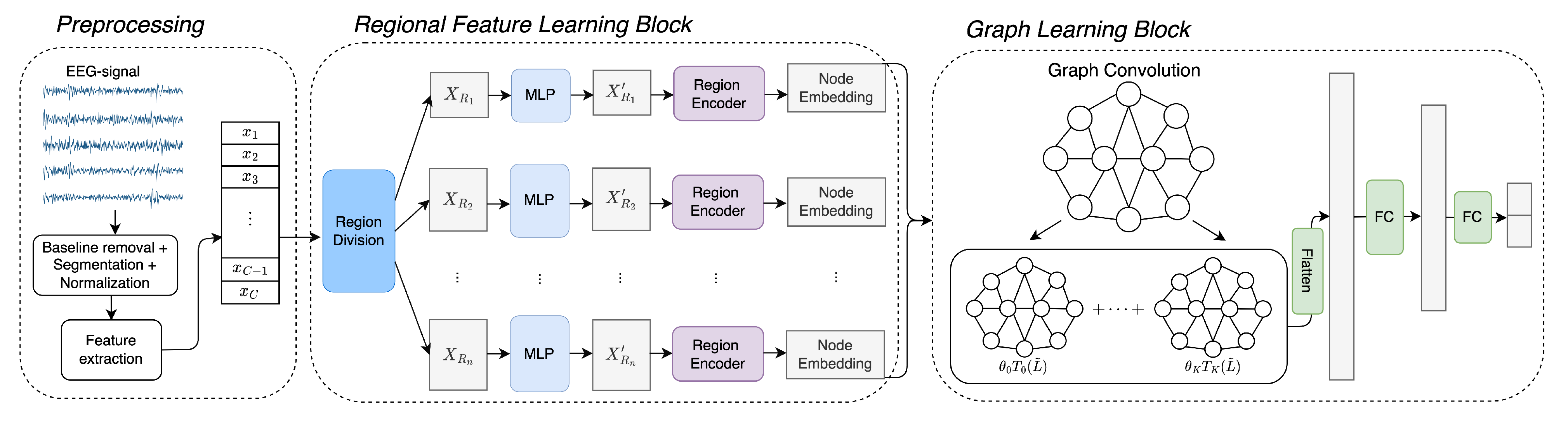
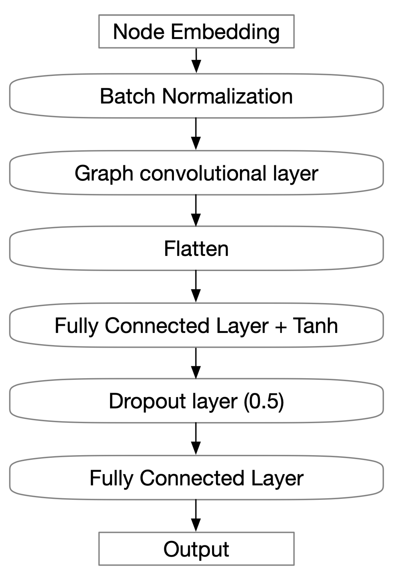
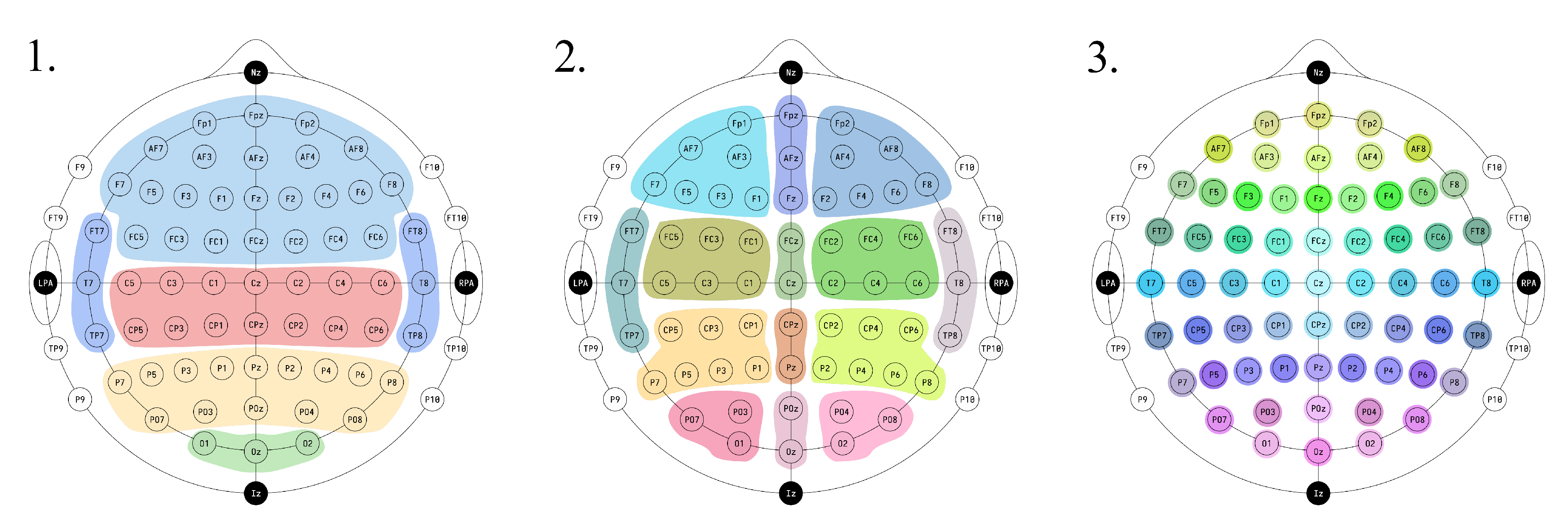
Due to the dynamics property and noise presented in an EEG signal, EEG-based emotion recognition has always been a challenging task. Many researchers have employed a wide range of methods to tackle this problem. In this section, we introduce the works that mainly utilize machine learning and deep learning approaches.

2.1. Machine Learning Approach

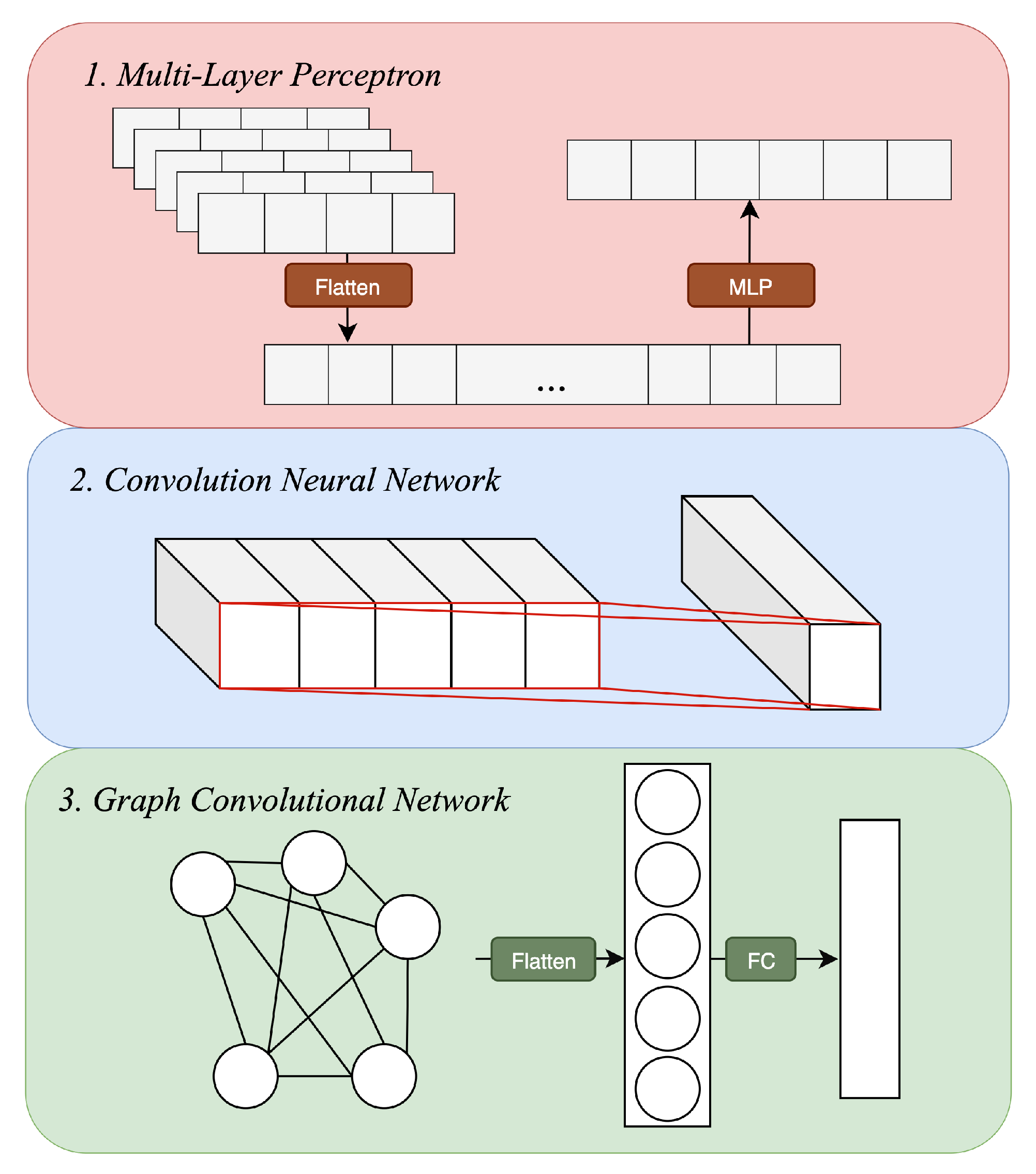
Machine learning is a widely used approach in EEG emotion recognition. It often starts with preprocessing the raw signal and extracting hand-crafted features. Then, features are fed into a machine learning model, such as a support vector machine, K-nearest neighbor, decision tree, etc., to classify emotion states.
Many studies have been carried out that focus on evaluating the effectiveness of different features. Ref. [17] explores power spectral density, differential asymmetry and rational asymmetry of the paired channels under multiple frequency bands. These features are processed by a support vector machine to recognize emotions. It finds that differential asymmetry is more robust to detect the brain dynamics caused by emotions. Moreover, information provided by the channels from the frontal and parietal lobe is useful to distinguish emotions. Ref. [18] conducts studies on emotion classification with different features as input. During the process, feature dimensionality reduction techniques, such as principal component analysis and linear discriminant analysis, are adopted to improve the efficiency and accuracy. The experiment results indicate that the power spectrum was identified as the most effective amongst all input features and the high frequency band tends to be more useful in emotion classification. These studies show that the choice of input features can largely affect the results.
To compare which classifiers have the best performance, Ref. [6] utilizes statistical data, i.e., min, max, mean and standard deviation, as the input. Then, it adopts a K-nearest neighbor, regression tree, Bayesian network, support vector machine and artificial neural network for classification. The experiments show that the K-nearest neighbor and support vector machine give the best results among all the models. However, it can be challenging for the majority of machine learning methods to work well with large datasets. Ref. [19] employs discrete wavelet transform and spectral features. In the classification stage, it applies a support vector machine with the aid of a radial basis function kernel to process features from 10 channels to do the classification. Ref. [20] employs empirical mode decomposition/intrinsic mode functions and variational mode decomposition to process the raw EEG signal which is widely used in biomedical studies. These methods are used to decompose nonlinear and non-static signals and feed them into VMD to identify low and high frequencies. Then, it extracts two non-linear features: entropy and Higuchi’s fractal dimension. Finally, it carries out experiments by using Naive Bayes, K-nearest neighbor, decision tree and convolutional neural networks to recognize emotions. A common observation from these studies is that the support vector machine often generates the best outcomes in emotion classification tasks.

2.2. Deep Learning Approach

Recently, extensive research efforts have been devoted to deep learning techniques for EEG-based emotion identification due to the robustness and low requirement for prior knowledge. These techniques can be generally classified according to the type of network used, as those with similar architectures are prone to follow analogous ideas.
In previous studies, a common class of deep learning model to address EEG-based emotion classification is long-short term memory (LSTM), which is typically designed to capture temporal dependencies with data sequences. Ref. [21] directly inputs EEG signal into the LSTM network by treating channels as features for each time frame. Similarly, Ref. [7] computes the discrete wavelet transform from the raw signal, followed by the extraction of statistical data. These extracted features are then fed into a network architecture that combines LSTM layers with dense layers for each individual channel. Ref. [15] further extends LSTM with a domain adversarial neural network. It involves the extraction of features from each hemisphere using an LSTM-based approach. The domain adversarial network is adopted here to address the challenge of cross-subject variability. These studies demonstrate the strength of LSTM in effectively capturing temporal characteristics from EEG data. A potential drawback of LSTM is that it may hinder the ability to learn the spatial connections among EEG channels.
Another type of network widely adopted in emotion recognition with EEG signal is a convolutional neural network (CNN), which uses a shared-weight kernel to slide over data. It is primarily utilized in the area of image analysis due to its advantages for processing data with grid patterns. Ref. [22] examines the power of CNN in terms of architecture, design and training decisions. The results indicate that CNN is capable of learning highly discriminative features when given the proper conditions. Ref. [23] adopts a 3D convolution layer, which is able to learn spatial and temporal features simultaneously. It requires a 3D input representation for the EEG signal by appending consecutive frames together. Ref. [24] develops a compact convolution architecture for EEG-based brain–computer interfaces (BCI). It introduces separable and depthwise convolution, which can not only give extract interpretable features but also reduces the number of parameters. Ref. [14] uses multi-scale convolutional layers to extract temporal and spatial layers. It specifically considers the asymmetrical property in the frontal area of brain. These studies demonstrate that CNN is capable of processing both temporal and spatial aspects of EEG signals. However, an issue that often comes with CNN is the inflexibility when considering the relationships among channels or areas. As the nature of CNN is to presume the grid pattern of input data, it is challenging for CNN to investigate non-Euclidean connectivity. On the other hand, this problem can be handled by a graph-based approach.
A graph neural network (GNN) is a class of networks that presents data in a graph structure. In EEG signal tasks, a graph is often constructed by treating each channel as a node, while the formulation of edges could vary. One of the options is to utilize the spatial proximity. Ref. [25] builds a 2D matrix to mark the relative position of electrodes. Then, the adjacency matrix is obtained by thresholding the shortest distance between a node and its neighbors. Ref. [26] establishes the connectivity based on the inverse square function of the physical distance. However, argued by [27], these spatial-based formulations may not represent the real functional connection between channels. To address this problem, it proposes a dynamical graph convolutions neural network that can dynamically learn the intrinsic relationship between nodes. In those works that employ GNN, the advantage of exploring topological structure makes it more adaptable to investigate the relationship between channels.
To improve the performance on both the spatial and temporal level, hybird networks are used that are composed of different types of networks. From the perspective of signal decomposition, Ref. [28] proposes a model that derives the source signal by stack autoencoder (SAE). Next, the sequenced features are fed into the LSTM network to learn the contextual correlation. Ref. [29] proposes a model that first captures spatial features by convolution layers at each timestamp and feeds them into the LSTM layer. The novelty in this work is that it adopts an attention mechanism in both stages to capture which channel or which timestamp contributes more in the process of emotion recognition. Ref. [30] employs a combination of GNN and LSTM, where GNN is responsible for learning static graph-domain features and LSTM extracts effective information from the channel-level relationships in a short range of time. Recently, the study of spatial-temporal graph learning has also been employed in EEG emotion classification. Ref. [31] integrates the spatial graph convolutional network with an attention-enhanced bi-directional LSTM module. This type of model better combines the temporal information to learn the features.
In addition to the aforementioned approach, some other novel methods have emerged in the field of EEG-based emotion classification. The methods provide different directions for advancing the deep learning techniques on EEG emotion classification. One of these methods, Ref. [32], focuses on a real-time method, which employs online learning techniques, including adaptive random forest, streaming random patches and logistic regression. Ref. [33] utilizes a capsule network to extract hierarchical features from the EEG signal, where each emotional capsule associates with an individual task. To enhance the power of multi-task learning, it uses the dynamic routing algorithm to achieve information exchange between primary capsules and emotional capsules. Recently, reinforcement learning has gained attention in EEG emotion classification as well. An example is [34], which is a reinforcement learning-based method that combines the idea of Papez circuit theory and uses EEG signals from the frontal lobe to simulate brain mechanisms. The key contribution in this approach is the utilization of a double dueling deep Q network, which enhances the decision-making process with more informed choices. These various methods have significantly advanced the field of deep learning for EEG emotion classification.

3. Method

In this paper, we propose a deep learning model, RGNet, to address the emotion recognition task. The structure of our model is shown in Figure 1. We firstly present the preprocessing technique in Section 3.1. Next, we introduce the regional feature learning block, which attempts to learn the region functionality in Section 3.2. Finally, to capture the interactions between regions, the graph learning block is proposed in Section 3.3.

3.1. Prepocessing

In order to retrieve useful signals that correspond to the emotions elicited by stimuli, we adopt several preprocessing techniques: the baseline signal removal method [35], segmentation and normalization.
Given the trial signal denoted by X R C × T , where C is the number of channels and T is the time duration, assume the time duration in seconds is t and the frequency of signal is f, then by the definition of frequency, we have T = t × f . It suggests that signal X can be split up into t segmentations where we denote each segmentation as X i R C × f . Similarly, the baseline signal X b can be segmented into t b signals where the i t h segmentation is referred to as X i b R C × f . The mean of baseline signal X ¯ b can be derived as following:
X ¯ b = i = 1 t b X i b t b .
Next, X ¯ b will be subtracted from each segmentation of the trial signal:
X i = X i X ¯ b .
The normalization is then applied, i.e., X i is subtracted by its mean and divided by the standard deviation. Once the preprocessing is completed, we further extract features for each slice. The details of segmentation and feature extraction are described in Section 4.

3.2. Regional Feature Learning Block

Many studies have argued that individual emotions can be related to activity in multiple brain regions and a single region can be associated with the formulation of multiple emotions [12,36,37,38]. It is therefore vital to investigate the function that each region plays to determine how the activity of each region helps to recognize different emotions. In this study, we intend to explore the emotional functionality of brain regions by gathering channels within the same region and then feeding them into the corresponding region encoder.
Based on the spatial location of channels, we divide EEG channels into n different regions R 1 , R 2 , , R n , where R i is defined as a set of channels grouped together, i.e., R i = { k 1 , k 2 , , k m } , and k j refers to the channel index. The regional input X R i R m × T s consists of the signals of channels in the same region:
X R i = { x k j | x k j R 1 × T s , k j R i } ,
where x k i is the signal of channel k i . Firstly, we apply a multi-layer perceptron (MLP) to process the raw input signal X R i R m × T s :
X R i = M L P ( X R i ) .
The processed data X R i R m × F i n will be taken as the input to be fed into the region encoder f i :
F R i = f i ( X R i ) , i { 1 , 2 , , n } .
The structure of region encoder f i is displayed in the third section in Figure 2. We employ the graph-based network by mapping channels into nodes. The benefit of this approach is its ability to model the underlying patterns of each region since it provides a natural way to explore the relationships between channels, rather than focusing on the integration of individual channel features. In the graph, all nodes are fully connected to each other at the beginning due to the observation that channels in the same region tend to have similar activities. We adopt a graph convolutional network (GCN) to propagate the information among nodes. Finally, the derived node features are flattened and passed into fully connected layers to produce the output F R i . The detail of the GCN is described in Section 3.3.

3.3. Graph Learning Block

Many works suggest that the correlation of regional brain activation plays a critical role in the processing of emotions [12,39]. Thus, with given features of an individual region, we seek a method that allows the study of how these regions relate to one another. In neuroscience research, graph theoretic analyses are frequently employed to investigate functional brain networks from a topological standpoint since they provide a systematic approach to analyze brain structure by mapping neural elements into nodes and their connections into edges [40,41,42]. Following such an idea, we feed the regional features derived from the region encoder into a graph convolutional network (GCN). We employ the spectral approach to define the convolutional filter instead of spatial approach since it is the more dominant method for dealing with signal processing [43].
The regional features derived from Section 3.2 are used as nodes to formulate a graph G . Then, assume we have the graph G with adjacency matrix A R n × n and degree matrix D R n × n . We can derive the Laplacian matrix by L = D A , or the normalized version L ^ = I D 1 2 A D 1 2 . Since L will be a real symmetric positive semidefinite matrix, it can be decomposed into
L = U Λ U T
via singular value decomposition where λ = d i a g ( λ 1 , , λ n ) is the diagonal matrix of the eigenvalues of L ^ and U is the Fourier basis. For a given graph data point X, we can derive its graph Fourier transform and inverse graph Fourier transform:
X ^ = U T X ,
X = U X ^ .
Then, the signal filtered by function g θ ( · ) can be expressed by
Y = g θ ( L ) X = g θ ( U Λ U T ) X = U g θ ( Λ ) U T X ,
where g θ ( Λ ) can be expressed as:
g θ ( Λ ) = g ( λ 0 ) 0 0 g ( λ N 1 ) .
Due to difficulties on the large computation caused directly by learning g θ ( Λ ) , we additionally adopt Chebyshev expansion [44], which is formulated as following:
T 0 = 1 , T 1 = x ,
T k ( x ) = 2 x T k 1 ( x ) T k 2 ( x ) ,
where T k ( x ) is the Chebyshev polynomial with order k. Say we have λ m a x as the largest eigenvalue of L and I n R n × n is the identity matrix, we denote Λ ˜ = 2 Λ λ m a x I n as a diagonal matrix filled with scaled eigenvalues within [ 1 , 1 ] . Then, we can make the following estimation based on the K t h order polynomial:
g θ ( Λ ) = k = 0 K 1 θ k T k ( Λ ˜ )
where the parameter θ R K presents the Chebyshev coefficients. Similarly, we can derive g θ ( L ) = k = 0 K 1 θ k T k ( L ˜ ) with L ˜ = 2 L λ m a x I n . Back to the filtering operation, we now have:
Y = g θ ( L ) X = k = 0 K 1 θ k T k ( L ˜ ) X .
Additionally, to allow the network to learn the connectivity among brain regions in a flexible way, we utilize a dynamical graph convolutional network where the adjacency matrix can be learned.
The detail of the structure of the graph learning block is provided in Figure 3. Finally, the output embedding will generate the final results for predicting the label.

4. Experiments and Discussions

In this section, we present the datasets and discuss the results of experiments that are conducted to investigate the region division strategy, region encoders and different feature types. Lastly, we demonstrate a contrasting study to compare our results with other popular models.

4.1. Dataset

We utilize two public datasets: DEAP [45] and Dreamer [46]. The placement of electrodes in both datasets follows 10–20 systems.
DEAP is a dataset that records the physiological data and corresponding emotion states. It contains the data collected from 32 participants where each participant is required to watch 40 music videos to elicit emotions. Each videos has 3 s baseline data and 60 s trial data. The signal is recorded at 512 Hz. The data of each trial involve 40 channels where the first 32 are EEG channels. The levels of arousal, valence and dominance are rated by each participant on a scale from 1 to 10. The official dataset also provides preprocessed data, where data were downsampled at a rate of 128 Hz. In our study, we make use of the preprocessed data. Following the protocol of [29], each trial is segmented into a set of 3 s slices with a non-overlapping sliding window. The label is categorized into low and high states by a threshold of 5.
Dreamer is a dataset that records EEG and ECG data of 23 participants watching film clips. Each participant is required to watch 18 different videos, which last from 64 s to 393 s. The signals of 14 channels are recorded at a sampling rate of 128 Hz. The levels of arousal, valence and dominance need to be rated by each participant on a scale from 1 to 5. Following the protocol of [47], we segment each recording into a set of 1 s samples with a non-overlapping sliding window. The label is categorized into low and high states by a threshold of 3.
Additionally, we add the SEED dataset [48,49] into our evaluation. The SEED dataset contains data from 15 participants, each of whom participated in 3 sessions. Within each session, there are 15 trials. The signals are recorded with 62 channels and have been downsampled to a frequency of 200 Hz. The emotion label provided by each participant is expressed as either negative, neutral or positive.

4.2. Training Detail

During the training, we set the batch size as 64, number of epochs as 30 and learning rate as 1 × 10 3 . For all the graphs in the network, we chose fully connected edges to capture all the dependencies. In the region encoder, the number of nodes is determined based on the number of channels in the dataset. Specifically, we set the number of nodes to 32 for the Deap dataset, 14 for the Dreamer dataset and 62 for the SEED dataset. In the graph learning block, the number of nodes is determined by the division strategy in Figure 4. Nodes sharing the same color are regarded as a unified region, with the region iteself being treated as a single node. The number of nodes is set to be 5 for the first strategy and 14 for the second strategy. As for the third strategy, the number of nodes is consistent with the number of channels proveded by the datasets.

4.3. Evaluation Metric

To align with previous works [29], we conduct 10-fold cross validation experiments. The data of each subject will be randomly shuffled at the beginning and divided into 10 folds. To assess the sensitivity of parameters, we randomly initialize the parameters of the model via a uniform distribution. In the experiments, we present the mean and standard deviation of the results obtained from 10-fold cross validation to evaluate the model’s convergence and its ability to generalize across different subsets of data. To provide the result of each fold, we calculate the precision, recall and f1-score as below:
precision = T P T P + F P ,
recall = T P T P + F N ,
f 1 - score = 2 × p r e c i s i o n × r e c a l l p r e c i s i o n + r e c a l l ,
where T P , F P and F N denote true positive, false positive and false negative.

4.4. Experiment on Region Representation

To study how to generate effective regional features that contribute to emotion recognition, we firstly conduct experiments from the perspective of region encoders and region strategies.
The region encoders utilized in experiments are shown in Figure 2. In addition to the GCN region encoder presented in Section 3.2, we introduce two other types of region encoders for comparison:
  • Multi-layer perceptron (MLP) is one of the most common networks. The input X R i is firstly flattened into a one-dimensional vector, then the multi-layer perceptron is applied:
    Y R i = M L P R i ( F l a t t e n ( X R i ) ) ,
    to generate the output Y R i R F o u t .
  • Convolutional neural network (CNN) is a class of neural network that is widely used in emotion recognition tasks. It utilizes kernel to move data into a grid pattern. Say the kernel size is m, then we can derive:
    y i = g ( j w i j x j + b i ) ,
    where x j is the jth feature; w i j is the kernel weight; b j is the offset of the jth feature; g ( · ) is the activation function.
As can be observed in Figure 2, each of the three types of regional encoders has its own specific structure to handle input features from different perspectives. We intend to examine which structure works the best in generating the regional features.
In addition to region encoders, the strategy to define regions is also a critical factor. We provide three different strategies to define the division of brain regions, as shown in Figure 4. Each strategy determines which electrodes are grouped together to form a single region R i , as stated in Section 3.2. Note that the figure is illustrated based on full 10–20 systems while, in practice, we only consider the electrodes that are given by the dataset. The first one is based on the common division of a human brain [50], where the cortex can be segmented into frontal, temporal, parietal and occipital lobes. Despite the fact that the central lobe does not actually exist in the human brain, we still use it as a distinct region based on 10–20 systems to help identify the location of recorded brain activity more precisely [51]. The other two procedures are further divided into more granular pieces, where, in the second one, left, center and right parts are split into different regions and in the third one only symmetric electrode sites are grouped. We adopt these strategies in accordance with earlier studies implying that the asymmetries in brain activity may have a great impact on emotion identification [52,53]. The main difference between those two strategies is that we set different levels of subdivision to discover which one is best at preserving the distinctive features of asymmetric difference.
The results of applying region strategies on different region encoders are shown in Table 1, which records the average accuracy of valence, arousal and dominance on DEAP and Dreamer datasets. An observation obtained in both datasets is that the second and first strategy achieved the best and worst results, respectively. Such findings suggest that the second strategy gives a proper division where the functionality of each region and the interaction among them can be sufficiently captured by our model. In contrast, the first strategy splits the area in a coarser way, making it difficult to preserve the hemisphere structure, while groups in the third strategy show a more dispersed pattern that resembles channel-wise characteristics rather than region-wise features. For the DEAP dataset, we can see that for the second and third region division strategy, the results derived from the MLP region encoder are usually the lowest and GCN can achieve the best. It demonstrates that compared to MLP and CNN, GCN is better at capturing the regional features by considering the internal topological structure. For the Dreamer dataset, the results imply a similar level of performance on the three region encoders with the same division strategy. The variation among different region encoders is less than 0.3 % . A possible explanation is that the Dreamer dataset provides signals from less channels, causing each region to have extremely few electrodes. In this scenario, the structure of each region tends to be relatively simple, which makes the advantages of GCN on capturing internal relationships less useful. Nevertheless, we can still observe that GCN gives the best outcomes in both datasets.

4.5. Feature Visualization

In this study, we attempt four different types of input features that are often used in EEG-based emotion recognition:
  • Raw signal.
  • Differential entropy ( D E ) is a measure of the complexity of a continuous random variable. It can be calculated as following:
    D E ( X ) = + 1 2 π σ 2 e ( x μ ) 2 2 σ 2 · log 1 2 π σ 2 e ( x μ ) 2 2 σ 2 = 1 2 log ( 2 π e σ 2 ) ,
    where μ and σ denote the mean and standard deviation.
  • Fast Fourier transform (FFT) is an algorithm that is used to compute the discrete Fourier transform(DFT) of a sequence of data points in an efficient way. It can be defined as:
    S ( f ) = + s ( t ) e j 2 π f t d t ,
    where f is the frequency; t denotes time; s ( t ) is the signal in time domain.
  • Power spectral density ( P S D ) refers to the distribution of power of different frequencies in a signal. It is calculated by taking the squared magnitude of Fourier transform of the signal:
    P S D ( f ) = | + x ( τ ) e j 2 π f τ d τ | 2 .
Note that for the frequency-domain features, we decompose the EEG signal into five frequency bands: δ band (1–3 Hz), θ band (4–7 Hz), α band (8–12 Hz), β band (8–12 Hz) and γ band (8–12 Hz). The features are extracted from each band respectively, which indicates the dimension of features for each segment would be five.
To compare learning of models with different input features and region encoders, we visualize the features of the last fully connected layers using the t-SNE visualization tool. The features of data from the same subject are extracted to make a fair comparison. The t-SNE visualization of DEAP is shown in Figure 5. With DE, PSD and FFT as input features, MLP region encoders are unable to distinguish between the two classes, while CNN and GCN have relatively better performance. All the region encoders are able to observe distinct separation with raw signal input.
The features from the Dreamer dataset, as shown in Figure 6, are more variable between low/high classes. We are able to observe that the PSD and FFT features have relatively more outliers for all region encoders. On the other hand, a more distinct boundary can be detected with other features, especially DE.
The differences between observations of DEAP and Dreamer might be attributed to their intrinsic differences as datasets, e.g., stimuli they used or the collection of data and experiment settings. Based on the analysis of features, for the following experiments, we choose the raw signal to be the input for the DEAP dataset and DE as the input for the Dreamer dataset.

4.6. Subject-Wise Results

We plot the subject-wise accuracy and standard deviation of our models with different region encoders and the baseline models for different emotion dimensions. Note that for dominance in the DEAP dataset, we exclude the 27th subject since we can only find low labels in its data. As shown in Figure 7, for the DEAP dataset, our methods achieve higher and more stable results most of the time. Despite the fact that for a few subjects, our models have a relatively big standard deviation, it still can be observed that our approach is able to derive qualified results for the majority of subjects. Among all approaches, RGNet-GCN has shown comparatively superior results due to its high accuracy and low standard deviation. For the Dreamer dataset, as shown in Figure 8, a more stable outcome is demonstrated for both baseline models and our methods. We can observe that the three types of regional encoders have a similar trend on the Dreamer dataset due to the aforementioned problem about the low number of electrodes in each region. The advantages of GCN in terms of capturing internal relationships within regions are suppressed under these circumstances.

4.7. Comparison of Different Models

In our comparison study, we include two baseline models: decision tree (DT) and support vector machine (SVM), which utilize DE as input. Additionally, we evaluate the outcomes of our approaches using the raw signal and DE as input formulation in comparison to the following models:
  • CNN-RNN [35] is a hybrid neural network that combines CNN and RNN to process the spatial and temporal features.
  • RACNN [47] is the regional-asymmetric convolutional neural network. It firstly extracts the time-frequency features using 1D CNN. Then, the asymmetrical regional features are captured from 2D CNN.
  • ACRNN [29] is an attention-based convolutional recurrent neural network. In the first stage, it applies CNN to extract spatial features where a channel-wise attention mechanism is employed to determine the importance of different channels. Next, the extracted features are fed into the RNN network that has an extended self-attention mechanism to determine the intrinsic importance of each sample.
  • DGCNN [27] is a model that utilizes a dynamical graph convolutional network, which maps multi-channel EEG signals into a graph structure by considering each channel as a node and the connection between them as edges. It allows the model to learn the dynamical structure of a graph so that the relationships among nodes are not constrained to geographical proximity.
  • CapsNet [33] uses the attention mechanism and capsule network to conduct multi-task learning. The attention mechanism is used to capture the importance of each channel. The capsule network consists of multiple capsule layers that not only learn the characteristics required for individual tasks but also the correlations between them.
The contrasting results of the DEAP dataset are displayed in Table 2. Among our approaches, RGNet-GCN has outperformed all other methods. Additionally, in our approach, it can be observed that the second best results are yielded from RGNet-CNN and the worst ones come from RGNet-MLP. Such results demonstrate that GCN is more capable of learning regional features than CNN and MLP. When compared to other models, firstly, we can observe that each of the deep learning approaches presented in the table is superior to DT and SVM by a margin of at least 17 % . The accuracy derived from the majority of models is under 98 % , while our model, RGNet-GCN, is able to attain 98.61 % , 98.63 % and 98.71 % , respectively.
For the results of Dreamer dataset shown in Table 3, there is no significant margin between baseline models and some previous deep learning methods. Moreover, the accuracy derived from CNN-RNN is lower than SVM. The highest accuracy achieved by other methods does not exceed 98 % for valence and arousal, while the results of our model are over 99 % for almost all classes.
We conclude that for both datasets, our approach has the best performance in comparison with other popular models. Furthermore, in our approach, the best results all came from the GCN region encoder. The detailed results from our approach are shown in Table 4 and Table 5 for the DEAP and Dreamer dataset, respectively. We further conduct experiments on the SEED dataset. The result in Table 6 reveals that the model exhibits better performance for positive emotion state. However, the prediction ability for the neutral and negative emotion states yielded comparatively lower outcomes. Nevertheless, the overall performance has proven the effectiveness of our method.

5. Conclusions

In this study, we propose RGNet, a region-based graph convolutional network, for emotion recognition from EEG signals. Our approach firstly preprocess and extracts features from given EEG signal. Then, the channels are clustered via the region division strategy. Each group of channels is fed into the corresponding region encoder. Next, the produced regional features are treated as node embeddings to be inputted into a graph convolutional network. Finally, the resulting node features are flattened and passed into fully connected layers to produce the classification results. In the experiments, we conducted extensive studies on the region division strategies, region encoders and input feature types to determine the proper regional representation. For the classification of valence, arousal and dominance, our model has achieved 98.61 % , 98.63 % , 98.61 % for the DEAP dataset and 99.17 % , 99.06 % , 99.23 % for the Dreamer dataset. The comparison with other models indicates that our model is able to outperform most of the popular methods for both datasets.

Author Contributions

Conceptualization, Z.F. and X.X.; investigation, Z.F. and F.C.; formal analysis, F.C.; writing, Z.F. and Y.L.; visualization, F.C. and X.X. All authors have read and agreed to the published version of the manuscript.

Funding

This research received no external funding.

Institutional Review Board Statement

Not applicable.

Informed Consent Statement

Not applicable.

Data Availability Statement

The EEG datasets used in this paper are available in [45,46].

Conflicts of Interest

Author Zhiqiang Fan and Fangyue Chen were employed by the Artificial Intelligence Institute of China Electronics Technology Group Corporation. Author Xiaokai Xia was employed by the Artificial Intelligence Institute of China Electronics Technology Group Corporation and Beijing Institute of System Engineering. The remaining authors declare that the research was conducted in the absence of any commercial or financial relationships that could be construed as a potential conflict of interest.

References

  1. Zou, S.; Huang, X.; Shen, X.; Liu, H. Improving multimodal fusion with Main Modal Transformer for emotion recognition in conversation. Knowl.-Based Syst. 2022, 258, 109978. [Google Scholar] [CrossRef]
  2. Wen, G.; Liao, H.; Li, H.; Wen, P.; Zhang, T.; Gao, S.; Wang, B. Self-labeling with feature transfer for speech emotion recognition. Knowl.-Based Syst. 2022, 254, 109589. [Google Scholar] [CrossRef]
  3. Middya, A.I.; Nag, B.; Roy, S. Deep learning based multimodal emotion recognition using model-level fusion of audio–visual modalities. Knowl.-Based Syst. 2022, 244, 108580. [Google Scholar] [CrossRef]
  4. Zhang, L.; Mistry, K.; Neoh, S.C.; Lim, C.P. Intelligent facial emotion recognition using moth-firefly optimization. Knowl.-Based Syst. 2016, 111, 248–267. [Google Scholar] [CrossRef]
  5. Klonowski, W. Everything you wanted to ask about EEG but were afraid to get the right answer. Nonlinear Biomed. Phys. 2009, 3, 2. [Google Scholar] [CrossRef] [PubMed]
  6. Sohaib, A.T.; Qureshi, S.; Hagelbäck, J.; Hilborn, O.; Jerčić, P. Evaluating Classifiers for Emotion Recognition Using EEG. In Proceedings of the Foundations of Augmented Cognition; Lecture Notes in Computer Science; Schmorrow, D.D., Fidopiastis, C.M., Eds.; Springer: Berlin/Heidelberg, Germany, 2013; pp. 492–501. [Google Scholar]
  7. Garg, A.; Kapoor, A.; Bedi, A.K.; Sunkaria, R.K. Merged LSTM Model for emotion classification using EEG signals. In Proceedings of the 2019 International Conference on Data Science and Engineering (ICDSE), Patna, India, 26–28 September 2019; pp. 139–143. [Google Scholar]
  8. Chen, S.; Jin, Q. Multi-modal Dimensional Emotion Recognition using Recurrent Neural Networks. In Proceedings of the 5th International Workshop on Audio/Visual Emotion Challenge, Brisbane, Australia, 26 October 2015; ACM: New York, NY, USA, 2015; pp. 49–56. [Google Scholar]
  9. Davidson, R.J.; Abercrombie, H.; Nitschke, J.B.; Putnam, K. Regional brain function, emotion and disorders of emotion. Curr. Opin. Neurobiol. 1999, 9, 228–234. [Google Scholar] [CrossRef]
  10. Pessoa, L. Beyond brain regions: Network perspective of cognition-emotion interactions. Behav. Brain Sci. 2012, 35, 158–159. [Google Scholar] [CrossRef]
  11. Kober, H.; Barrett, L.F.; Joseph, J.; Bliss-Moreau, E.; Lindquist, K.; Wager, T.D. Functional grouping and cortical–subcortical interactions in emotion: A meta-analysis of neuroimaging studies. NeuroImage 2008, 42, 998–1031. [Google Scholar] [CrossRef]
  12. Lindquist, K.A.; Wager, T.D.; Kober, H.; Bliss-Moreau, E.; Barrett, L.F. The brain basis of emotion: A meta-analytic review. Behav. Brain Sci. 2012, 35, 121–143. [Google Scholar] [CrossRef]
  13. Li, Y.; Zheng, W.; Wang, L.; Zong, Y.; Cui, Z. From Regional to Global Brain: A Novel Hierarchical Spatial-Temporal Neural Network Model for EEG Emotion Recognition. IEEE Trans. Affect. Comput. 2022, 13, 568–578. [Google Scholar] [CrossRef]
  14. Ding, Y.; Robinson, N.; Zeng, Q.; Chen, D.; Phyo Wai, A.A.; Lee, T.S.; Guan, C. TSception:A Deep Learning Framework for Emotion Detection Using EEG. In Proceedings of the 2020 International Joint Conference on Neural Networks (IJCNN), Glasgow, UK, 19–24 July 2020; IEEE: Piscataway, NJ, USA, 2020; pp. 1–7. [Google Scholar]
  15. Li, Y.; Zheng, W.; Zong, Y.; Cui, Z.; Zhang, T.; Zhou, X. A Bi-Hemisphere Domain Adversarial Neural Network Model for EEG Emotion Recognition. IEEE Trans. Affect. Comput. 2021, 12, 494–504. [Google Scholar] [CrossRef]
  16. Ding, Y.; Robinson, N.; Zeng, Q.; Guan, C. LGGNet: Learning from Local-Global-Graph Representations for Brain-Computer Interface. arXiv 2022, arXiv:2105.02786. [Google Scholar] [CrossRef] [PubMed]
  17. Lin, Y.P.; Wang, C.H.; Jung, T.P.; Wu, T.L.; Jeng, S.K.; Duann, J.R.; Chen, J.H. EEG-Based Emotion Recognition in Music Listening. IEEE Trans. Biomed. Eng. 2010, 57, 1798–1806. [Google Scholar]
  18. Wang, X.W.; Nie, D.; Lu, B.L. Emotional state classification from EEG data using machine learning approach. Neurocomputing 2014, 129, 94–106. [Google Scholar] [CrossRef]
  19. Bazgir, O.; Mohammadi, Z.; Habibi, S.A.H. Emotion Recognition with Machine Learning Using EEG Signals. In Proceedings of the 2018 25th National and 3rd International Iranian Conference on Biomedical Engineering (ICBME), Qom, Iran, 29–30 November 2018; pp. 1–5. [Google Scholar]
  20. Alhalaseh, R.; Alasasfeh, S. Machine-Learning-Based Emotion Recognition System Using EEG Signals. Computers 2020, 9, 95. [Google Scholar] [CrossRef]
  21. Alhagry, S.; Aly, A.; El-Khoribi, R. Emotion Recognition based on EEG using LSTM Recurrent Neural Network. Int. J. Adv. Comput. Sci. Appl. 2017, 8, 355–358. [Google Scholar] [CrossRef]
  22. Schirrmeister, R.T.; Springenberg, J.T.; Fiederer, L.D.J.; Glasstetter, M.; Eggensperger, K.; Tangermann, M.; Hutter, F.; Burgard, W.; Ball, T. Deep learning with convolutional neural networks for EEG decoding and visualization: Convolutional Neural Networks in EEG Analysis. Hum. Brain Mapp. 2017, 38, 5391–5420. [Google Scholar] [CrossRef] [PubMed]
  23. Salama, E.S.; El-Khoribi, R.A.; Shoman, M.E.; Wahby, M.A. EEG-Based Emotion Recognition using 3D Convolutional Neural Networks. Int. J. Adv. Comput. Sci. Appl. 2018, 9, 329–337. [Google Scholar] [CrossRef]
  24. Lawhern, V.J.; Solon, A.J.; Waytowich, N.R.; Gordon, S.M.; Hung, C.P.; Lance, B.J. EEGNet: A compact convolutional neural network for EEG-based brain–computer interfaces. J. Neural Eng. 2018, 15, 056013. [Google Scholar] [CrossRef]
  25. Priyasad, D.; Fernando, T.; Denman, S.; Sridharan, S.; Fookes, C. Affect recognition from scalp-EEG using channel-wise encoder networks coupled with geometric deep learning and multi-channel feature fusion. Knowl.-Based Syst. 2022, 250, 109038. [Google Scholar] [CrossRef]
  26. Zhong, P.; Wang, D.; Miao, C. EEG-Based Emotion Recognition Using Regularized Graph Neural Networks. IEEE Trans. Affect. Comput. 2020, 13, 1290–1301. [Google Scholar] [CrossRef]
  27. Song, T.; Zheng, W.; Song, P.; Cui, Z. EEG Emotion Recognition Using Dynamical Graph Convolutional Neural Networks. IEEE Trans. Affect. Comput. 2020, 11, 532–541. [Google Scholar] [CrossRef]
  28. Xing, X.; Li, Z.; Xu, T.; Shu, L.; Hu, B.; Xu, X. SAE+LSTM: A New Framework for Emotion Recognition From Multi-Channel EEG. Front. Neurorobotics 2019, 13, 37. [Google Scholar] [CrossRef] [PubMed]
  29. Tao, W.; Li, C.; Song, R.; Cheng, J.; Liu, Y.; Wan, F.; Chen, X. EEG-based Emotion Recognition via Channel-wise Attention and Self Attention. IEEE Trans. Affect. Comput. 2020, 14, 382–393. [Google Scholar] [CrossRef]
  30. Yin, Y.; Zheng, X.; Hu, B.; Zhang, Y.; Cui, X. EEG emotion recognition using fusion model of graph convolutional neural networks and LSTM. Appl. Soft Comput. 2021, 100, 106954. [Google Scholar] [CrossRef]
  31. Feng, L.; Cheng, C.; Zhao, M.; Deng, H.; Zhang, Y. EEG-based emotion recognition using spatial-temporal graph convolutional LSTM with attention mechanism. IEEE J. Biomed. Health Inform. 2022, 26, 5406–5417. [Google Scholar] [CrossRef]
  32. Moontaha, S.; Schumann, F.E.F.; Arnrich, B. Online learning for wearable eeg-based emotion classification. Sensors 2023, 23, 2387. [Google Scholar] [CrossRef]
  33. Li, C.; Wang, B.; Zhang, S.; Liu, Y.; Song, R.; Cheng, J.; Chen, X. Emotion recognition from EEG based on multi-task learning with capsule network and attention mechanism. Comput. Biol. Med. 2022, 143, 105303. [Google Scholar] [CrossRef] [PubMed]
  34. Li, D.; Xie, L.; Wang, Z.; Yang, H. Brain emotion perception inspired eeg emotion recognition with deep reinforcement learning. IEEE Trans. Neural Netw. Learn. Syst. 2023, 1–14. [Google Scholar] [CrossRef]
  35. Yang, Y.; Wu, Q.; Qiu, M.; Wang, Y.; Chen, X. Emotion Recognition from Multi-Channel EEG through Parallel Convolutional Recurrent Neural Network. In Proceedings of the 2018 International Joint Conference on Neural Networks (IJCNN), Rio de Janeiro, Brazil, 8–13 July 2018; IEEE: Piscataway, NJ, USA, 2018; pp. 1–7. [Google Scholar]
  36. Poldrack, R.A. Mapping Mental Function to Brain Structure: How Can Cognitive Neuroimaging Succeed? Perspect. Psychol. Sci. 2010, 5, 753–761. [Google Scholar] [CrossRef]
  37. Pessoa, L. On the relationship between emotion and cognition. Nat. Rev. Neurosci. 2008, 9, 148–158. [Google Scholar] [CrossRef] [PubMed]
  38. Scarantino, A. Functional specialization does not require a one-to-one mapping between brain regions and emotions. Behav. Brain Sci. 2012, 35, 161–162. [Google Scholar] [CrossRef] [PubMed]
  39. Vytal, K.; Hamann, S. Neuroimaging Support for Discrete Neural Correlates of Basic Emotions: A Voxel-based Meta-analysis. J. Cogn. Neurosci. 2010, 22, 2864–2885. [Google Scholar] [CrossRef]
  40. Fornito, A.; Zalesky, A.; Breakspear, M. Graph analysis of the human connectome: Promise, progress, and pitfalls. NeuroImage 2013, 80, 426–444. [Google Scholar] [CrossRef]
  41. Bullmore, E.; Sporns, O. Complex brain networks: Graph theoretical analysis of structural and functional systems. Nat. Rev. Neurosci. 2009, 10, 186–198. [Google Scholar] [CrossRef]
  42. Fair, D.A.; Cohen, A.L.; Power, J.D.; Dosenbach, N.U.F.; Church, J.A.; Miezin, F.M.; Schlaggar, B.L.; Petersen, S.E. Functional Brain Networks Develop from a “Local to Distributed” Organization. PLoS Comput. Biol. 2009, 5, e1000381. [Google Scholar] [CrossRef] [PubMed]
  43. Shuman, D.I.; Narang, S.K.; Frossard, P.; Ortega, A.; Vandergheynst, P. The emerging field of signal processing on graphs: Extending high-dimensional data analysis to networks and other irregular domains. IEEE Signal Process. Mag. 2013, 30, 83–98. [Google Scholar] [CrossRef]
  44. Defferrard, M.; Bresson, X.; Vandergheynst, P. Convolutional neural networks on graphs with fast localized spectral filtering. In Proceedings of the NIPS’16: Proceedings of the 30th International Conference on Neural Information Processing Systems, Barcelona, Spain, 5–10 December 2016; Volume 29. [Google Scholar]
  45. Koelstra, S.; Muhl, C.; Soleymani, M.; Lee, J.-S.; Yazdani, A.; Ebrahimi, T.; Pun, T.; Nijholt, A.; Patras, I. DEAP: A Database for Emotion Analysis; Using Physiological Signals. IEEE Trans. Affect. Comput. 2012, 3, 18–31. [Google Scholar] [CrossRef]
  46. Katsigiannis, S.; Ramzan, N. DREAMER: A Database for Emotion Recognition Through EEG and ECG Signals From Wireless Low-cost Off-the-Shelf Devices. IEEE J. Biomed. Health Inform. 2018, 22, 98–107. [Google Scholar] [CrossRef]
  47. Cui, H.; Liu, A.; Zhang, X.; Chen, X.; Wang, K.; Chen, X. EEG-based emotion recognition using an end-to-end regional-asymmetric convolutional neural network. Knowl.-Based Syst. 2020, 205, 106243. [Google Scholar] [CrossRef]
  48. Duan, R.N.; Zhu, J.Y.; Lu, B.L. Differential entropy feature for EEG-based emotion classification. In Proceedings of the 2013 6th International IEEE/EMBS Conference on Neural Engineering (NER), San Diego, CA, USA, 6–8 November 2013; IEEE: Piscataway, NJ, USA, 2013; pp. 81–84. [Google Scholar]
  49. Zheng, W.L.; Lu, B.L. Investigating critical frequency bands and channels for EEG-based emotion recognition with deep neural networks. IEEE Trans. Auton. Ment. Dev. 2015, 7, 162–175. [Google Scholar] [CrossRef]
  50. Ribas, G.C. The cerebral sulci and gyri. Neurosurg. Focus 2010, 28, E2. [Google Scholar] [CrossRef] [PubMed]
  51. Klem, G.; Lüders, H.; Jasper, H.; Elger, C. The ten-twenty electrode system of the International Federation. The International Federation of Clinical Neurophysiology. Electroencephalogr. Clin. Neurophysiol. Suppl. 1999, 52, 3–6. [Google Scholar] [PubMed]
  52. Dimond, S.J.; Farrington, L.; Johnson, P. Differing emotional response from right and left hemispheres. Nature 1976, 261, 690–692. [Google Scholar] [CrossRef]
  53. Davidson, R.J.; Ekman, P.; Saron, C.D.; Senulis, J.A.; Friesen, W.V. Approach-withdrawal and cerebral asymmetry: Emotional expression and brain physiology: I. J. Personal. Soc. Psychol. 1990, 58, 330–341. [Google Scholar] [CrossRef]
Figure 1. The structure of RGNet.
Applsci 14 00726 g001
Figure 2. Different types of region encoders.
Applsci 14 00726 g002
Figure 3. The structure of the graph learning block in Figure 1.
Applsci 14 00726 g003
Figure 4. Three different region division strategies constructed based on 10–20 systems. The electrodes in the same group are presented in the same color.
Applsci 14 00726 g004
Figure 5. t-SNE visualization of features for DEAP dataset. Row represents region encoder and column represents the type of input features.
Applsci 14 00726 g005
Figure 6. t-SNE visualization of features for Dreamer dataset. Row represents region encoder and column represents the type of input features.
Applsci 14 00726 g006
Figure 7. Subject-wise average accuracy and standard deviation (%) on DEAP dataset with respect to the classification of valence, arousal and dominance.
Applsci 14 00726 g007
Figure 8. Subject-wise average accuracy and standard deviation (%) on Dreamer dataset with respect to the classification of valence, arousal and dominance.
Applsci 14 00726 g008
Table 1. The accuracy (%) of region division strategies combined with different region encoders. The first column is the index of the region division strategy.
Region No.MLPCNNGCN
DEAP
1.94.1193.5894.13
2.97.4897.6498.65
3.97.0597.5498.01
Dreamer
1.94.2594.0094.29
2.99.1299.0999.15
3.97.1196.9497.03
Table 2. The comparison of different models on the average accuracy/std(%) of DEAP dataset.
MethodFeatureValenceArousalDominance
DTDE67.52/4.7969.59/6.0969.96/9.68
SVMDE71.05/6.1172.18/6.8971.85/8.38
CNN-RNNraw signal89.92/2.9690.81/2.9490.90/3.01
ACRNNraw signal93.72/3.2193.38/3.73-
DGCNNDE92.55/3.5393.50/3.9393.50/3.69
RACNNraw signal96.65/2.6597.11/2.01-
MTCA-CapsNetraw signal97.24/1.5897.41/1.4798.35/1.28
RGNet-MLPraw signal98.09/1.6696.99/2.9897.36/2.58
RGNet-CNNraw signal98.21/1.5597.21/2.6997.49/2.35
RGNet-GCNraw signal98.61/1.2498.63/1.2698.71/1.07
Table 3. The comparison of different models on the average accuracy/std(%) of Dreamer dataset.
MethodFeatureValenceArousalDominance
DTDE76.39/6.6976.62/6.9176.59/6.27
SVMDE83.36/5.2182.58/5.4182.71/5.30
CNN-RNNraw signal79.93/6.6581.48/6.3380.94/5.66
ACRNNraw signal97.93/1.7397.98/1.9298.23/1.42
DGCNNDE89.59/5.1388.93/3.9388.64/5.13
RACNNraw signal96.65/2.1897.01/2.74-
MTCA-CapsNetraw signal94.96/3.6095.54/3.6395.52/3.78
RGNet-MLPDE99.16/0.7599.00/1.2599.20/0.72
RGNet-CNNDE99.13/0.8298.97/1.2799.18/0.78
RGNet-GCNDE99.17/0.8599.06/1.2999.23/0.89
Table 4. Detailed performance of RGNet-GCN on DEAP dataset.
PrecisionRecallF1-Score
Valence98.65 ± 1.1798.72 ± 1.6198.67 ± 1.31
Arousal98.64 ± 1.3398.61 ± 1.9898.60 ± 1.57
Dominance98.76 ± 1.1298.85 ± 1.5098.78 ± 1.19
Table 5. Detailed performance of RGNet-GCN on Dreamer dataset.
PrecisionRecallF1-Score
Valence99.05 ± 0.9998.93 ± 1.1198.99 ± 1.03
Arousal99.06 ± 1.3698.86 ± 1.5998.96 ± 1.29
Dominance99.19 ± 0.9099.35 ± 0.7399.27 ± 0.80
Table 6. Detailed performance of RGNet-GCN on SEED dataset.
PrecisionRecallF1-Score
Positive97.84 ± 2.7098.28 ± 1.5397.90 ± 1.97
Neutral95.72 ± 3.3094.18 ± 4.5594.58 ± 3.95
Positive94.57 ± 6.1488.50 ± 9.4090.31 ± 8.19
Disclaimer/Publisher’s Note: The statements, opinions and data contained in all publications are solely those of the individual author(s) and contributor(s) and not of MDPI and/or the editor(s). MDPI and/or the editor(s) disclaim responsibility for any injury to people or property resulting from any ideas, methods, instructions or products referred to in the content.

