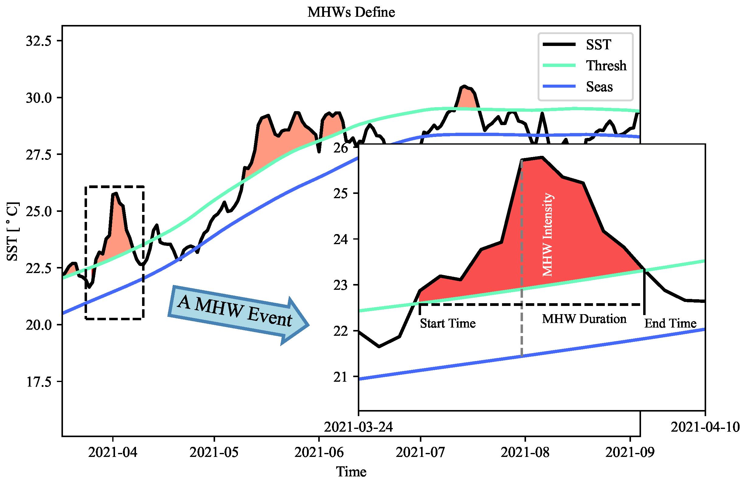
Figure 1.
The framework of using interpretive deep learning for marine heatwaves.
Figure 1.
The framework of using interpretive deep learning for marine heatwaves.
Figure 2.
The locations of the various stations taken in the coastal ocean areas of China.
Figure 2.
The locations of the various stations taken in the coastal ocean areas of China.
Figure 3.
This is an LSTM cell unit that includes a cell state vector , a hidden state vector , and the current input .
Figure 3.
This is an LSTM cell unit that includes a cell state vector , a hidden state vector , and the current input .
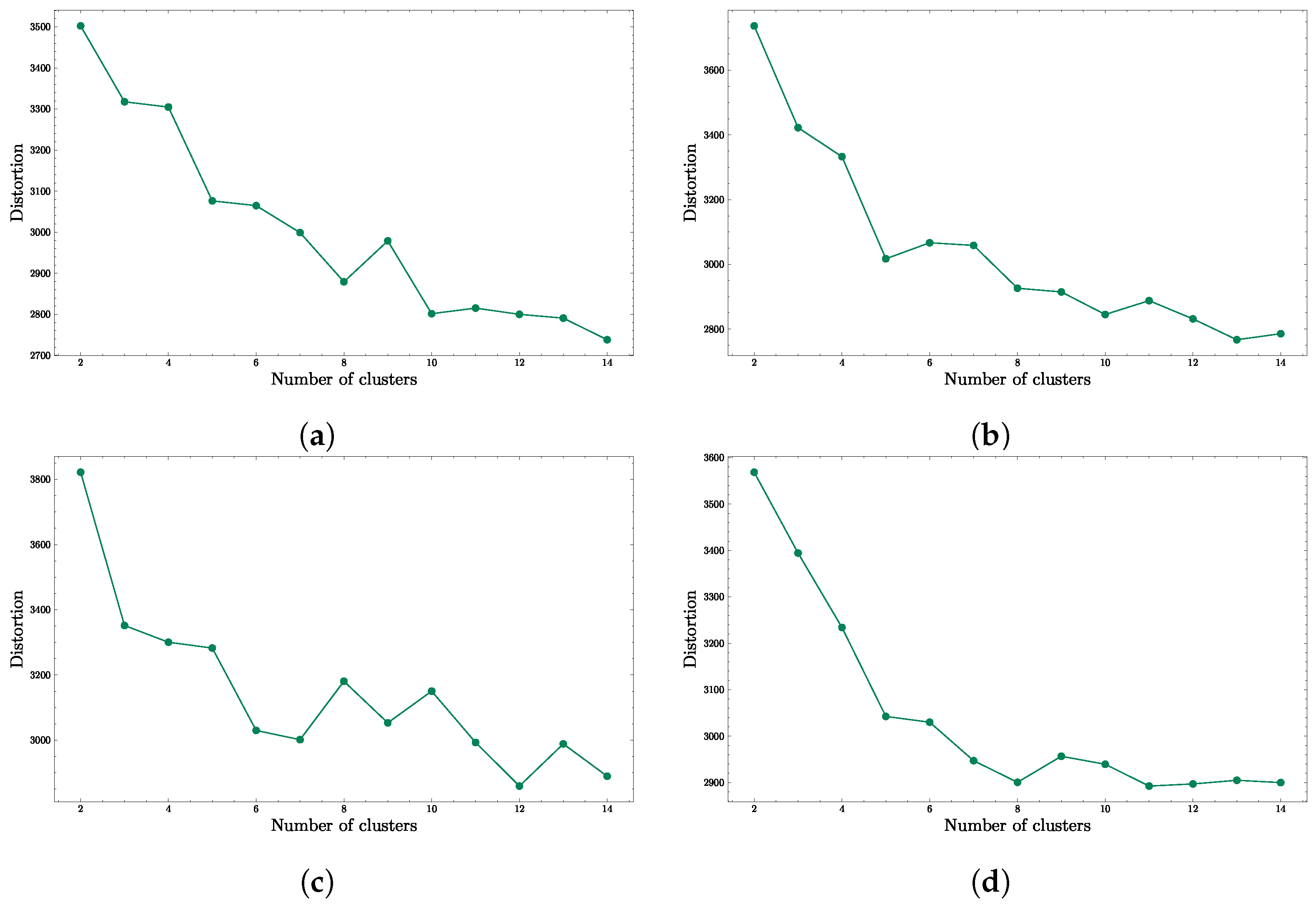
Figure 5.
The determination results of the elbow clustering number under different independent experiments. (a) presents the results with a random seed of 100 and a time step of 180. (b) displays the results with a random seed of 200 and a time step of 180. (c) shows the results with a random seed of 100 and a time step of 240. (d) depicts the results with a random seed of 200 and a time step of 240.
Figure 6.
The results under different cluster categories, where the first column represents the clustering results of sea surface pressure feature importance, and the second column represents the clustering results of 10m wind speed feature importance. Moreover, in each figure, the darkest curve represents the cluster center of each category.
Figure 7.
The number of events in different categories contained at different station.
Figure 7.
The number of events in different categories contained at different station.
Figure 8.
The number of each type of event in the sea areas of China.
Figure 8.
The number of each type of event in the sea areas of China.
Figure 9.
The marine heatwave event that occurred at BSG station on 7 August 2020, and its corresponding feature importance. The first and second row plots represent the historical data of different points in the 180 days before the marine heatwave event, with colors indicating the feature importance at different time points. The third row plot represents the predicted and observed sea surface temperature values. The fourth and fifth row plots represent the feature importance of pressure and 10 m wind speed, respectively.
Figure 10.
The marine heatwave event that occurred at DSN station on 12 August 1989, and its corresponding feature importance. The first and second row plots represent the historical data of different points in the 180 days before the marine heatwave event, with colors indicating the feature importance at different time points. The third row plot represents the predicted and observed sea surface temperature values. The fourth and fifth row plots represent the feature importance of pressure and 10 m wind speed, respectively.
Figure 11.
The marine heatwave event that occurred at NJI station on 3 June 1991, and its corresponding feature importance. The first and second row plots represent the historical data of different points in the 180 days before the marine heatwave event, with colors indicating the feature importance at different time points. The third row plot represents the predicted and observed sea surface temperature values. The fourth and fifth row plots represent the feature importance of pressure and 10 m wind speed, respectively.
Figure 12.
The marine heatwave event that occurred at ZFD station on 11 June 2004, and its corresponding feature importance. The first and second row plots represent the historical data of different points in the 180 days before the marine heatwave event, with colors indicating the feature importance at different time points. The third row plot represents the predicted and observed sea surface temperature values. The fourth and fifth row plots represent the feature importance of pressure and 10 m wind speed, respectively.
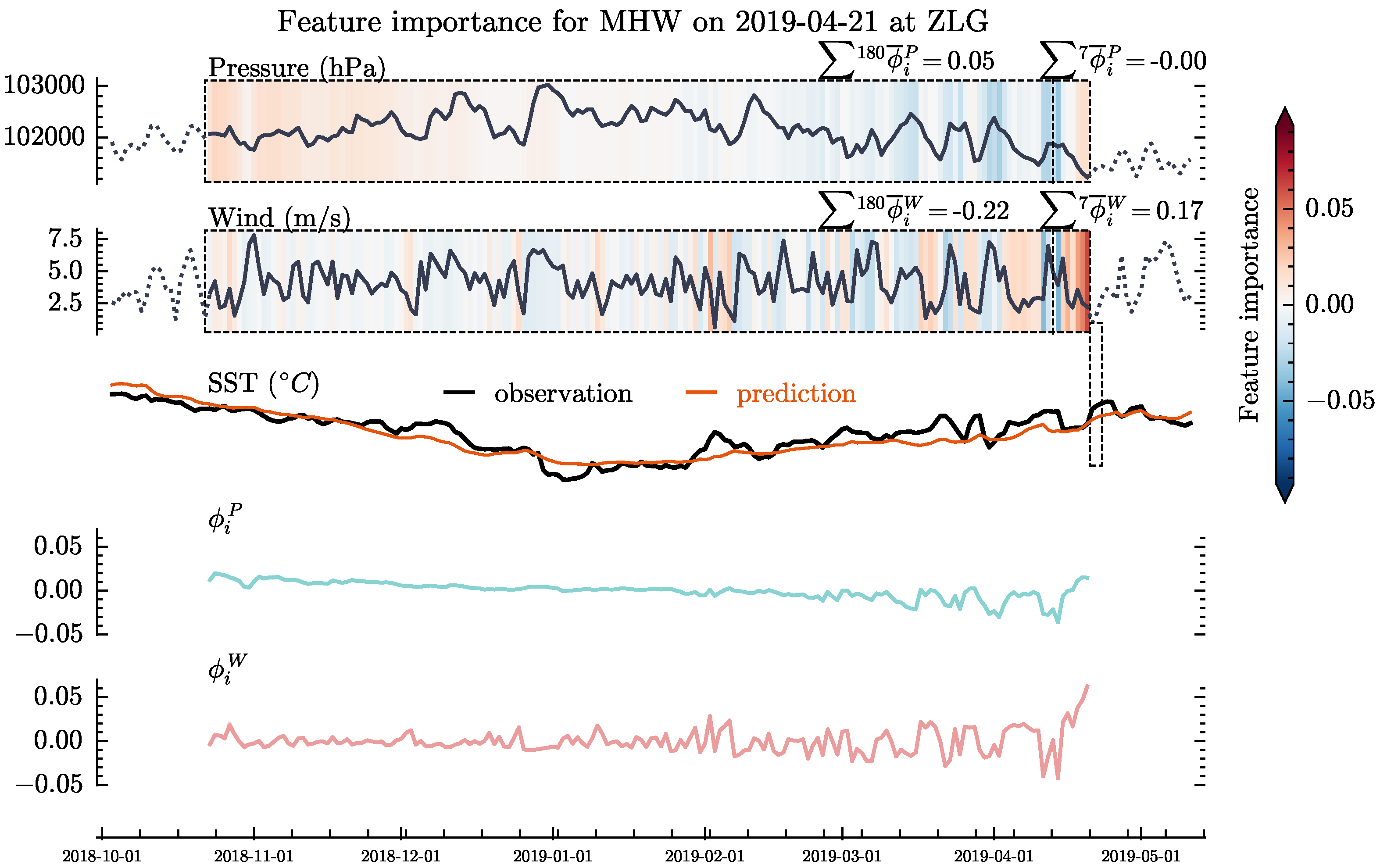
Figure 13.
The marine heatwave event that occurred at ZLG station on 21 Apirl 2019, and its corresponding feature importance. The first and second row plots represent the historical data of different points in the 180 days before the marine heatwave event, with colors indicating the feature importance at different time points. The third row plot represents the predicted and observed sea surface temperature values. The fourth and fifth row plots represent the feature importance of pressure and 10m wind speed, respectively.
Figure 14.
Performed AD analysis on the marine heatwave event that occurred at the NJI station on 3 June 1991.
Figure 14.
Performed AD analysis on the marine heatwave event that occurred at the NJI station on 3 June 1991.
Figure 15.
Performed AD analysis on the marine heatwave event that occurred at the NJI station on 21 April 2009.
Figure 15.
Performed AD analysis on the marine heatwave event that occurred at the NJI station on 21 April 2009.
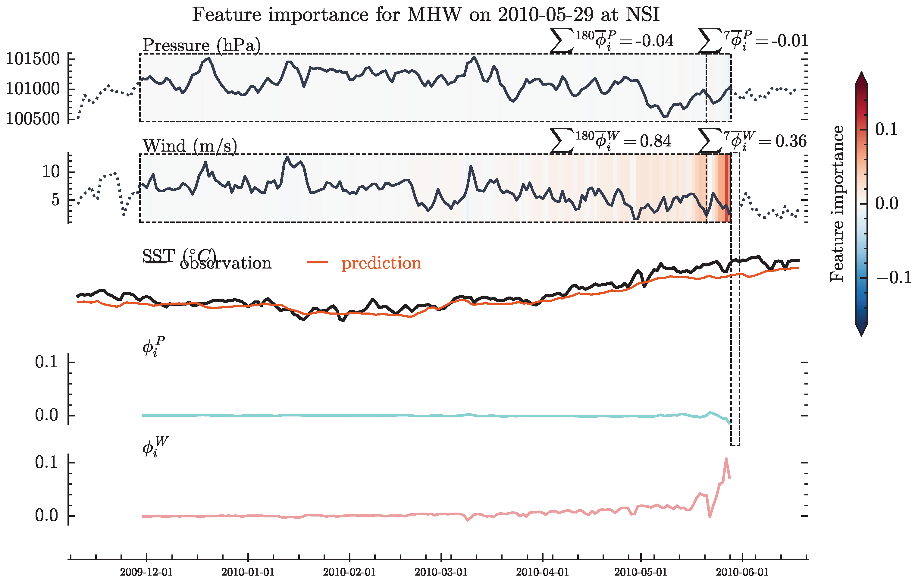
Figure 16.
The marine heatwave event that occurred at NSI station on 29 May 2010, and its corresponding feature importance. The first and second row plots represent the historical data of different points in the 180 days before the marine heatwave event, with colors indicating the feature importance at different time points. The third row plot represents the predicted and observed sea surface temperature values. The fourth and fifth row plots represent the feature importance of pressure and 10m wind speed, respectively.
Table 1.
The Observational and Reanalysis Data Sets Used in This Study.
Table 1.
The Observational and Reanalysis Data Sets Used in This Study.
Table 2.
The longitude and latitude information of the various stations taken in the coastal sea areas of China.
Table 2.
The longitude and latitude information of the various stations taken in the coastal sea areas of China.
| Station | Latitude | Longitude | Mean Pressure (Pa) | Mean Wind Speed (m/s) | Mean SST (C) |
|---|
| Xiao Chang Shan (XCS) | 39.2 N | 122.7 E | 101,588.068 | 4.883 | 13.023 |
| Lao Hu Tan (LHT) | 38.9 N | 121.7 E | 101,596.832 | 4.302 | 13.175 |
| Zhi Fu Dao (ZFD) | 37.6 N | 121.4 E | 101,612.341 | 3.554 | 13.637 |
| Lian Yun Gang (LYG) | 34.8 N | 119.4 E | 101,620.127 | 3.463 | 15.472 |
| Lv Si (LSI) | 32.1 N | 121.6 E | 101,578.760 | 3.635 | 16.509 |
| Sheng Shan (SSN) | 30.8 N | 122.8 E | 101,548.275 | 5.869 | 18.484 |
| Da Chen (DCN) | 28.5 N | 121.9 E | 101,501.948 | 5.988 | 19.446 |
| Dong Shan (DSN) | 23.8 N | 117.5 E | 101,296.689 | 4.523 | 22.230 |
| Nan Ji (NJI) | 27.5 N | 121.1 E | 101,474.890 | 6.058 | 20.281 |
| Bei Shuang (BSG) | 26.7 N | 120.3 E | 101,443.244 | 5.337 | 20.814 |
| Zhe Lang (ZLG) | 22.7 N | 115.6 E | 101,238.041 | 3.938 | 24.022 |
| Beibu Gulf (BBG) | 20.62 N | 109.37 E | 101,060.593 | 5.225 | 25.244 |
| Nansha Islands (NSI) | 10.62 N | 114.62 E | 100,924.856 | 6.104 | 28.399 |
Table 3.
Indicators characterizing marine heatwaves (MHWs). In the formula, j represents a specific day within a year, and denote the start and end of the climatological baseline period, respectively, and T is the daily Sea Surface Temperature (SST) for day d of year y. represents the 90th percentile, where pertains to the set . The term denotes the standard deviation, and the time period is defined from to , with the day j falling within the window .
| Index | Symbol or Formula | Unit |
|---|
| Climatology | | C |
| Threshold | | C |
| Start and end of MHWs | | days |
| Duration | | days |
| Intensity(max/mean/variance) | | C |
Table 4.
Perform four independent experiments at 13 stations, with the Mean Squared Error (MSE) and Root Mean Squared Error (RMSE) results for each experiment.
Table 4.
Perform four independent experiments at 13 stations, with the Mean Squared Error (MSE) and Root Mean Squared Error (RMSE) results for each experiment.
| Exp | Metric | Station |
|---|
| BBG | BSG | DCN | DSN | LHT | LSI | LYG | NJI | NSI | SSN | XCS | ZFD | ZLG |
|---|
| No. 1 | MSE | 0.082 | 0.053 | 0.046 | 0.060 | 0.037 | 0.042 | 0.039 | 0.053 | 0.229 | 0.038 | 0.034 | 0.034 | 0.075 |
| RMSE | 0.286 | 0.231 | 0.215 | 0.245 | 0.193 | 0.202 | 0.195 | 0.230 | 0.478 | 0.194 | 0.184 | 0.182 | 0.274 |
| No. 2 | MSE | 0.079 | 0.055 | 0.053 | 0.065 | 0.040 | 0.045 | 0.041 | 0.051 | 0.208 | 0.039 | 0.064 | 0.032 | 0.082 |
| RMSE | 0.281 | 0.233 | 0.229 | 0.254 | 0.197 | 0.206 | 0.199 | 0.226 | 0.456 | 0.197 | 0.248 | 0.178 | 0.287 |
| No. 3 | MSE | 0.073 | 0.047 | 0.056 | 0.061 | 0.038 | 0.034 | 0.051 | 0.054 | 0.233 | 0.048 | 0.038 | 0.051 | 0.083 |
| RMSE | 0.270 | 0.217 | 0.234 | 0.246 | 0.192 | 0.181 | 0.219 | 0.230 | 0.483 | 0.217 | 0.190 | 0.217 | 0.288 |
| No. 4 | MSE | 0.074 | 0.047 | 0.044 | 0.063 | 0.042 | 0.051 | 0.039 | 0.050 | 0.222 | 0.039 | 0.034 | 0.024 | 0.080 |
| RMSE | 0.271 | 0.217 | 0.209 | 0.250 | 0.201 | 0.222 | 0.191 | 0.224 | 0.471 | 0.198 | 0.182 | 0.155 | 0.283 |
Table 5.
The number of events under different cluster categories.
Table 5.
The number of events under different cluster categories.
| Clustering Categories | Num |
|---|
| Cluster 1 | 54 |
| Cluster 2 | 211 |
| Cluster 3 | 235 |
| Cluster 4 | 318 |
| Cluster 5 | 316 |
| Total | 1134 |
Table 6.
Comparing existing studies with the interpretable data-driven model shown in
Figure 1 of this article, the data used for the model in this article are reanalysis data. The five types of marine heatwave patterns in the table respectively correspond to Nos. 1~5 as identified in experiments.
Table 6.
Comparing existing studies with the interpretable data-driven model shown in
Figure 1 of this article, the data used for the model in this article are reanalysis data. The five types of marine heatwave patterns in the table respectively correspond to Nos. 1~5 as identified in experiments.
| Research | Data and Model | Pattern |
|---|
| Pattern 1 | Pattern 2 | Pattern 3 | Pattern 4 | Pattern 5 |
|---|
| Hu et al. [43] | Reanalysis Data and Numerical Model | | | | | ✔ |
| Yao and Wang [44] | Reanalysis Data and Numerical Model | ✔ | | ✔ | | |
| Qi and Cai [45] | Reanalysis Data and Numerical Model | | ✔ | | | |
| Wang et al. [46] | Reanalysis Data and Numerical Model | | | | ✔ | ✔ |


