Article

Doppler Factor in the Omega-k Algorithm for Pulsed and Continuous Wave Synthetic Aperture Radar Raw Data Processing

by
Jhohan Jancco-Chara
*,
Facundo Palomino-Quispe
,
Roger Jesus Coaquira-Castillo
,
Julio Cesar Herrera-Levano
and
Ruben Florez
LIECAR Laboratory, Universidad Nacional de San Antonio Abad del Cusco (UNSAAC), Cusco 08003, Peru
*
Author to whom correspondence should be addressed.
Appl. Sci. 2024, 14(1), 320; https://doi.org/10.3390/app14010320
Submission received: 20 October 2023 / Revised: 23 December 2023 / Accepted: 25 December 2023 / Published: 29 December 2023
(This article belongs to the Special Issue Computational Sensing and Imaging II)

Abstract

:
Synthetic aperture radar (SAR) raw data do not have a direct application; therefore, SAR raw signal processing algorithms are used to generate images that are used for various required applications. Currently, there are several algorithms focusing SAR raw data such as the range-Doppler algorithm, Chirp Scaling algorithm, and Omega-k algorithm, with these algorithms being the most used and traditional in SAR raw signal processing. The most prominent algorithm that operates in the frequency domain for focusing SAR raw data obtained by a synthetic aperture radar with large synthetic apertures is the Omega-k algorithm, which operates in the two-dimensional frequency domain; therefore, in this paper, we used the Omega-k algorithm to produce SAR images and modify the Omega-k algorithm by adding the Doppler factor to improve the accuracy of SAR raw data processing obtained by the continuous wave and pulsed frequency modulated linear frequency modulated radar system from the surfaces of interest. On the other hand, for the case of unmanned aerial vehicle-borne linear frequency modulated continuous wave (LFM-CW) SAR systems, we added motion compensation to the modified Omega-k algorithm. Finally, the testing and validation of the developed Omega-k algorithm used simulated and real SAR raw data for both pulsed synthetic aperture and continuous wave radars. The real SAR raw data used for the validation of the modified Omega-k algorithm were the raw data obtained by the micro advanced synthetic aperture radar (MicroASAR) system, which is an LFM-CW synthetic aperture radar installed on board an unmanned aerial system and the raw data obtained by European remote sensing (ERS-2) satellite with a synthetic aperture radar installed.

1. Introduction

The synthetic aperture radar has applications in remote observation of the Earth’s surface, forest monitoring [1], agriculture [2], damage detection in earthquakes [3], maritime surveillance [4], cartography, topography [5], and the generation of three-dimensional models of the surface of interest [6]. The synthetic aperture radar system can be installed on board space vehicles such as satellites, aerial vehicles such as UAVs (unmanned aerial vehicles) and airplanes, and ground vehicles such as automobiles automobilesar. Synthetic aperture radars transmit a chirp signal with linear frequency modulation through pulses; that is, they are pulsed synthetic aperture radars. Furthermore, it is not necessary to add the word pulsed because it is understood. Continuous waves with linear frequency modulation synthetic aperture radars transmit a chirp signal continuously; these radars are economically low cost compared with the SAR system [7].
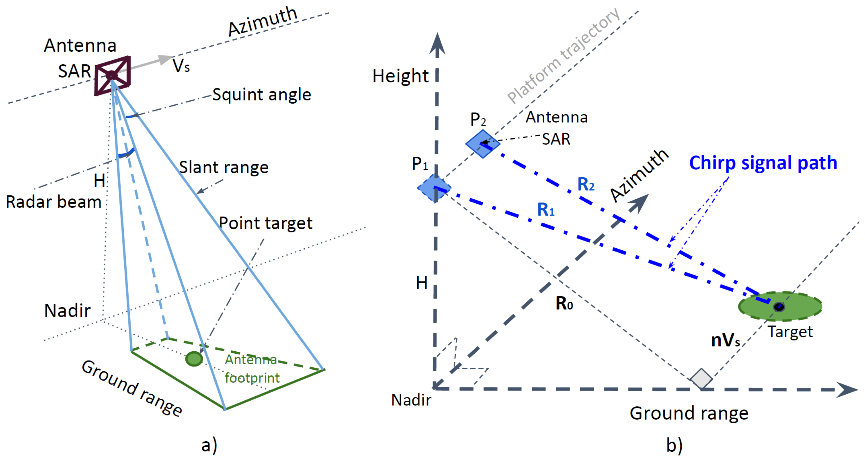
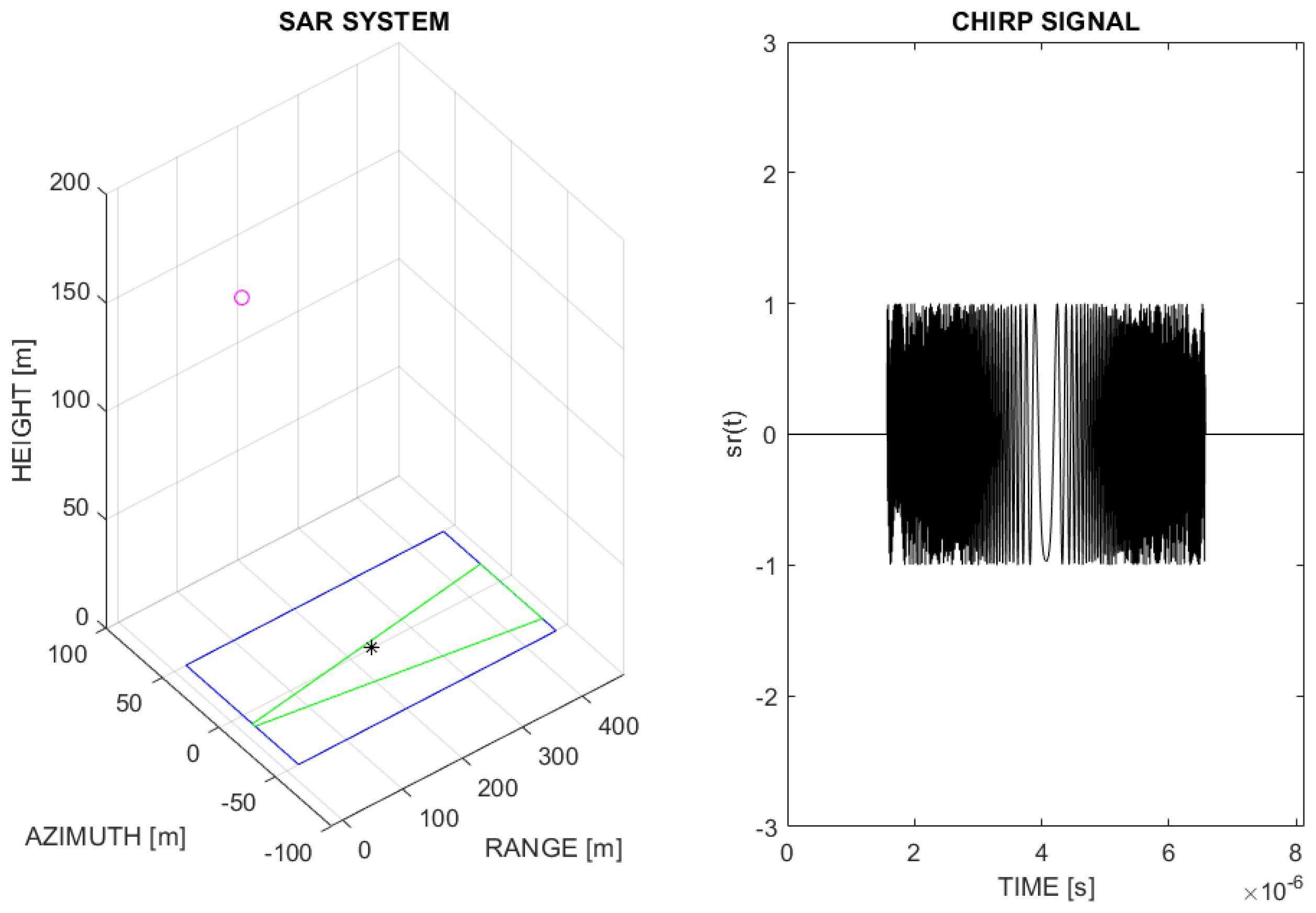
The operation of a synthetic aperture radar consists of the transmission of chirp signals and the subsequent reception of said chirp signals backscattered over a surface of interest. The platform of a synthetic aperture radar (SAR) system must move in a straight line with a constant speed to simulate a gigantic antenna using aperture synthesis. The reception of backscattered signals is carried out using an antenna [8]; these backscattered signals pass through the SAR system, which conditions them appropriately to generate SAR raw data.
SAR raw data are a matrix of raw signals [
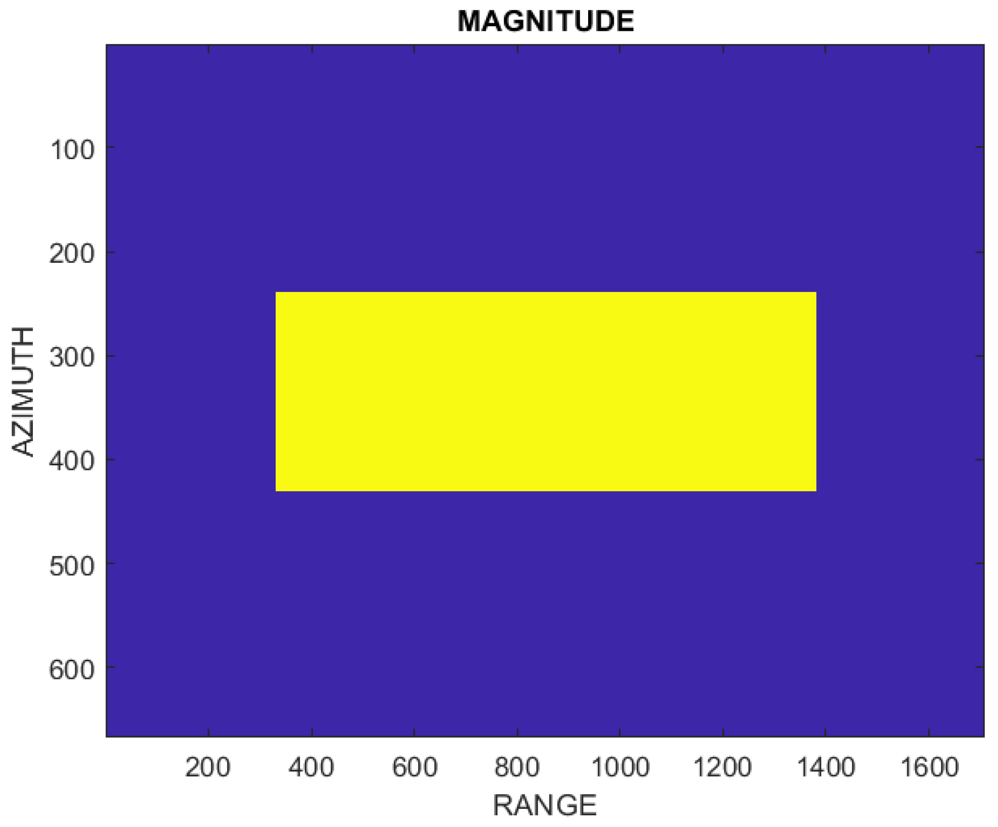
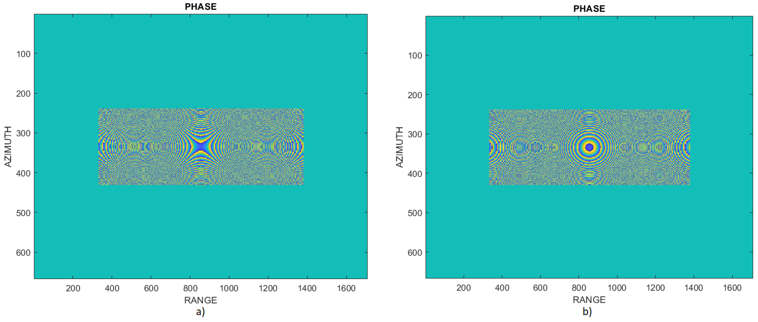
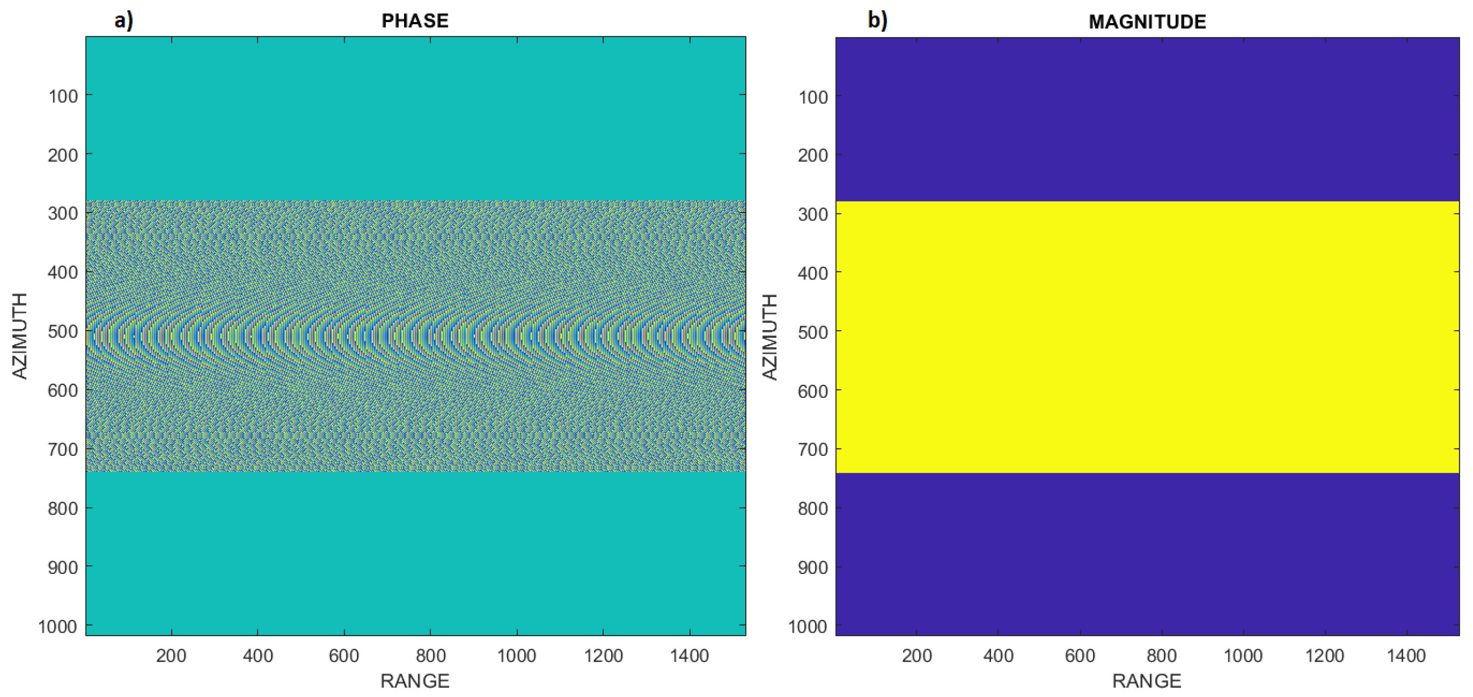
9] that are sampled using a slow time frequency in azimuth and a fast time frequency in range; the raw signal matrix contains electromagnetic information about the reflectivity of the surfaces of interest. On the other hand, SAR raw data elements are generally complex values; therefore, the amplitude of the complex values represents the intensity of the electromagnetic signal and the phase of that value contains distance, geometry, and surface feature information. SAR raw data have no direct applications because the desired results cannot be interpreted or described, so processing algorithms are used to generate SAR images where the surface of interest can be observed.
The range-Doppler algorithm [10], Chirp Scaling algorithm [11], and Omega-k algorithm [12] operate in the frequency domain and are the most widely used algorithms in synthetic aperture radar digital signal processing to generate SAR images. Time-domain focusing algorithms such as the backprojection algorithm [13] generate better quality SAR images compared with focusing algorithms operating in the frequency domain [14]; however, the advantage of frequency-domain focusing algorithms is that their computational cost is lower than that of the time-domain focusing algorithms [12,14]; therefore, frequency-domain focusing algorithms can be further improved. On the other hand, when the speed of the SAR platform is high or close to supersonic, hypersonic, and relativistic speeds, the Doppler factor is of the utmost importance. In recent research, the Doppler factor was only added in focusing algorithms for linear frequency modulated continuous wave (LFM-CW) SAR radars, obtaining good results [15]; however, the Doppler factor was not added in focusing algorithms for SAR (pulsed) radars installed on board a space platform and it is not known how the Doppler factor affects the SAR imaging approach. Therefore, in this paper, the Omega-k algorithm was chosen because it has a better performance than the Chirp scaling algorithm and the range-Doppler algorithm at large synthetic apertures [12,16], as well as to evaluate whether the Doppler factor has positive or negative effects on SAR raw signal processing.
In [17], the precise version of the Omega-k algorithm was developed for LFM-CW SAR radars, because this Omega-k algorithm only worked for pulsed SAR radars; as a result, a modified Omega-k algorithm for continuous wave radars was obtained, generating a good LFM-CW SAR image quality by distinguishing surfaces better than the range-Doppler algorithm; therefore, in this paper, we modify the Omega-k algorithm by adding motion compensation and Doppler factor for LFM-CW SAR radars to improve the focusing of the SAR images. Then, we present the structure of this paper and, in Section 1, we briefly describe a synthetic aperture radar, as well as its applications, SAR raw data structure, SAR raw signal processing algorithms, and problems. In 
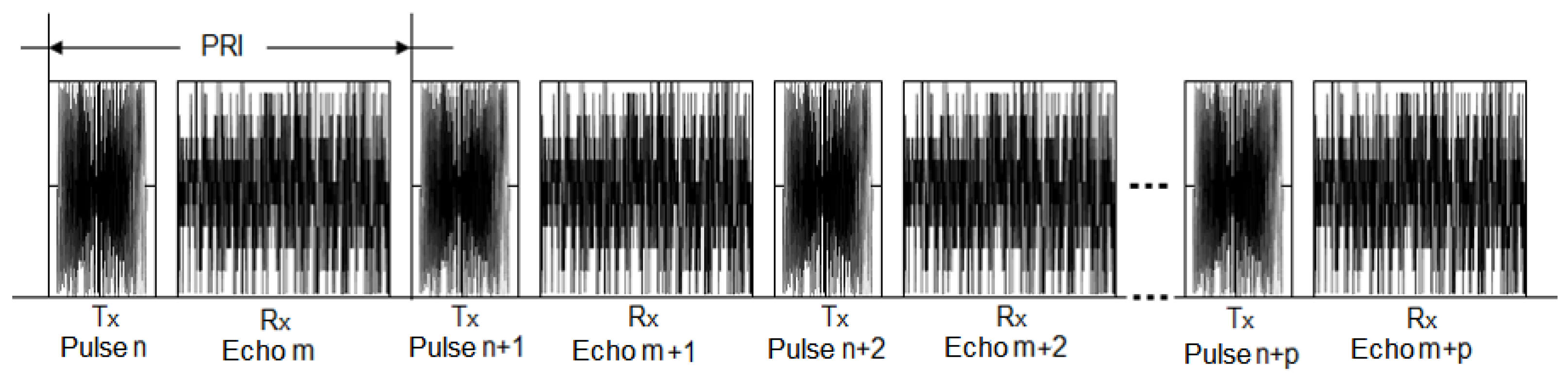
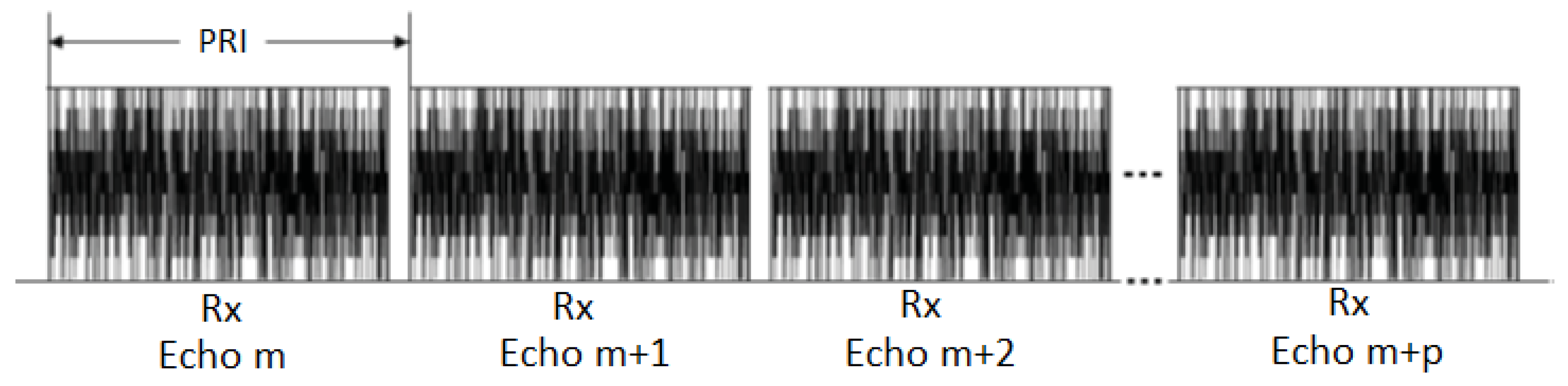
Section 2, we explain the SAR geometry, through a demonstration of the mathematical equation of the SAR raw data and the structure of continuous wave and pulsed SAR raw data. Then, in 
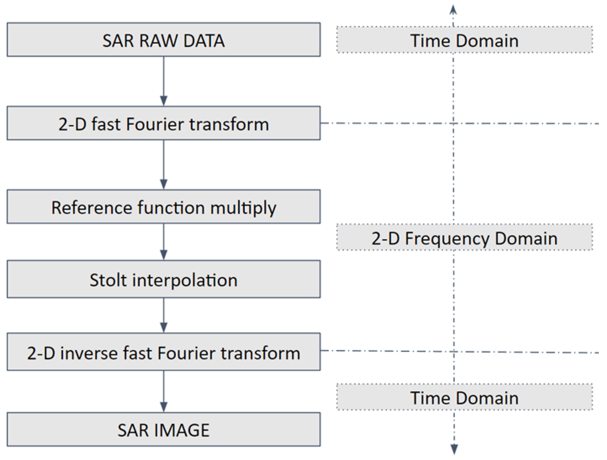
Section 3, we transform the SAR raw data from the time domain to the two-dimensional frequency domain. In Section 4, we develop SAR raw signal processing using the Omega-k algorithm for continuous wave and pulsed SAR radars. Then, in Section 5, the results are shown, that is, testing the Omega-k algorithm using simulated and real SAR raw data. Finally, Section 6 shows the conclusions and recommendations.

2. Syntethic Aperture Radar

A synthetic aperture radar (SAR) is a pulsed radar installed on board a space, air, or ground platform. It transmits chirp signals or electromagnetic waves with linear frequency modulation, obtaining a raw or unprocessed signal from the surface of interest through antennas, demodulators, filters, analog-to-digital converters, that is, through the signal conditioning system.

2.1. SAR Geometry

In Figure 1a, the SAR geometry is observed, which operates in stripmap mode and is a monostatic radar, where the magenta quadrilateral represents the SAR antenna, the green quadrilateral represents the SAR antenna footprint, the circle with a green background represents the target, and the SAR system movement direction is called azimuth and the chirp signal transmission direction is called the slant range. On the other hand, the Nadir point is also observed, where the Doppler effect is minimal; in addition, the squint angle, radar beam, and H SAR platform height are apparent.
In Figure 1b, the radar system moves from point P 1 to point P 2 in the azimuth direction to capture signals backscattered from the surface of interest through the SAR antenna; therefore, the blue lines represent the transmitted signal path (slant range R 1 ) and the backscattered chirp signal (slant range R 2 ), and this occurs at time Δ t . On the other hand, Equations (3) and (4) [16] are obtained from Figure 1b.
R 1 = R n
R 2 = R n + Δ t
R n = R 0 2 + V s n 2
R n + Δ t = R 0 2 + V s n + Δ t 2
where R 1 and R 2 are the slant range, Δ t is the time delay in acquiring backscattered signals from the surface of interest, n is the time in azimuth, and V s is the SAR platform speed; therefore, the time delay is as follows:
Δ t = R 1 + R 2 c
In Equation (5), we have the speed of light c, then replacing Equations (1) and (2) into Equation (5), we have the time delay Δ t .
Δ t = R n + R n + Δ t c
It is known that α = c 2 c 2     V s 2 is the Doppler factor [15,18]. Then, using Equations (3), (4) and (6), [14] the time delay Δ t is solved, therefore, the time delay Δ t of the chirp signal traveling through the paths of R 1 and R 2 is shown in Equation (7) [18].
Δ t = 2 α R ( n ) c + V s c 2 n

2.2. SAR Raw Signal Modeling

In Figure 2, the equation of the chirp signal transmitted by the SAR system through its antenna at point P 1 is represented by Equation (8) [9,16], and the backscattered signal from the surface of interest is received at point P 2 , and is described by Equation (9) [16,19,20].
s t t = r e c t t t p e x p j π k r t 2
where the transmitted chirp signal is s t , chirp modulation rate is k r , pulse duration is t p , and chirp signal received by the SAR antenna is s r which has a time delay Δ t .
s r t = r e c t t Δ t t p e x p j π k r t Δ t 2
Digital signal processing of synthetic aperture radar is achieved in phase and the amplitude can be neglected, as seen below, by expressing it with cosines.
s r t c o s 2 π f 0 t Δ t + π k r t Δ t 2
Then, Equation (10) can be expressed in another way, as shown in Equation (11), where ( t ) = 2 π f 0 Δ t + π k r t Δ t 2 is the backscattered signal phase and f 0 is the center frequency of the chirp signal.
s r t = c o s ( 2 π f 0 t + ( t ) )
Figure 2 shows the received signal modeling by the SAR antenna based on [16,19,20,21]. Where the received signal is multiplied by s r 1 t and s r 2 t , respectively, passing the resulting signal through the low-pass filter, eliminating the carrier signal, and then these signals are digitized obtaining the SAR raw signal s a t , which is determined mathematically in the following way for both the real and imaginary channels.
s r 1 t = s r t c o s 2 π f 0 t , s r 1 t = 1 2 c o s ( t ) + 1 2 c o s 4 π f 0 t + ( t )
s r 2 t = s r t s i n 2 π f 0 t , s r 2 t = 1 2 s i n ( t ) 1 2 s i n 4 π f 0 t + ( t )
Unwanted signals must be removed; therefore, the signal 1 2 s i n 4 π f 0 t + ( t ) is removed using a low-pass filter whose frequency spectrum is shown in Figure 3. Then, the filtered signals or resulting signals are shown in Equations (14) and (15) for both the real and imaginary channels, respectively.
s r r t = 1 2 c o s ( t )
s r i t = 1 2 s i n ( t )
s a t = 1 2 c o s ( t ) + 1 j s i n ( t )
Equation (16) can be expressed exponentially using Euler’s relation as follows: 1 2 e x p 1 j ( t ) . Then, returning the rectangular function to Equation (16), the SAR raw signal is obtained as shown in Equation (17), similar to that in [16,19,20]. Where the phase e x p 1 j ( t ) is used for generating SAR images through digital signal processing.
s a t r e c t t Δ t t p e x p 1 j ( t )
Figure 1 shows that the chirp signal is transmitted at point P 1 , and said chirp signal with a time delay is received by the antenna at point P 2 . In pulsed SAR systems, an antenna is used for the transmission and reception of chirp signals, as shown in Figure 4 where the pulse repetition interval P R I is the signal period in Figure 4, and in a system pulse, n is transmitted and m is received, then pulse n + 1 is transmitted and receives m + 1 , and so on.

2.3. LFM-CW SAR Raw Signal Modeling

Modeling synthetic aperture radar signals with continuous wave linear frequency modulation is similar to the case of a pulsed SAR system; however, one way to quickly obtain the SAR signal is by multiplying the transmitted signal by the conjugate of the backscattered signal, as described in Equation (20), taking into account that s t c t is the signal transmitted by the LFM-CW SAR system and the backscattered signal received by the antennas of said system is s r c t [14,19,22].
s t c t = e x p j 2 π f 0 t + π k r t 2
s r c t = e x p j 2 π f 0 t Δ t + π k r t Δ t 2
The equation of the SAR raw signal with continuous wave linear frequency modulation is shown in Equation (21), similar to that in [14,19,22]. This equation is used in SAR digital signal processing to focus images.
s d c t = s t c t s r c * t
s d c t = e x p j 2 π f 0 Δ t + 2 π k r t Δ t π k r Δ t 2
In an LFM-CW SAR system, two antennas are used, one to transmit T x and the other to receive R x chirp signals, whose transmitted signal and the backscattered signal are shown in Figure 5. On the other hand, the LFM-CW SAR systems can use two or more transmitting and receiving antennas, and this depends on the application. Figure 6 shows the sampling of the backscattered signal by the slow time frequency also called pulse repetition frequency ( P R F = 1 / P R I ) .

2.4. SAR Raw Data

SAR raw data are an array of chirp signals (pulses of electromagnetic waves) backscattered from the surfaces of interest. Figure 7 shows the general structure of SAR raw data for pulsed and continuous SAR radars, and SAR raw data have no direct application and cannot distinguish targets or surfaces of interest; therefore, SAR images are generated by focusing algorithms.
The SAR raw data in Figure 7 are sampled in the azimuth direction using the slow time sampling frequency or pulse repetition frequency ( P R F = 1 / P R I ) , the inverse of the pulse repetition frequency ( P R F ) is called the pulse repetition interval ( P R I ) ; the data are also sampled in the range direction using the fast time sampling frequency or sampling frequency ( f s ) .

3. Two-Dimensional Frequency Domain

Focusing algorithms that operate in the frequency domain have a lower computational cost than focusing algorithms that operate in the time domain; according to the literature the Omega-k algorithm has a better focusing quality than the Chirp Scaling algorithm and the range-Doppler algorithm for large synthetic apertures [12], so the Omega-k algorithm will be developed by adding parameters such as Doppler factor [15] for pulsed and continuous-wave SAR radars.

3.1. SAR Raw Signal Spectrum

The Omega-k algorithm works in the two-dimensional frequency domain; therefore, Fourier transform is applied in the azimuth and range direction to the SAR raw signal. On the other hand, for SAR signal processing, Equation (17) will be used, and rewriting said equation results in Equation (22), similar to that in [16,19,23,24].
s a t = r e c t t Δ t t p e x p 1 j 2 π f 0 Δ t + π k r t Δ t 2
In Equation (22), digital signal processing is mainly conducted in phase; therefore, the range Fourier transform is applied.
S A f t = s a t e x p j 2 π f t t d t ; ψ t = 2 π f 0 Δ t + π k r t Δ t 2 2 π f t t
where ψ t is the integrand phase and f t is the fast-time frequency. Then, the derivative is applied to ψ t and is set equal to zero because it is a stationary signal, then t is solved; mathematically speaking d ψ t d t = 0 , solving for t, we obtain the following:
t = Δ t + f t k r
Replacing Equation (24) in Equation phase (23), [16,20,24] or ψ t , obtains the following phase:
ψ f t = 2 π f 0 + f t Δ t π f t 2 k r
The development of digital signal processing is conducted in the SAR raw signal phase, so for now, we only considered the phase. Then, using Equations (23) and (24), the following result was obtained.
S A f t = e x p j ψ f t
Then, using the signal of Equation (26), which is in the range-Doppler domain, we transform the signal to the two-dimensional frequency domain by applying the azimuth Fourier transform.
S A f t , f n = S A f t e x p j 2 π f n n d t ; ψ f t , n = 2 π f 0 + f t Δ t π f t 2 k r 2 π f n n
where ψ f t , n is the integrand phase of Equation (27), f n is the slow time frequency, and Δ t = 2 α R ( n ) c + V s c 2 n is the delay time; then, as it is a stationary signal, d ψ f t , n d t = 0 . The value of n is shown in Equation (28).
n = R 0 f n c 2 α V s f 0 + f t + V s c V s 1 f n c 2 α V s f 0 + f t + V s c 2
Then, we replace n in Equation (27), finally obtaining a phase in the two-dimensional frequency domain and, consequently, the raw signal in the two-dimensional domain, which is shown in Equation (29).
S A f t , f n = e x p j ψ f t , f n
where:
ψ f t , f n = 4 π α R 0 c f 0 + f t 2 f n c 2 α V s + V s c f 0 + f t 2 π f t 2 k r

3.2. LFM-CW SAR Raw Signal Spectrum

The LFM-CW SAR raw signal in the time domain was obtained by the linear frequency modulated continuous wave (LFM-CW) synthetic aperture radar (SAR) system; then, we converted said signal to the two-dimensional frequency domain. Therefore, the range Fourier transform was first applied to Equation (21), as shown in Equation (31).
S D C f t = s d c t e x p j 2 π f t t d t
The range Fourier transform was applied, making f 0 f 0 + f t [16,17]; thus, we obtained Equation (32), which is in the range-Doppler domain.
S D C f t = I f t e x p j 2 π f 0 + f t Δ t π k r Δ t 2
where I f r is the s i n c amplitude of the signal; however, the processing was conducted in phase, so this amplitude was not taken into account. The residual video phase was removed; that is, the π k r Δ t 2 phase was removed, which is known as the residual phase removal.
S D C f t = e x p j 2 π f 0 + f t Δ t
The azimuth Fourier transform was applied to convert the signal in Equation (33), which was in the range-Doppler domain to the two-dimensional frequency domain.
S D C f t , f n = S D C f t e x p j 2 π f n n d n
Then, the integrand phase of Equation (34) is shown in Equation (35), and the derivative was applied and set equal to zero because it was a stationary signal. newpage
ω f t , n = 2 π f 0 + f t Δ t 2 π f n n ; d ω f t , n d n = 0
After applying the derivative, we had n and substituted it into phase θ f t , n , obtaining the phase shown in expression (36).
n = R 0 f n c 2 α V s f 0 + f t V s c V s 1 f n c 2 α V s f 0 + f t V s c 2
Finally, for SAR raw signals collected by linear frequency modulation continuous wave radars, we use Equation (37), which is in the two-dimensional frequency domain.
S D C f t , f n = e x p j ω f n , f t
where
ω ( f n , f t ) = 4 π α R 0 c f 0 + f t 2 c f n 2 α V s V s c f 0 + f t 2

4. SAR Raw Signal Processing

In this paper, the SAR raw signal processing is performed in the two-dimensional frequency domain using the Omega-k algorithm, which consists of general focusing and differential focusing.

4.1. Omega-k Algorithm for SAR System

The SAR raw data processing for a pulsed radar was implemented using Figure 8 based on [16]; therefore, the Omega-k algorithm was modified by adding the Doppler factor, so it will be developed in detail.

4.1.1. 2D Fast Fourier Transform

Firstly, the SAR raw data are a matrix of raw signals sampled over slow time in azimuth and fast time in the range frequencies. On the other hand, the Omega-k algorithm operates in the two-dimensional frequency domain; therefore, two-dimensional Fourier transform, that is, in range and azimuth, is applied to convert the data from the time domain to the frequency domain in the range and azimuth directions.

4.1.2. Reference Function Multiply

The SAR raw data in the two-dimensional frequency domain are shown in Equation (29); therefore, we implemented general focus, which consists of multiplying the data by the reference function is shown in Equation (39).
H r e f f t , f n = e x p j ψ r e f f t , f n
where
ψ r e f f t , f n = 4 π α R r e f c f 0 + f t 2 f n c 2 α V s + V s c f 0 + f t 2 π f t 2 k r
Then, the data are multiplied in the two-dimensional frequency domain S A f t , f n with the reference function H r e f f t , f n in the following way.
S A f t , f n H r e f f t , f n = e x p 1 j ψ f t , f n ψ r e f f t , f n
Then, the signal result phase S A f t , f n is as follows:
ψ R F M f t , f n = 4 π α R 0 R r e f c f 0 + f t 2 f n c 2 α V s + V s c f 0 + f t 2

4.1.3. Stolt Interpolation

Stolt interpolation consists of the exchange of f t for f t , similar to that in [16,22], that is, it is the exchange of frequencies, as shown in the following expression.
f 0 + f t 2 f n c 2 α V s + V s c f 0 + f t 2 = f 0 + f t
Therefore, the phase equation of the SAR raw data compressed in the range and azimuth is shown in Equation (44) [12,16].
ψ R F M f t , f n 4 π α R 0 R r e f c f 0 + f t
where ψ R F M f t , f n is the phase of the data compressed in the azimuth and range in the two-dimensional frequency domain.

4.1.4. 2D Inverse Fast Fourier Transform

We used the two-dimensional inverse Fourier transform to go from the two-dimensional frequency domain to the time domain, thus generating a SAR image.

4.2. Omega-k Algorithm for LFM-CW SAR System

In this paper, the raw signal processing of a continuous wave linear frequency modulated synthetic aperture radar is based on the Omega-k algorithm; therefore, we modified the omega-k algorithm as shown in Figure 9, and each one of the blocks is described in the following sections.

4.2.1. Fast Fourier Transform in Range

The range Fourier transform is applied to the LFM-CW SAR raw data, and the fast Fourier transform is used to convert the data from the time domain to the range-Doppler domain, because it is an algorithm to calculate the Fourier transform.

4.2.2. Residual Video Phase Removal

Then, we proceeded to eliminate the residual video phase by multiplying Equation (32) by e x p j π k r Δ t 2 to eliminate said unwanted phase. This phase should be eliminated because it negatively affects image quality due to its negative impact on distance measurement applications, errors in velocity measurement, and causing blurring in the LFM-CW SAR image. Equation (45) is used to remove the residual phase of the video.
H R V P = e x p j π k r Δ t 2

4.2.3. Motion Compensation 1

If the range R n R n + Δ R n , then motion compensation is applied, which consists of multiplying the data by H m c 1 or equation (46) to remove the unwanted phase.
H m c 1 = e x p j 4 π α Δ R n c f 0 + f t
where Δ R n is the distance variation or range variation, and it is dependent on the time in azimuth n.

4.2.4. Fast Fourier Transform in Azimuth

The azimuth Fourier transform is applied to the data using fast Fourier transform in azimuth, then the data are transformed to the two-dimensional frequency domain as shown in Equation (37).

4.2.5. Reference Function Multiply

The general focusing is implemented using referential slant range, which consists of multiplying the data in the two-dimensional frequency domain by a reference function, as shown in Equation (47).
H r e f f t , f n = e x p 1 j ω r e f f n , f t
where:
ω r e f f n , f t = 4 π α R r e f c f 0 + f t 2 c f n 2 α V s V s c f 0 + f t 2

4.2.6. Stolt Interpolation

Differential focusing or Stolt interpolation consists of exchanging f t for f t , which is normally carried out in the processing of pulsed SAR radars [16,22]. Equation (49) describes the stolt interpolation.
f 0 + f t 2 c f n 2 α V s V s c f 0 + f t 2 = f 0 + f t
Another way to perform Stolt interpolation is by performing a difference of quadratic factors [17], as shown in Equation (50). The compressed data phase in the range and azimuth in two-dimensional domain is shown in Equation (51) [12,16].
f t = f 0 + f t 2 c f n 2 α V s V s c f 0 + f t 2 f 0 2 c f n 2 α V s V s f 0 c 2
ω R F M f t , f n 4 π α R 0 R r e f c f 0 + f t

4.2.7. Inverse Fast Fourier Transform in Azimuth

The inverse fast Fourier transform (IFFT) is applied in the azimuth; however, the inverse transform is no longer applied in the range because it is not necessary, and it is enough to apply the Fourier transform in the range for the image quality to be acceptable.

4.2.8. Motion Compensation 2

Equation (52) [25] can be applied as an approximate motion compensation in the time domain; however, H m c 2 = t 4 can also be applied because the data are in the time domain.
H m c 2 = t 3
Finally, filters are applied to eliminate speckle noise, and the most common filter used is the multilook filter.

5. Results of Testing the Omega-k Algorithm

Testing of the algorithm is carried out using simulated and real SAR raw data, and doing the same for synthetic aperture radars with continuous wave linear frequency modulation.

5.1. Simulated SAR Raw Data

Figure 10 shows the simulation of the synthetic aperture radar geometry used to simulate SAR raw data with the main parameters of Table 1 and Equation (17). Additionally, Figure 10 shows a magenta circle located at a certain height that represents the SAR platform. On the other hand, the green triangle represents the antenna footprint that once contained the black asterisk, which is an isolated and isotropic white dot, and it generates a chirp signal. Otherwise, if the footprint does not contain the black asterisk, it does not generate a chirp signal.
Table 1 shows the initial parameters used to simulate a synthetic aperture radar that transmits a chirp signal or an electromagnetic pulse signal with a linear frequency modulation, as seen in Figure 10. This SAR system operates in the C band, for which the center frequency of the chirp signal is 5 GH z , and the bandwidth of 150 MH z determines the distance resolution.
Figure 11 shows the magnitude plot of the SAR raw data, because this data have elements that are complex values; therefore, Figure 12 shows the SAR raw data phase of an isolated and isotropic point target that serves to test the proposed Omega-k algorithm and test the approximate quality of the SAR images.
In Figure 12a, it is observed that the SAR raw data phase has the shape of a hyperbola and it indicates that the phase of the transmitted signal has a positive slope or is also known as Up-Chirp. On the other hand, in Figure 12b, the the SAR raw data phase have the shape of an ellipse, which indicates that the derivative of the phase of the transmitted signal has a negative slope and is known as Down-Chirp.
Figure 13 shows a SAR image of a point target located in the center of the image with the azimuth and range directions generated from the simulated SAR raw data shown in Figure 11.
The SAR image in Figure 13 has pixels that are complex values; therefore, the image shown in said figure is the magnitude of the SAR image demonstrating the correct operation of the modified Omega-k algorithm for the SAR system (pulsed), and simulating the SAR raw data using the proposed Omega-k algorithm is validated.
On the other hand, Table 2 shows the approximate values of the parameters of the SAR images of a point target by making a cut in the azimuth and range at the point or pixel of the maximum intensity of the SAR image shown in Figure 13. The quality parameters of the Omega-k algorithm are shown in Table 2, for which the values of the quality parameters are acceptable. These approximate parameters were calculated by simulating the antenna footprint with the parameters of Table 1 along the azimuth and a point target. These quality parameters vary depending on the dimensions of the antenna footprint and observed scene.

5.2. Real SAR Raw Data and Discussion

Figure 14a shows the magnitude of the actual SAR raw data acquired by the Active Microwave Instrument that is installed on the ERS-2 satellite. Figure 14b shows the SAR image obtained with the unmodified Omega-k algorithm, also called precise version algorithm; meanwhile, in Figure 14c, the SAR image obtained using the range-Doppler algorithm is observed. The focusing algorithm used by the ERS-2 system is the range-Doppler algorithm (SAR Training Processor v1.1). On the other hand, comparing Figure 14b,c it is observed that they are similar; however, some parts of the surface are better observed in the SAR image using the Omega-k algorithm.
The SAR raw data come from the surface of Lake Titicaca in Bolivia, a photograph of which is shown in Figure 15a [26] and the magnitude of SAR raw data is shown in Figure 15b [26]. These raw data were acquired by the European Remote Sensing satellite (ERS-2) through its active sensor, known as the synthetic aperture radar with pulsed linear frequency modulation (LFM), whose SAR system’s main parameters are shown in Table 3. then, the SAR image generated with the proposed Omega-k algorithm is shown in Figure 16, and it is observed that the SAR images of Figure 14c and Figure 16 are similar; furthermore, Figure 17 shows three samples obtained from Figure 14b,c and Figure 16, that is, images obtained with the Omega-k algorithm, range-Doppler algorithm, and the proposed Omega-k algorithm. A selected area with a blue outline is seen clearer and sharper in the SAR image obtained with the proposed Omega-k algorithm compared with the range-Doppler algorithm and similar to the Omega-k algorithm; therefore, the proposed Omega-k algorithm works correctly. On the other hand, it was also tested using other real SAR raw data captured by the ERS-2 satellite, and the result of the modified Omega-k algorithm focusing is shown in Figure 15c, where a SAR image of a part of Lake Titicaca located in South America is observed. One limitation is the lack of SAR raw data obtained in air or space vehicles with high speeds or hypersonic speeds, so it would be advisable to test this proposed Omega-k algorithm on such SAR raw data to more effectively evaluate its performance.

5.3. Simulated LFM-CW SAR Raw Data

In Figure 18, the LFM-CW SAR system is represented by the black rhombus at a certain height, which moves in the azimuth direction and the chirp signals are transmitted and received in the slant range direction. The antenna footprint of the LFM-CW SAR system is represented by the green triangle and the green asterisk represents the isolated and isotropic point target; the blue quadrilateral is the scene scanned with the radar.
On the other hand, Figure 18 shows blue chirp signals, this observed chirp signal s ( t ) is continuous, which is called a continuous wave linear frequency modulated chirp. The LFM-CW SAR system is used to generate a continuous wave chirp signal with linear frequency modulation shown in Figure 18 using the main parameters of Table 4 and Equation (21); the magnitude and phase of the LFM-CW SAR raw data is shown in Figure 19, which has range and azimuth directions, and in the magnitude of the SAR raw data a yellow rectangle is observed that has no meaning and has no direct application.
The LFM-CW SAR image in Figure 20 of an point target is obtained from the LFM-CW SAR raw data shown in Figure 19 using the modified Omega-k algorithm.
The quality parameters shown in Table 5 are approximate because they depend on the dimensions of the scene. These parameters are obtained using Table 4 and performing a cut in azimuth and range at the most intense point or pixel of the SAR image of a point target (isolated and isotropic). On the other hand, P S L R R , P S L R A , I S L R R , and I S L R A are the peak side lobe ratio (PSLR) and integrated side lobe ratio (ISLR) in the range and azimuth, respectively.

5.4. Real LFM-CW SAR Raw Data and Discussion

Real LFM-CW SAR raw data obtained by the micro advanced synthetic aperture radar (MicroASAR) with linear frequency modulated continuous wave (LFM-CW) on board an unmanned aerial vehicle are obtained from “microASAR [28] data courtesy of David G. Long at Brigham Young University [29]”. On the other hand, Figure 21 shows a comparison of SAR images obtained between the range-Doppler algorithm and Omega-k algorithm.
Finally, the proposed Omega-k algorithm was validated by comparing the SAR images of Figure 21 and Figure 22; it was observed that they were similar as the same MicroASAR raw data were used, for which the main parameters are shown in Table 6. In Figure 22, the SAR image has range and azimuth directions, and the noise was reduced compared with Figure 21b. Figure 23 shows that in the selected area, the noise was significantly reduced, demonstrating the effectiveness of the proposed Omega-k algorithm. The SAR image shown in Figure 22b was georectified according to the range and azimuth resolutions of the MicroASAR system using the SAR image in Figure 22a.
In the selected area of Figure 23, a clean and noise-free surface could be observed compared with the SAR image of Figure 22b; in addition, improvements were also observed in the regions A and B of the SAR image in Figure 23. In the SAR images observed in Figure 17a, Figure 22, and Figure 23, the black areas represent absorbing surfaces, water bodies with turbulence, and areas with dense vegetation because the absorption of the chirp signals and the backscattered signal captured by the radar antenna was weak or the chirp signal was simply lost. Bright parts of SAR images represented reflective or rough surfaces, metallic objects, calm bodies of water, and urban areas. The intensities of each pixel of the SAR image depend on the incidence angle, surface geometry, vegetation water stress, antenna, and SAR geometry.

6. Conclusions

The SAR and LFM-CW SAR raw signals were transformed by adding the Doppler factor using the two-dimensional Fourier transform from the time domain to the two-dimensional Fourier domain, then the Omega-k algorithm was modified by adding the Doppler factor for continuous and pulsed wave synthetic aperture radars.
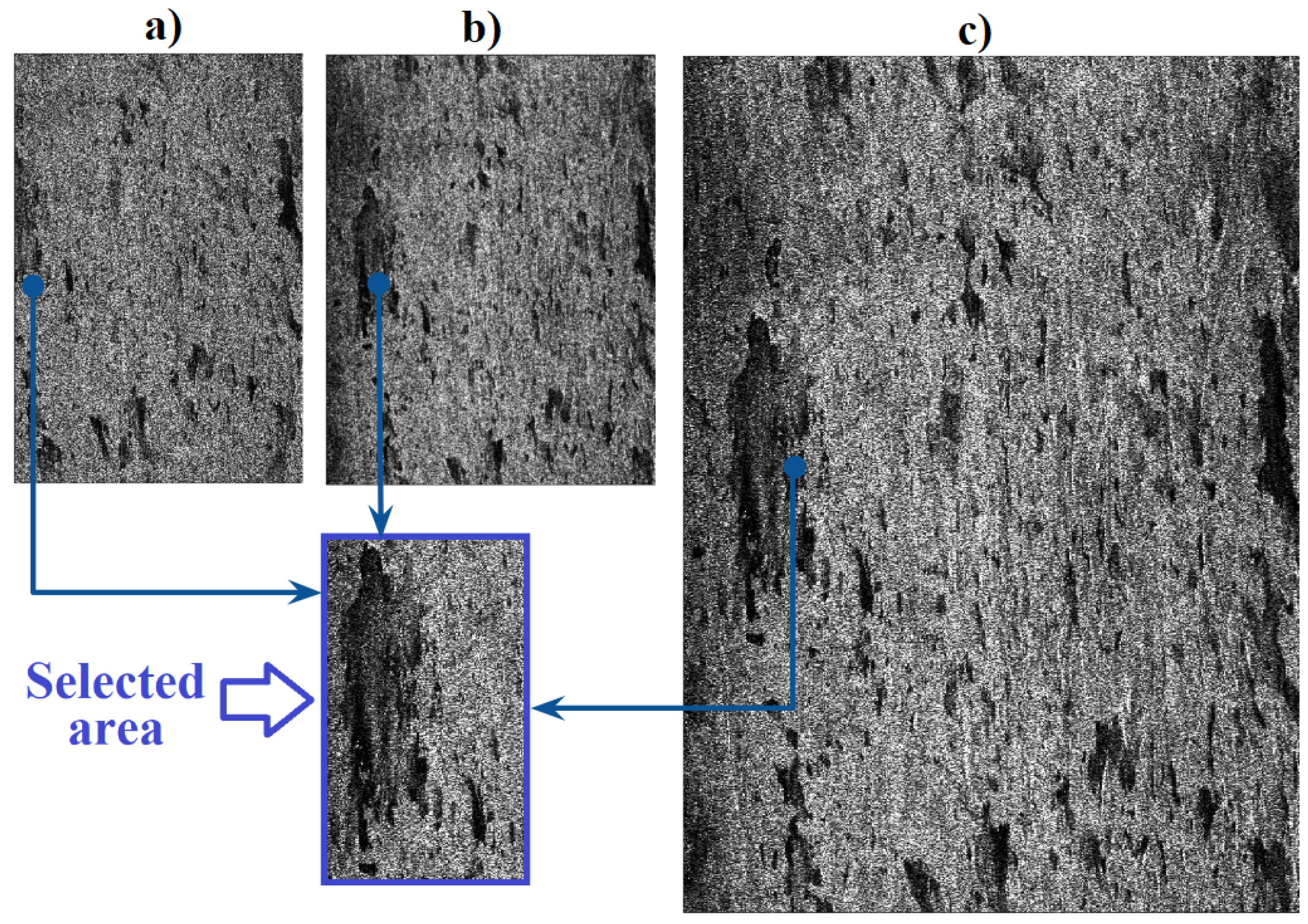
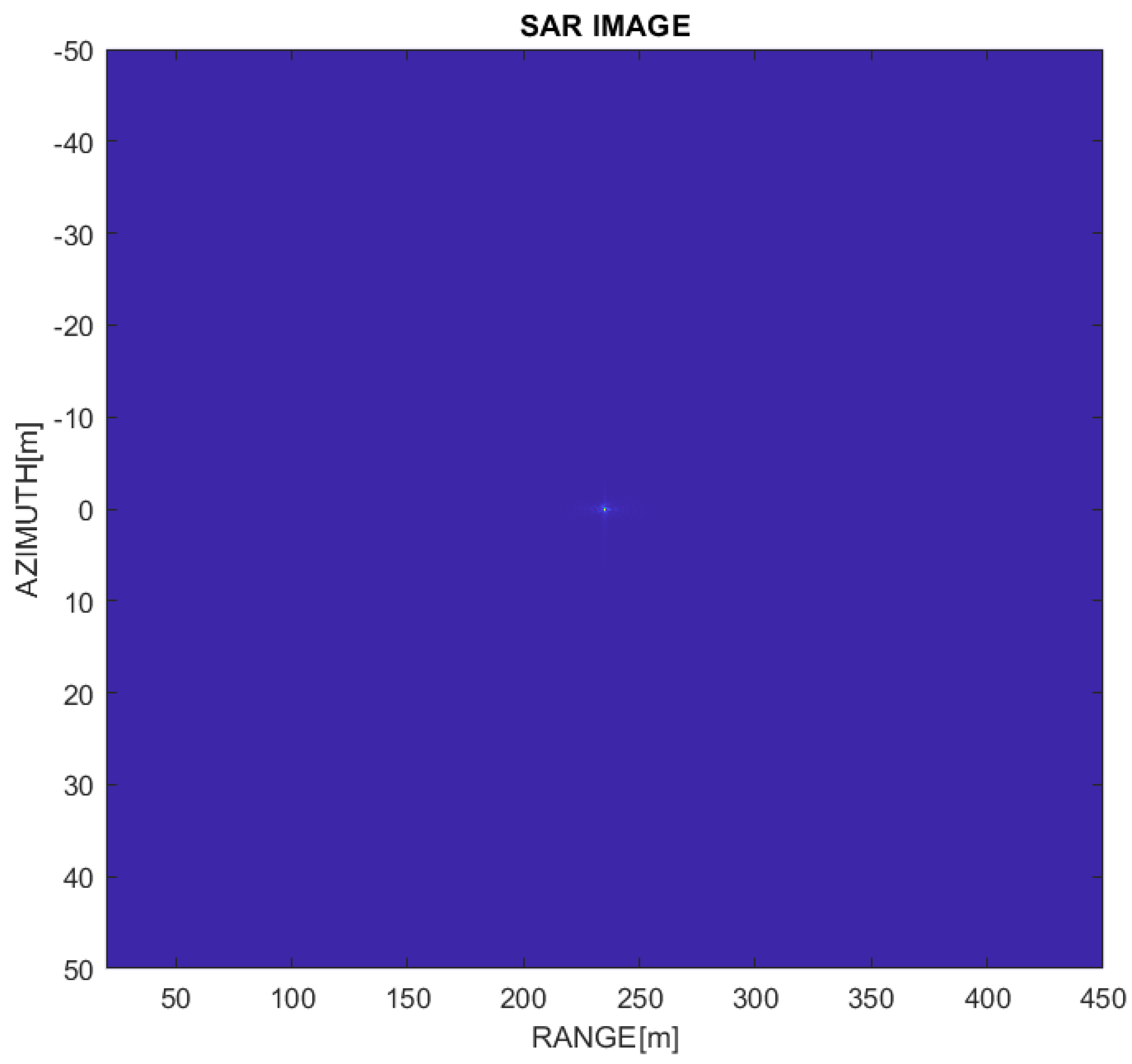
The modified Omega-k algorithm for SAR (pulsed) systems was validated using simulated SAR raw data from a point target; additionally, this modified Omega-k algorithm was validated with real SAR raw data that were obtained by the ERS-2 satellite through its SAR radar (pulsed). On the other hand, in the modified Omega-k algorithm for LFM-CW SAR systems, in addition to adding the Doppler factor, the SAR system aerial platform movement compensation was added. This Omega-k algorithm was validated with simulated SAR raw data and real SAR raw data obtained by the MicroASAR system that was installed on board an unmanned aerial vehicle.
SAR images generated by the modified Omega-k algorithm for continuous wave and pulsed SAR systems have pixels with complex values and have remote observation information of the surface of interest. These SAR images had range and azimuth directions, and these SAR images obtained with the range-Doppler algorithm and the modified Omega-k algorithm were compared, obtaining similar results and thus validating these proposed Omega-k algorithms. On the other hand, the modified Omega-k algorithm for the LFM-CW SAR system showed better results because of residual video phase elimination, and Doppler factor and motion compensation were added.
As a contribution to the scientific community, the Doppler factor was successfully added to the Omega-k algorithm for the pulsed SAR system, generating good quality SAR images. For future work, the application of the Omega-k algorithm is recommended with the addition of the Doppler factor for bistatic and circular synthetic aperture radars. It is also recommended that the effects of adding the Doppler factor in the range-Doppler algorithm and the chirp scaling algorithm in the approach of SAR raw data obtained on SAR platforms with high velocities are examined.

Author Contributions

Conceptualization, methodology, and algorithm, J.J.-C. and F.P.-Q.; validation and formal analysis, J.J.-C., F.P.-Q., R.J.C.-C. and R.F.; resources, F.P.-Q., R.J.C.-C. and J.C.H.-L.; data curation, J.J.-C.; writing—original draft preparation, J.J.-C. and F.P.-Q.; writing—review and editing, J.J.-C. and R.F.; supervision, R.F. and F.P.-Q.; project administration, F.P.-Q.; funding acquisition, F.P.-Q., R.J.C.-C. and J.C.H.-L. All authors have read and agreed to the published version of the manuscript.

Funding

This research received no external funding.

Institutional Review Board Statement

Not applicable.

Informed Consent Statement

Not applicable.

Data Availability Statement

The SAR raw data (Level Zero) used in this paper can be found in https://search.asf.alaska.edu or https://doi.org/10.5067/4KVOYM7NQ19L. More information about the LFM-CW SAR raw data can be found in https://api.semanticscholar.org/CorpusID:201822364.

Acknowledgments

The research was supported by the Institutional laboratory for research, entrepreneurship, and innovation in automatic control systems, automation, and robotics (LIECAR) at the University of San Antonio Abad del Cusco UNSAAC.

Conflicts of Interest

The authors declare no conflict of interest.

References

  1. Lang, M.W.; Kasischke, E.S. Using C-Band Synthetic Aperture Radar Data to Monitor Forested Wetland Hydrology in Maryland’s Coastal Plain, USA. IEEE Trans. Geosci. Remote Sens. 2008, 46, 535–546. [Google Scholar] [CrossRef]
  2. Sravani, N.; Mitravinda, R.; Kumar, P.R.; Neelima, N.; Sailaja, K.L. ACMapping: Agricultural Crop Mapping/Retrieval Using Synthetic Aperture Radar (SAR) Data. In Proceedings of the 2023 International Conference on Computer Communication and Informatics (ICCCI), Coimbatore, India, 23–25 January 2023; pp. 1–4. [Google Scholar] [CrossRef]
  3. Matsuoka, M.; Yamazaki, F. Application of the damage detection method using SAR intensity images to recent earthquakes. In Proceedings of the IEEE International Geoscience and Remote Sensing Symposium, Toronto, ON, Canada, 24–28 June 2002; Volume 4, pp. 2042–2044. [Google Scholar] [CrossRef]
  4. Pelich, R.; Longépé, N.; Mercier, G.; Hajduch, G.; Garello, R. AIS-Based Evaluation of Target Detectors and SAR Sensors Characteristics for Maritime Surveillance. IEEE J. Sel. Top. Appl. Earth Obs. Remote Sens. 2015, 8, 3892–3901. [Google Scholar] [CrossRef]
  5. Sui, X.; Liu, M.; Li, Y. Synthetic Aperture Radar Imaging of Abrupt Underwater Topography. In Proceedings of the 2020 IEEE 5th International Conference on Signal and Image Processing (ICSIP), Nanjing, China, 23–25 October 2020; pp. 479–482. [Google Scholar] [CrossRef]
  6. Hu, J.; Ding, X.L.; Zhang, L.; Sun, Q.; Li, Z.W.; Zhu, J.J.; Lu, Z. Estimation of 3-D Surface Displacement Based on InSAR and Deformation Modeling. IEEE Trans. Geosci. Remote Sens. 2017, 55, 2007–2016. [Google Scholar] [CrossRef]
  7. El-Darymli, K.; Moloney, C.; Gill, E.; McGuire, P.; Power, D. Design and implementation of a low-power synthetic aperture radar. In Proceedings of the 2014 IEEE Geoscience and Remote Sensing Symposium, Quebec City, QC, Canada, 13–18 July 2014; pp. 1089–1092. [Google Scholar] [CrossRef]
  8. Kothapudi, V.K.; Kumar, V. A 6-Port Two-Dimensional 3×3 Series-Fed Planar Array Antenna for Dual-Polarized X-Band Airborne Synthetic Aperture Radar Applications. IEEE Access 2018, 6, 12001–12007. [Google Scholar] [CrossRef]
  9. Khwaja, S. Fast Raw Data Generation of Realistic Environments for a SAR System Simulator. Ph.D. Thesis, Université Rennes 1, Lannion, France, 2009. [Google Scholar]
  10. Hughes, W.; Gault, K.; Princz, G. A comparison of the Range-Doppler and Chirp Scaling algorithms with reference to RADARSAT. In Proceedings of the 1996 International Geoscience and Remote Sensing Symposium (IGARSS ’96), Lincoln, NE, USA, 31 May 1996; Volume 2, pp. 1221–1223. [Google Scholar] [CrossRef]
  11. Raney, R.; Runge, H.; Bamler, R.; Cumming, I.; Wong, F. Precision SAR processing using chirp scaling. IEEE Trans. Geosci. Remote Sens. 1994, 32, 786–799. [Google Scholar] [CrossRef]
  12. Cumming, I.; Neo, Y.; Wong, F. Interpretations of the omega-K algorithm and comparisons with other algorithms. In Proceedings of the IGARSS 2003. 2003 IEEE International Geoscience and Remote Sensing Symposium (Proceedings IEEE Cat. No.03CH37477), Toulouse, France, 21–25 July 2003; Volume 3, pp. 1455–1458. [Google Scholar] [CrossRef]
  13. Israel Duersch, M. Backprojection for Synthetic Aperture Radar. Ph.D. Thesis, Brigham Young University, Provo, UT, USA, 2013. [Google Scholar]
  14. Zaugg, E.C. Generalized Image Formation for Pulsed and LFM-CW Synthetic Aperture RadarAperture Rada. Ph.D. Thesis, Brigham Young University, Provo, UT, USA, 2010. [Google Scholar]
  15. Wang, R.; Loffeld, O.; Nies, H.; Knedlik, S.; Hagelen, M.; Essen, H. Focus FMCW SAR Data Using the Wavenumber Domain Algorithm. IEEE Trans. Geosci. Remote Sens. 2010, 48, 2109–2118. [Google Scholar] [CrossRef]
  16. Cumming, I.G.; Wong, F.H.C. Digital Processing of Synthetic Aperture Radar Data: Algorithms and Implementation; Artech House: Norwood, MA, USA, 2005. [Google Scholar]
  17. Jancco Chara, J.; Palomino Quispe, F.; Coaquira Castillo, R.J.; Clemente-Arenas, M. Omega-k Algorithm Implementation for Linear Frequency Modulated-Continous Wave SAR Signal Processing. In Proceedings of the 2020 IEEE XXVII International Conference on Electronics, Electrical Engineering and Computing (INTERCON), Lima, Peru, 3–5 September 2020; pp. 1–4. [Google Scholar] [CrossRef]
  18. Bi, H.; Wang, J.; Bi, G. Wavenumber Domain Algorithm-Based FMCW SAR Sparse Imaging. IEEE Trans. Geosci. Remote Sens. 2019, 57, 7466–7475. [Google Scholar] [CrossRef]
  19. Jancco Chara, J. Diseño e Implementación del Procesamiento de Señales SAR para Estimación de la Altura Forestal. Undergraduate Thesis, Universidad Nacional de San Antonio Abad del Cusco, Cusco, Peru, 2021. [Google Scholar]
  20. Hein, A. Processing of SAR Data: Fundamentals, Signal Processing, Interferometry; Springer: Berlin/Heidelberg, Germany, 2004. [Google Scholar]
  21. Stremler, F.G. Introduction to Commucation Systems, 3rd ed.; Cambridge University Press: Cambridge, UK, 1990. [Google Scholar]
  22. Guo, S.; Dong, X. Modified Omega-K algorithm for ground-based FMCW SAR imaging. In Proceedings of the 2016 IEEE 13th International Conference on Signal Processing (ICSP), Chengdu, China, 6–10 November 2016; pp. 1647–1650. [Google Scholar] [CrossRef]
  23. Zeng, T.; Hu, C.; Sun, H.; Chen, E. A Novel Rapid SAR Simulator Based on Equivalent Scatterers for Three-Dimensional Forest Canopies. IEEE Trans. Geosci. Remote Sens. 2014, 52, 5243–5255. [Google Scholar] [CrossRef]
  24. Jancco-Chara, J.; Palomino-Quispe, F.; Coaquira-Castillo, R.; Clemente-Arenas, M. A Novel Technique for Forest Height Estimation from SAR Radar Images Using the Omega K Algorithm. In Smart Technologies, Systems and Applications; Narváez, F.R., Proaño, J., Morillo, P., Vallejo, D., González Montoya, D., Díaz, G.M., Eds.; Springer: Cham, Switzerland, 2022; pp. 190–203. [Google Scholar] [CrossRef]
  25. Long, G.D.; Stringham, C. The Sample BYU CASIE-09 MicroaSAR Dataset; Center for Remote Sensing, Brigham Young University: Provo, UT, USA, 2011. [Google Scholar]
  26. European Space Agency. Dataset: L0-ERS-2, ESA 2009. Retrieved from ASF DAAC 20 November 2019. Land Processes Distributed Active Archive Center; Dataset: L0-ERS-2; ESA: Paris, France, 2009. [Google Scholar]
  27. European Space Agency. Dataset: L0-ERS-2, ESA 1997. Retrieved from ASF DAAC 25 August 2023. Land Processes Distributed Active Archive Center; Dataset: L0-ERS-2; ESA: Paris, France, 1997. [Google Scholar] [CrossRef]
  28. Edwards, M.; Madsen, D.; Stringham, C.; Margulis, A.; Wicks, B.; Long, D.G. microASAR: A Small, Robust LFM-CW SAR for Operation on UAVs and Small Aircraft. In Proceedings of the 2008 IEEE International Geoscience and Remote Sensing Symposium (IGARSS 2008), Boston, MA, USA, 7–11 July 2008; Volume 5, pp. V-514–V-517. [Google Scholar] [CrossRef]
  29. Stringham, C.; Long, D.G. Improved processing of the casie SAR data. In Proceedings of the 2011 IEEE International Geoscience and Remote Sensing Symposium, Vancouver, BC, Canada, 24–29 July 2011; pp. 1389–1392. [Google Scholar] [CrossRef]
  30. Zaugg, E.; Long, D.; Edwards, M.; Fladeland, M.; Kolyer, R.; Crocker, I.; Maslanik, J.; Herzfeld, U.; Wallin, B. Using the MicroASAR on the NASA SIERRA UAS in the Characterization of Arctic Sea Ice Experiment. In Proceedings of the 2010 IEEE Radar Conference, Arlington, VA, USA, 10–14 May 2010; pp. 271–276. [Google Scholar] [CrossRef]
Figure 1. (a) SAR Geometry (stripmap mode) and (b) chirp signal path (monostatic radar).
Applsci 14 00320 g001
Figure 2. Quadrature demodulation of the SAR system [19].
Applsci 14 00320 g002
Figure 3. Removal of the 1 2 c o s 4 π f 0 t + ( t ) and 1 2 s i n 4 π f 0 t + ( t ) signal located at the frequency 2 w 0 using the low-pass filter (LPF) [19].
Applsci 14 00320 g003
Figure 4. Tx and Rx in SAR system [19].
Applsci 14 00320 g004
Figure 5. Transmitter T x and receiver R x of the LFM-CW SAR system.
Applsci 14 00320 g005
Figure 6. Backscattered signals at the receiving antenna Rx in the LFM-CW SAR system [19].
Applsci 14 00320 g006
Figure 7. SAR raw data [19].
Applsci 14 00320 g007
Figure 8. Omega-k Algorithm for the SAR System.
Applsci 14 00320 g008
Figure 9. Modified Omega-k algorithm for the LFM-CW SAR System.
Applsci 14 00320 g009
Figure 10. SAR system (pulsed).
Applsci 14 00320 g010
Figure 11. SAR raw data magnitude.
Applsci 14 00320 g011
Figure 12. This Figure shows: (a) SAR raw data phase (Up-Chirp). (b) SAR raw data phase (Down-Chirp).
Applsci 14 00320 g012
Figure 13. SAR image of a point target.
Applsci 14 00320 g013
Figure 14. (a) Real SAR raw data obtained by the European Remote Sensing satellite (ERS-2) through the Active Microwave Instrument (AMI), known as the SAR sensor [24]. (b) Real SAR image obtained with the Omega-k algorithm [19,24]. (c) Real SAR image obtained with the range-Doppler algorithm (SAR Training Processor v1.1) [24].
Applsci 14 00320 g014
Figure 15. (a) Geographic location in ASF Data Search Vertex where the SAR raw data [27] is located. (b) Magnitude of SAR raw data. (c) SAR image obtained with the modified Omega-k algorithm.
Applsci 14 00320 g015
Figure 16. SAR image obtained with the modified Omega-k algorithm using the SAR raw data of Figure 14a.
Applsci 14 00320 g016
Figure 17. (a) Sample of a SAR image obtained with the range-Doppler algorithm (SAR Training Processor v1.1) [24]. (b) Sample of a SAR image obtained with the Omega-k algorithm [19,24]. (c) Sample of a SAR image obtained with the proposed Omega-k algorithm.
Applsci 14 00320 g017
Figure 18. LFM-CW SAR System.
Applsci 14 00320 g018
Figure 19. This Figure shows: (a) LFM-CW SAR raw data phase. (b) LFM-CW SAR raw data magnitude.
Applsci 14 00320 g019
Figure 20. LFM-CW SAR image using the modified Omega-k algorithm.
Applsci 14 00320 g020
Figure 21. (a) LFM-CW SAR image obtained with the range-Doppler algorithm [17,25,30]. (b) LFM-CW SAR image obtained with the Omega-k algorithm [17].
Applsci 14 00320 g021
Figure 22. (a) LFM-CW SAR image obtained with the proposed Omega-k algorithm. (b) Georectified LFM-CW SAR image obtained with the proposed Omega-k algorithm.
Applsci 14 00320 g022
Figure 23. Noise reduction in LFM-CW SAR image obtained with the proposed Omega-k algorithm.
Applsci 14 00320 g023
Table 1. SAR system parameters (pulsed).
Main ParametersSymbolValues
Carrier frequency f 0 5.3  GH z
BandwidthB150  MH z
Pulse repetition rate P R F 100  H z
Pulse width T p 5 μ s
Horizontal beam width θ H 7
SAR platform speed V s 15 m/s
Speed of lightc 3 × 10 8  m/s
Table 2. Omega-k algorithm quality parameters (SAR system).
ParametersSymbolValues
Range Resolution δ R 0.81 m
Azimuth Resolution δ A 0.204 m
Peak Side Lobe Ratio P S L R A −7.05 dB
P S L R R −10.57 dB
Integrated Side Lobe Ratio I S L R A −4.31 dB
I S L R R −2.74 dB
Table 3. SAR ERS-2 parameters.
Main ParametersSymbolValues
Carrier frequency f 0 5.3  GH z
BandwidthB15.5  MH z
Pulse repetition rate P R F 1679.90233438  H z
Sample rate f s 18.86  MH z
chirp modulation rate k r 4.17788 × 10 11   H z /s
Angle of incidence θ H 23
SAR platform speed V s 7543.41 m/s
Speed of lightc 3 × 10 8  m/s
Table 4. Parameters of the linear frequency modulation continuous wave SAR system.
Main ParametersSymbolValues
Carrier frequency f 0 5.4287  GH z
BandwidthB170  MH z
Pulse repetition rate P R F 307.292  H z
Horizontal beam width θ H 11
SAR platform speed V s 30.1938  m/s
Speed of lightc 3 × 10 8  m/s
Table 5. Omega-k algorithm quality parameters for the LFM-CW SAR system.
ParametersSymbolValues
Range Resolution δ R 0.9 m
Azimuth Resolution δ A 0.14 m
Peak Side Lobe Ratio P S L R A −8.26 dB
P S L R R −7.92 dB
Integrated Side Lobe Ratio I S L R A −2.95 dB
I S L R R −5.07 dB
Table 6. Micro advanced synthetic aperture radar parameters.
Main ParametersSymbolValues
Carrier frequency f 0 5.42876  GH z
BandwidthB170  MH z
Pulse repetition rate P R F 307.292  H z
Sample rate f s 18.86  MH z
Chirp modulation rate k r 1.5972563681 × 10 12   H z / s
Angle of incidence θ H 11
SAR platform speed V s 30.1938 m/s
Speed of lightc 3 × 10 8  m/s
Disclaimer/Publisher’s Note: The statements, opinions and data contained in all publications are solely those of the individual author(s) and contributor(s) and not of MDPI and/or the editor(s). MDPI and/or the editor(s) disclaim responsibility for any injury to people or property resulting from any ideas, methods, instructions or products referred to in the content.

