Fast Numerical Reconstruction of Integral Imaging Based on a Determined Interval Mapping

Abstract

In this paper, a fast numerical reconstruction of the integral imaging based on a determined interval mapping is proposed. To reduce the computation time, the proposed method employs the determined interval mapping instead of the use of magnification. In the numerical reconstruction procedure, the acquired elemental image array (EIA) from the 3D object is displayed. The flipped elemental image (EI)s are numerically formed by the virtual pinhole array. Then, the determined interval depending on the reconstruction plane is calculated and applied to each flipped EI. These flipped EIs are shifted to match the determined interval at the reconstruction plane and superimposed together. After this superimposed image is divided by the number of the superposition, the position error between the location of the shifted EI and the pixel position of the reconstruction plane is corrected by interpolation. As a result, the refocused image depending on the reconstruction plane can be reconstructed rapidly. From the experimental result, we confirmed that the proposed method largely decreased the computation time compared with the conventional method. In addition, we verified that the quality of the reconstruction by the proposed method is higher than the conventional method by the use of the structural similarity index method.

1. Introduction

Integral imaging (II) has been researched to implement a realistic three-dimensional (3D) display for a providing full-color 3D images with full-parallax and continuous-viewing points [1,2,3,4,5,6,7,8,9,10]. II has consisted of two procedures of acquisition and reconstruction. In the acquisition procedure, a lenslet array and a capturing device are used. When rays from the 3D object are acquired by the individual lenslet and the capturing device, these acquired rays form an elemental image (EI). Furthermore, the array-formed EIs become an elemental image array (EIA). Through the acquired EIA, the 3D image can be reconstructed by a lenslet array and flat-panel display (FPD). This is called the optical reconstruction procedure. However, optical reconstruction can degrade the quality of the reconstructed image due to the optical limitation of the lenslet array, such as lens aberrations and a wide diameter of the Airy disk by a diffraction limit [11]. In addition, optical reconstruction cannot be applied in imaging-processing-based applications.

To overcome these drawbacks, the numerical reconstruction of II was proposed [11]. This technique allows the refocused image, depending on the reconstruction plane, to be numerically reconstructed from optically or digitally acquired EIA without optical limitations, such as lens aberrations. From this technique, various kinds of research have been conducted according to specific purposes of the imaging-processing-based application [12,13,14,15,16,17,18,19,20,21,22,23,24,25,26,27,28,29,30,31,32,33]. For example, some approaches for improving image quality have been proposed to adopt the analysis of the behavior of interpolation, the pixel arrangement, etc. [12,13,14,15,16,17,18,19,20,21,22,23]. Other approaches for synthesizing the intermediate view or reconstructing the specific view image have been presented based on the disparity estimation [24,25,26]. Additionally, various attempts to extract the depth information or remove the occlusion from the acquired EIA have been carried out based on the digital processing of II [27,28,29,30,31,32,33,34,35,36]. However, these methods are basically time-consuming since each EI needs to be magnified through interpolation during their processing. This drawback restricts the practical application of conventional methods. To reduce the computation time, fast numerical reconstruction of the II based on parallel processing has been proposed [37,38]. However, these methods are not enough to implement the real-time numerical reconstruction because each EI needs to be magnified by interpolation. Thus, a different approach without interpolation is required to improve the computation time for numerical reconstruction.

In this paper, a fast numerical reconstruction of the integral imaging based on a determined interval mapping is proposed. Since this method does not require interpolation, the computation time for numerical reconstruction can be significantly reduced. To achieve the proposed method, the EIA acquired from the 3D object is first displayed, and a virtual pinhole array is positioned in front of the displayed EIA plane. Each displayed EI is transformed into a flipped EI by the propagated rays through the corresponding virtual pinhole. In addition, the determined interval is calculated depending on the distance to the reconstruction plane. These flipped EIs are shifted to match the determined interval at the reconstruction plane and superimposed together. This superimposed image is divided by the number of the superposition, and the position error in the superimposed image is corrected by interpolation. Consequently, the refocused image depending on the reconstruction plane is reconstructed in a shorter computation time than the conventional method To validate the feasibility of the proposed method, two numerical experiments related to the computation time and the quality comparison of each refocused image were carried out. By conducting an experiment to measure computation time, the proposed method can result in a faster formation of the refocused image compared to the conventional method. Furthermore, the computational time of the proposed method varies slightly depending on the type of interpolation. In order to compare the quality of refocused images in the conventional and proposed method, a quality comparison is carried out by the structural similarity index measure (SSIM). Through the calculation of the SSIM between the reference image and the refocused image, it was verified that the SSIM values of the refocused image in the proposed method are higher than the conventional method. From both experiments, we confirmed that the proposed method can improve the computation time and the numerical reconstruction quality.

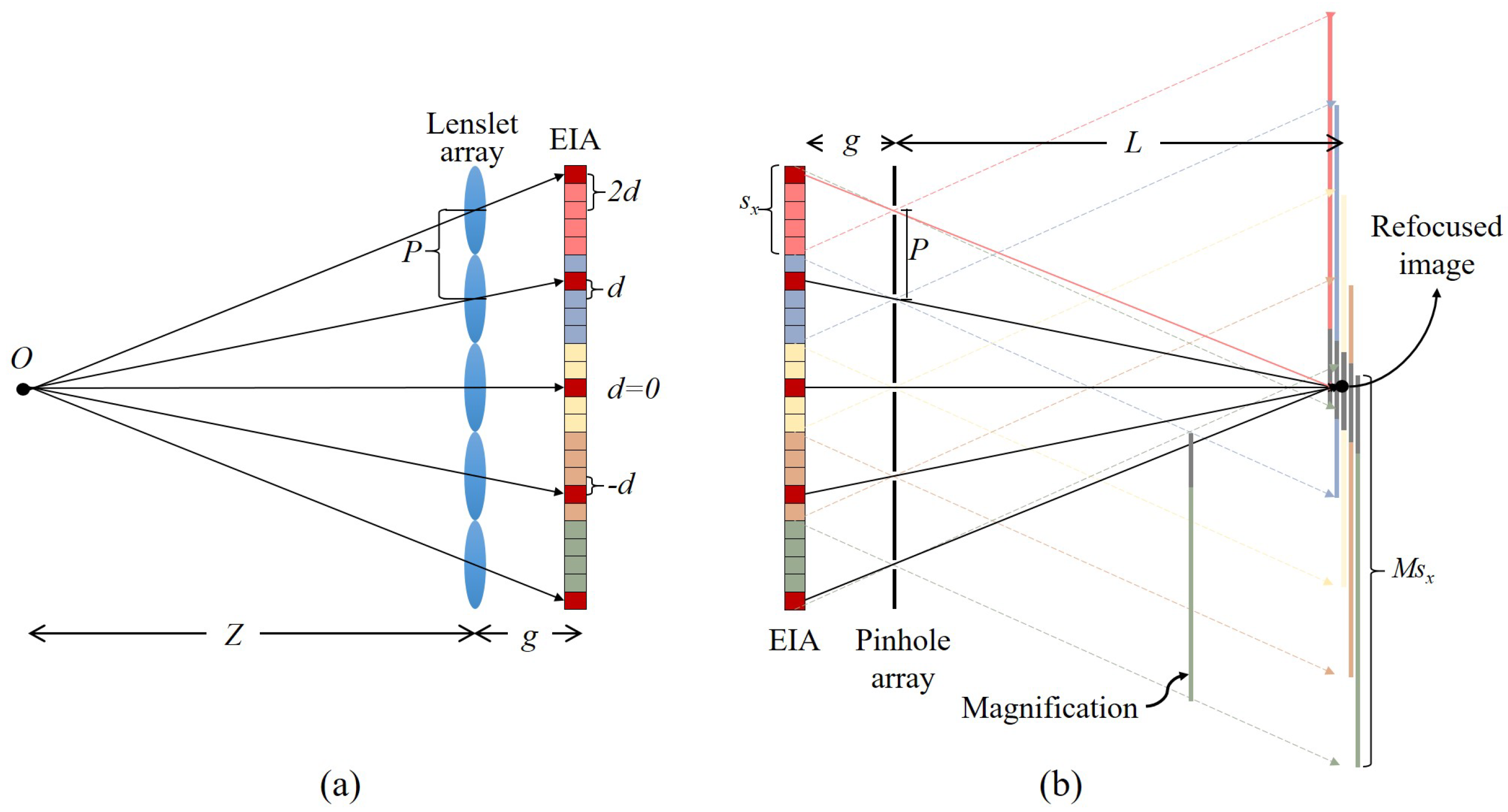
2. Numerical Reconstruction of the Integral Imaging

2.1. Conventional Numerical Reconstruction Method

To understand the conventional numerical reconstruction of II, the conceptual diagram of both procedures is described in Figure 1.

Figure 1a shows the acquisition procedure of EIA to use the single point O. Here, Z is the distance between a single point O and the lenslet array plane. g denotes the distance between the lenslet array and the capturing device. In addition, the parameter P is an interval between neighborhood lenslets. L is the distance between the plane of the virtual pinhole array and the reconstruction plane. ${\mathit{s}}_x$ is the the number of pixels (resolution) of each EI.

In the acquisition procedure, rays emanating from a single point O are passed through each lenslet and recorded on the red-colored pixel. When whole recorded rays through the corresponding lenslet are formed as an individual projection image, this image becomes the EI, and the EIA is formed by the group of EIs. However, each position of the red-colored pixel in each EI is different according to the relative position of the lenslet. This position difference is called the disparity d, which is expressed as d = gP/Z. The feature of this disparity is generally analyzed in the stereo camera-based system [39]. In addition, the EIA capturing procedure based on the lenslet array can be considered as the multiple cameras with P. Therefore, the position difference of the red-colored pixel in arbitrary neighboring EIs constantly remains as d, as shown in Figure 1a.

In the numerical reconstruction procedure of the conventional method, the virtual pinhole array and the acquired EIA are used, as shown in Figure 1b. Here, the acquired EIA is displayed at the EIA plane, and each EI is inversely propagated through the corresponding virtual pinhole along the longitudinal direction. Each inversely propagated EI is magnified according to the magnification factor M, which is expressed as M = L/g [11]. In other words, the number of pixels of the magnified EI becomes M${\mathit{s}}_x$ by the interpolation since the number of pixels of each EI is ${\mathit{s}}_x$. After these magnified EIs are superimposed at the reconstruction plane L together, the single point located at the reconstruction plane is numerically reconstructed.

In the conceptual diagram, the reconstructed single point means that the position difference of each red-colored pixel in every magnified EI becomes 0. In other words, d in two arbitrary adjacent magnified EIs becomes 0. Thus, the condition of d becoming 0 can be treated as the reconstruction condition for the numerical reconstruction in the conventional method. Furthermore, the relation of M = L/g can be derived based on the reconstruction condition.

In the conventional method, the interpolation for the magnification is employed and applied to each EI during the numerical reconstruction. However, the interpolation process for every EI increases the computation time. To overcome this problem, we will explain how to accelerate the computation time of the numerical reconstruction of II under the reconstruction condition in the next section.

2.2. Proposed Numerical Reconstruction

For the acceleration of computation time, the proposed method employs the determined interval mapping in which the interval of each EI is variable depending on the reconstruction plane. Additionally, the proposed method does not require the interpolation process for the magnifying EI during the reconstruction procedure. Since interpolation is not used, the computation time for the numerical reconstruction of II can be reduced. Figure 2 shows the process of the proposed numerical reconstruction.

The EIA from the 3D object is acquired by the acquisition procedure in the same way as the conventional method. The acquired EIA is virtually displayed at the EIA plane, and the virtual pinhole array is located in front of the display EIA. Rays from each displayed EI are passed through the corresponding pinhole, and the flipped EIs are formed. Then, the determined interval $\Delta \tau$ is calculated depending on the reconstruction plane. Each flipped EI is shifted to match $\Delta \tau$ at the reconstruction plane and overlaid with the others to form the superimposed image. However, this superimposed image involves the grid noise caused by the different occurrences of the superposition of each shifted EI. Thus, the superimposed image is divided by the number of occurrences of the superposition to remove the grid noise. Then, the position error between the location of the shifted EI and the pixel position of the reconstruction plane is corrected by inter.polation. Consequently, the refocused image without the grid noise and the position error is numerically reconstructed according to the reconstruction plane.

In the proposed method, the determined interval $\Delta \tau$ is an important factor to reduce the computation time. Thus, the determined interval $\Delta \tau$ can be induced from the image formation model, as shown in Figure 3.

As shown in Figure 3, g is the distance between the displayed EIA plane and the plane of the virtual pinhole array. L is the distance of the reconstruction plane from the virtual pinhole array. The total number of EIs is $\mathit{K}$, and these EIs arranged from (0)^th EI to (K$-1)$^th EI are displayed. In addition, the position difference of the red-colored pixels in adjacent EIs constantly remains as d, as shown in Figure 1.

In the image formation model, each plane of the virtual pinhole array and displayed EIA is located at 0 and −g, respectively. Thus, the position of the red-colored pixel in the displayed (K$-1)$^th and (K$-2)$^th EI is expressed as {−g, (K−1)P+(K−1)d} and {−g, (K−2)P + (K−2)d}, respectively. When rays propagated from each red-colored pixel are inversely mapped at +g, each flipped EI is formed, and its interval remains as P. Hence, the red-colored pixel position of the flipped (K$-1)$^th and (K$-2)$^th EI can be expressed as {g, (K−1)P− (K−1)d} and {g, (K−2)P− (K−2)d}. When each flipped EI is shifted according to $\Delta \tau$ at the reconstruction plane, each red-colored pixel position in the shifted (K$-1)$^th and (K$-2)$^th EI becomes {L, (K−1)$\Delta \tau$− (K−1)d} and {L, (K−2)$\Delta \tau$− (K−2)d}. By the reconstruction condition, the relation of {L, (K−1)$\Delta \tau$− (K−1)d} = {L, (K−2)$\Delta \tau$− (K−2)d} must be satisfied for the numerical reconstruction. Through this relation, the determined interval $\Delta \tau$ depending on the reconstruction plane can be induced in Equation (1).

$$\Delta \tau =\frac{g}{L}P$$

(1)

From Equation (1), we can realize that the determined interval $\Delta \tau$ is determined by the ratio between the g and L. In other words, the $\Delta \tau$ is inversely proportional to the magnification factor M because of the relation of M = L/g. Hence, when the reconstruction plane moves further away from the virtual pinhole array, the calculated value of the interval $\Delta \tau$ becomes smaller.

The number of pixels of the refocused image is different according to the conventional and proposed method. In the conventional method, the resolution ${\mathit{S}}_{\mathit{c}}(\mathit{x},\mathit{y};\mathit{L})$ of the refocused image at the distance $\mathit{L}$ can be expressed as {($K_x+M-1)s_x,(K_y+M-1)s_y$} when $K_x$ and $K_y$ are the total numbers of EIs along $\mathit{x}$- and $\mathit{y}$-direction. If the reconstruction plane L is increased, the resolution of ${\mathit{S}}_{\mathit{c}}(\mathit{x},\mathit{y};\mathit{L})$ will also increase due to the relationship between M and L, where M = L/g. However, since the proposed method does not use interpolation to magnify each EI, the number of pixels of each shifted EI is not changed regardless of the distance $\mathit{L}$. Thus, the number of pixels ${\mathit{S}}_{\mathit{p}}(\mathit{x},\mathit{y};\mathit{L})$ of the superimposed image by the proposed method is expressed as

$${\mathit{S}}_{\mathit{p}}(\mathit{x},\mathit{y};\mathit{L})=\left(\frac{K_x+M-1}{M}\times s_x,\frac{K_y+M-1}{M}\times s_y\right)$$

(2)

In Equation (2), we can realize that ${\mathit{S}}_{\mathit{p}}(\mathit{x},\mathit{y};\mathit{L})$ of the superimposed image is inversely proportional to the value $\mathit{M}$. Thus, ${\mathit{S}}_{\mathit{p}}(\mathit{x},\mathit{y};\mathit{L})$ in the proposed method decreases depending on the increasing reconstruction plane L because of the relation of $\mathit{M}$ = L/g. Additionally, when the reconstruction plane L is moving close to the virtual pinhole array, ${\mathit{S}}_{\mathit{p}}(\mathit{x},\mathit{y};\mathit{L})$ increases. This variation of ${\mathit{S}}_{\mathit{p}}(\mathit{x},\mathit{y};\mathit{L})$ can affect the computation time during the numerical reconstruction of II.

2.3. Position Error Compensation and Adaptive Normalization

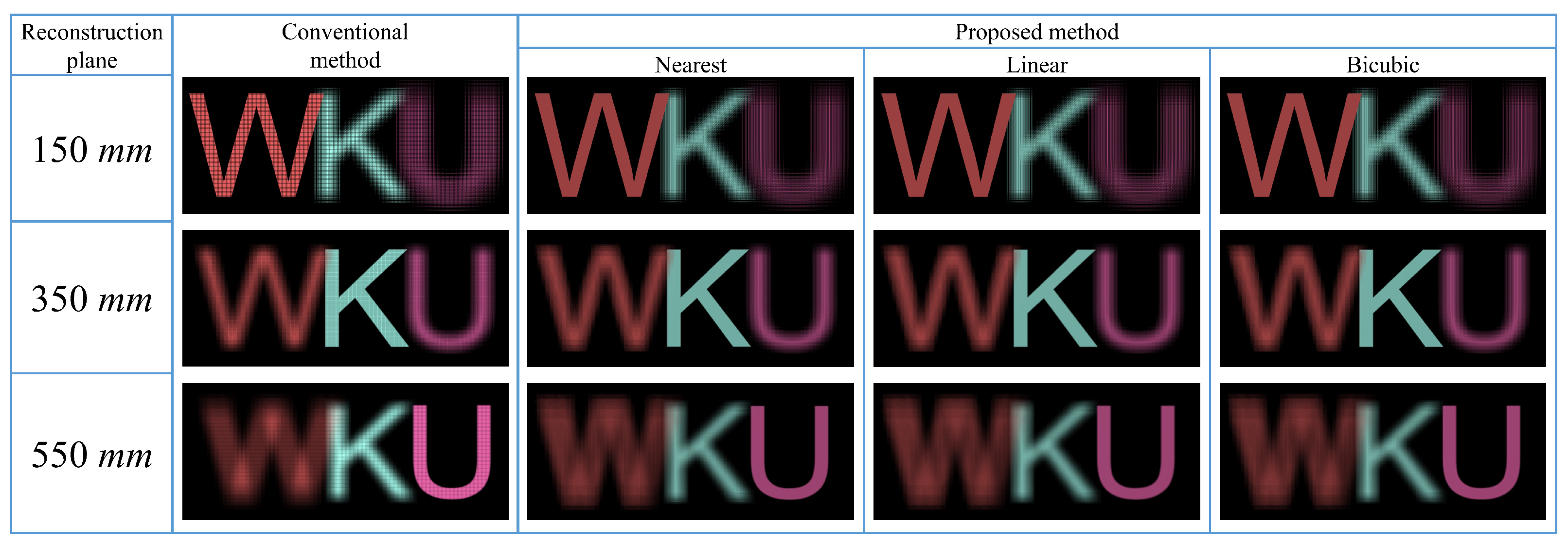
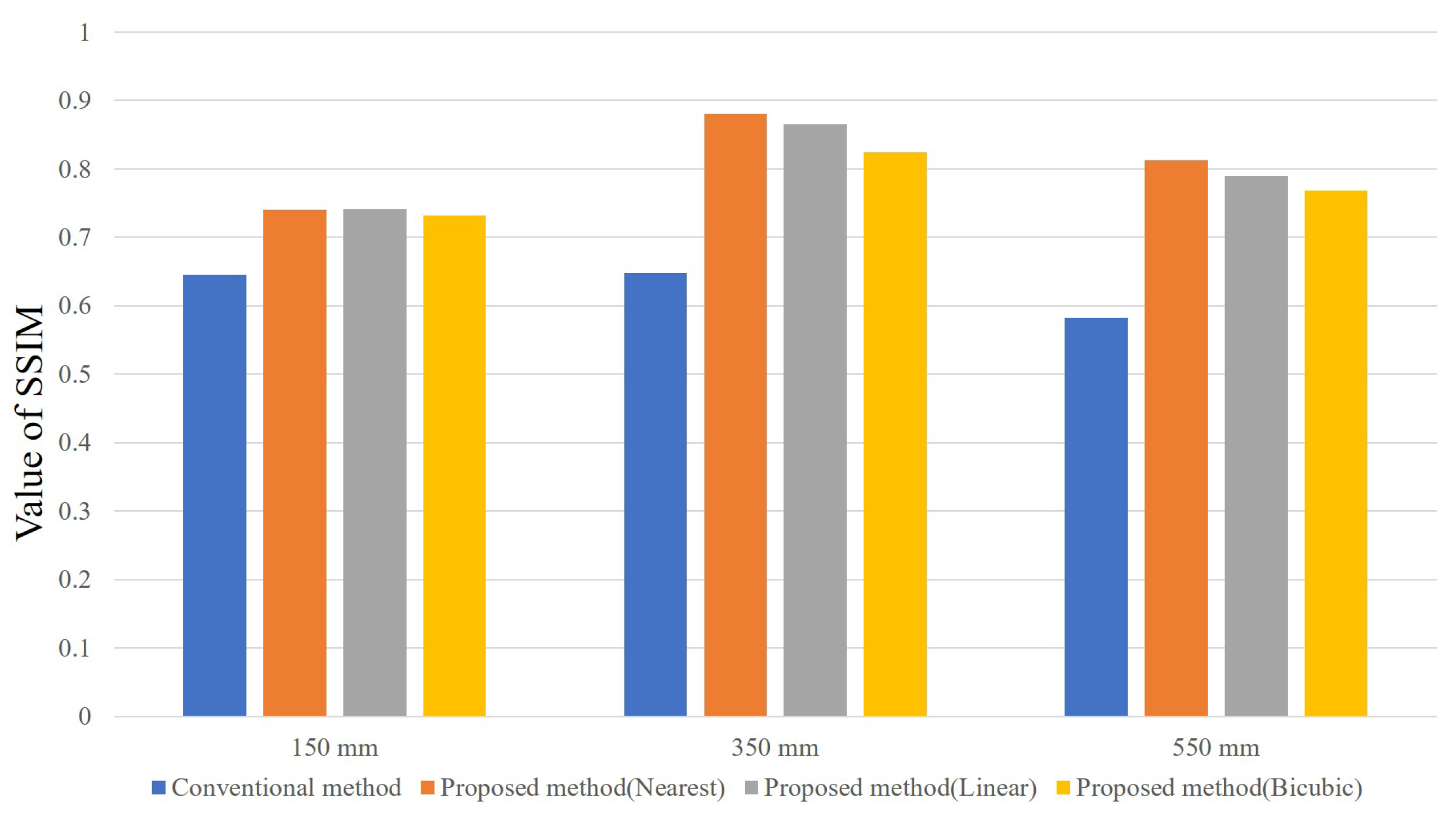
Figure 4 shows a process for the compensation of the position error and the use of adaptive normalization.

When each flipped EI is shifted by the determined interval $\Delta \tau$, the shifted EIs should be mapped in non-integer pixel locations at the reconstruction plane. The position error $\Delta {\mathit{x}}_{\mathit{e}}$ between the non-integer pixel locations of the shifted EI and the integer pixel location of the reconstruction plane appears. Thus, this position error $\Delta {\mathit{x}}_{\mathit{e}}$ has to be corrected. Prior to the compensation of the position error, the pixels of shifted EIs are rounded down to the nearest integer pixel. These EIs are overlaid with the others to form the superimposed image, and then this image is divided by the number of the superposition. This process can be called an adaptive normalization used to remove the grid noise caused by the unequal superposition. After applying adaptive normalization, the position error in the superimposed image is corrected using interpolation because the interpolation method can estimate the value of the non-integer pixel location. As a result, the refocused image with the correction of position error and grid noise is finally reconstructed.

3. Results

3.1. Numerical Experiment

To verify the validity of the proposed method, a numerical experiment was carried out. Figure 5 shows the 3D object used in the numerical experiment and its acquired EIA.

As depicted in Figure 5a, three letters with ‘W’, ‘K’, and ‘U’ utilized by the 3ds Max are used as the virtual 3D object. Each letter is located at a distance of 150 mm, 350 mm, and 550 mm from the virtual lenslet array, respectively; 96 × 54 lenslets are used, and the interval of each elemental lenslet and its FOV is 10 mm and ${10}^{\circ }$. The EIA is acquired by the computational acquisition procedure as shown in Figure 5b. The number of pixels of each EI is 45 × 45. Thus, the number of pixels of the acquired EIA is 4320 × 2430.

For the numerical reconstruction procedure, hardware with an Intel(R) Core(TM) i9-9900KF CPU, 32.0GB ram, and solid-state drive (SSD) is used. Visual studio 2019 and Open CV are used to implement the conventional and proposed method. The number of the virtual pinholes is 96 × 54 to match the number of the virtual lenslets, and the interval of each pinhole is 10 mm, which is the same as the pickup lenslet. The value of g between the virtual pinhole array and the displayed EIA is 57.15 mm.

In the numerical experiment, each reconstruction plane of three letters with ‘W’, ‘K’, and ‘U’ is set up as 150 mm, 350 mm, and 550 mm. In the conventional numerical reconstruction, each value of M related to ‘W’, ‘K’, and ‘U’ is calculated as 2.62, 6.12, and 9.62, respectively. Thus, each EI will be magnified as much as the calculated corresponding value of M. In addition, the number of pixels of each reconstructed image by the conventional method is 4394 × 2504, 4551 × 2661, and 4709 × 2819 in order of the reconstruction plane. In the proposed method, each value of the determined interval $\Delta \tau$ is 3.81 mm, 1.63 mm, and 1.04 mm by Equation (1). Thus, the number of pixels of the numerical reconstruction by the proposed method is 1660 × 946, 710 × 416, and 425 × 257, respectively. Figure 6 shows three kinds of the refocused images reconstructed by the conventional and proposed method to use the nearest, linear, and bicubic interpolation.

When the reconstruction plane is set up as 150 mm, the focused ‘W’ is reconstructed by whole numerical reconstruction methods. In addition, the refocused letters ‘K’ and ‘U’ are visualized when the reconstructed plane is 350 mm and 550 mm, respectively. From these numerical experiments, the proposed method can numerically reconstruct the 3D image depending on the reconstruction plane of the objects ‘W’, ‘K’, and ‘U’. From the experimental result in Figure 6, we can confirm that the proposed method can numerically reconstruct the 3D image similar to the conventional method. Additionally, each reconstructed image has no grid noise in the proposed method because the grid noise is removed by adaptive normalization. To analyze the performance of computation time in whole methods, the comparison of the measured computation time was carried out, as shown in Figure 7.

The x-axis means the value of the reconstruction plane ranging from 100 mm to 700 mm, and the y-axis is the computation time (milliseconds, ms). The blue-colored bar is the computation time by the conventional method, and the orange-, gray-, and yellow-colored bars indicate the individual computation time of the proposed method to employ three different kinds of interpolation methods.

As shown in Figure 7, the computation time represented by the blue-colored bar steadily increases in compliance with the increasing reconstruction plane because each EI is magnified as much as M times. Moreover, the increasing reconstruction plane causes a huge memory requirement related to the resolution of the refocused image. Thus, the computation time of the conventional method increases depending on the interpolation for the magnification and the high memory size.

However, each computation time described by the orange-, gray-, and yellow-colored bars is steadily reduced when the reconstruction plane moves far from the virtual pinhole array. This means that the interpolation time for each EI is not added to the computation time while the refocused image is numerically reconstructed. In addition, the memory size related to the resolution of the refocused image is smaller than the conventional method. Therefore, the total computation time in the proposed method can be relatively faster than the conventional method.

3.2. Quality Comparison of the Reconstructed Image

The structural similarity index measure (SSIM) is a useful method to predict image quality based on features of the human visual system [40,41,42]. Therefore, the SSIM was employed to quantitatively evaluate the quality of each refocused image by the conventional method and the proposed methods.

To calculate the SSIM value, three kinds of single letters of “W”, “K”, and “U” located at 150 mm, 350 mm, and 550 mm are modeled by the 3ds max software. Then, each EIA from each letter is acquired by the computational capturing method. Figure 8 shows the individual EIA acquired from a single letter of “W”, “K”, and “U” and the corresponding EIAs.

All specifications relating to the acquired EIAs are the same as the previous experiment.

Figure 9 shows each refocused image by the conventional and proposed methods for the calculation of the SSIM value.

Three reference images are on the left of Figure 9. Three reconstructed letters ‘W’, ‘K’, and ‘U’ by the conventional method at the corresponding reconstruction plane are positioned in the two columns of Figure 9. In 3∼5 columns and 1 to 3 rows, each reconstructed letter ‘W’, ‘K’, and ‘U’ by the use of the three different interpolation methods in the proposed method is visualized, depending on the corresponding reconstruction plane. To ensure consistency in the calculation of the SSIM, the resolution of each refocused image has been set to 3840 × 2160 pixels because the number of pixels of each refocused image is different. Each SSIM value between each reference image and its corresponding refocused image is measured, and the calculated SSIM value is shown in Figure 10.

In Figure 10, the x-axis is three reconstruction planes with 150 mm, 350 mm, and 550 mm, and the y-axis corresponds to the SSIM value. The blue-colored bar indicates the SSIM value of each refocused image by the conventional method, and the orange-, gray-, and yellow-colored bars indicate the individual value of the SSIM between each reference image and refocused image by the proposed method with the nearest, linear, and bicubic interpolation. As shown in Figure 10, the SSIM values of refocused images by the conventional method are 0.646, 0.648, and 0.582 at 150 mm, 350 mm, and 550 mm. However, the individual SSIM value of the refocused letters ‘W’, ‘K’, and ‘U’ in the proposed method with the use of the nearest interpolation represents 0.740, 0.881, and 0.813 at 150 mm, 350 mm, and 550 mm, respectively. When linear interpolation is used in the proposed method, the SSIM values between the reference and refocused images are 0.741, 0.865, and 0.789 at the same distances. Similarly, the proposed method using bicubic interpolation yields SSIM values of 0.733, 0.825, and 0.769 at distances of 150 mm, 350 mm, and 550 mm, respectively.

In order to compare the qualitative quality of the refocused image, the numerical experiment was performed employing a 3D model of a dragon with continuous depth and fine texture, as shown in Figure 11.

Figure 11a illustrates the rendered dragon featuring a rich texture on its surface. Additionally, the range of this 3D modeling spans from 120 mm to 550 mm in the $\mathit{z}$-direction. After the EIA was acquired from this rendered dragon, each refocused image reconstructed by the conventional and proposed method is shown in Figure 11b, and the four different reconstruction planes are 170 mm, 240 mm, 310 mm, and 380 mm, respectively. When the conventional method is utilized, the refocused image contains grid noise resulting in reduced visibility of the texture of the 3D model, as depicted at the top of Figure 11b. Thus, the qualitative quality of the refocused image is noticeably low. However, the refocused images reconstructed by the proposed method involve the enhanced visibility of the texture compared to the conventional method because the grid noise is effectively eliminated. In addition, the kinds of interpolation employed in the proposed method do not result in any noticeable difference in the qualitative quality of each refocused image at the same reconstruction plane. From these experimental results, we can conclude that the proposed method reconstructs refocused images with better visual quality than the conventional method.

4. Conclusions

In this paper, a fast numerical reconstruction of II based on a determined interval mapping is proposed for reducing computation time. The proposed method does not require the magnification process by interpolation and large memory size during the numerical reconstruction of II. Accordingly, the computation time can be reduced significantly. To achieve the proposed method, the displayed EIs through the corresponding virtual pinhole are first transformed into flipped EIs. These flipped EIs are shifted to match the determined interval calculated depending on the reconstruction plane and superimposed together. After this superimposed image is divided by the number of the superposition, the position error between the location of the shifted EI and the pixel position of the reconstruction plane is corrected by interpolation. Finally, the refocused image is reconstructed based on the relatively short computation time. To validate the feasibility of the proposed method, two numerical experiments related to the computation time and the quality comparison of each refocused image were carried out. By conducting an experiment to measure computation time, the proposed method can yield a refocused image faster than the conventional method. Furthermore, the computational time of the proposed method varies slightly depending on the type of interpolation, such as the nearest, linear, and bicubic methods. To accurately measure the reconstruction quality, the SSIM was used to compare the quantitative quality measurement between the reference image and each reconstructed image. Through the experimental result, we confirmed that the proposed method outperforms the conventional method in terms of reconstruction quality, regardless of the type of interpolation used. From both numerical experiments, we confirmed that the proposed method can improve the computation time and the numerical reconstruction quality.

References

1. Okano, F.; Hoshino, H.; Arai, J.; Yuyama, I. Real-time pickup method for a three-dimensional image based on integral photography. Appl. Opt. 1997, 36, 1598–1603. [Google Scholar] [CrossRef] [PubMed]
2. Lee, B.; Jung, S.; Park, J.H. Viewing-angle-enhanced integral imaging by lens switching. Opt. Lett. 2002, 27, 818–820. [Google Scholar] [CrossRef]
3. Stern, A.; Javidi, B. Three-dimensional image sensing and reconstruction with time-division multiplexed computational integral imaging. Appl. Opt. 2003, 42, 7036–7042. [Google Scholar] [CrossRef] [PubMed] [Green Version]
4. Piao, Y.; Xing, L.; Zhang, M.; Lee, M.C. Resolution enhanced computational integral imaging reconstruction by using boundary folding mirrors. J. Opt. Soc. Korea 2016, 20, 363–367. [Google Scholar] [CrossRef] [Green Version]
5. Choi, H.M.; Choi, J.G.; Kim, E.S. Off-axis multi-projection integral imaging with calibrated elemental image arrays based on pixel-position mapping. Ict Express 2018, 4, 112–117. [Google Scholar] [CrossRef]
6. Yan, Z.; Yan, X.; Huang, Y.; Jiang, X.; Yan, Z.; Liu, Y.; Mao, Y.; Qu, Q.; Li, P. Characteristics of the holographic diffuser in integral imaging display systems: A quantitative beam analysis approach. Opt. Lasers Eng. 2021, 139, 106484. [Google Scholar] [CrossRef]
7. Qin, Z.; Zhang, Y.; Yang, B.R. Interaction between sampled rays’ defocusing and number on accommodative response in integral imaging near-eye light field displays. Opt. Express 2021, 29, 7342–7360. [Google Scholar] [CrossRef]
8. Wang, W.; Chen, G.; Weng, Y.; Weng, X.; Zhou, X.; Wu, C.; Guo, T.; Yan, Q.; Lin, Z.; Zhang, Y. Large-scale microlens arrays on flexible substrate with improved numerical aperture for curved integral imaging 3D display. Sci. Rep. 2020, 10, 1–9. [Google Scholar] [CrossRef]
9. Choi, J.G.; Choi, H.M.; Hwang, Y.S.; Kim, E.S. Real-time sensing and three-dimensional display of far outdoor scenes based on asymmetric integral imaging. Opt. Lasers Eng. 2017, 94, 44–57. [Google Scholar] [CrossRef]
10. Takaki, Y.; Yamaguchi, Y. Flat-panel see-through three-dimensional display based on integral imaging. Opt. Lett. 2015, 40, 1873–1876. [Google Scholar] [CrossRef]
11. Hong, S.H.; Jang, J.S.; Javidi, B. Three-dimensional volumetric object reconstruction using computational integral imaging. Opt. Express 2004, 12, 483–491. [Google Scholar] [CrossRef] [PubMed]
12. Shin, D.H.; Kim, E.S.; Lee, B. Computational reconstruction of three-dimensional objects in integral imaging using lenslet array. Jpn. J. Appl. Phys. 2005, 44, 8016. [Google Scholar] [CrossRef]
13. Arimoto, H.; Javidi, B. Integral three-dimensional imaging with digital reconstruction. Opt. Lett. 2001, 26, 157–159. [Google Scholar] [CrossRef]
14. Frauel, Y.; Javidi, B. Digital three-dimensional image correlation by use of computer-reconstructed integral imaging. Appl. Opt. 2002, 41, 5488–5496. [Google Scholar] [CrossRef] [PubMed]
15. Hong, S.H.; Javidi, B. Improved resolution 3D object reconstruction using computational integral imaging with time multiplexing. Opt. Express 2004, 12, 4579–4588. [Google Scholar] [CrossRef]
16. Li, H.; Wang, S.; Zhao, Y.; Wei, J.; Piao, M. 3D view image reconstruction in computational integral imaging using scale invariant feature transform and patch matching. Opt. Express 2019, 27, 24207–24222. [Google Scholar] [CrossRef]
17. Bae, J.; Yoo, H. Review and Comparison of Computational Integral Imaging Reconstruction. Int. J. Appl. Eng. Res. 2019, 14, 250–253. [Google Scholar]
18. Cho, M.; Javidi, B. Computational reconstruction of three-dimensional integral imaging by rearrangement of elemental image pixels. J. Disp. Technol. 2009, 5, 61–65. [Google Scholar] [CrossRef]
19. Shin, D.H.; Lee, B.; Kim, E.S. Improved Viewing Quality of 3-D Images in Computational Integral Imaging Reconstruction Based on Lenslet Array Model. ETRI J. 2006, 28, 521–524. [Google Scholar] [CrossRef]
20. Shin, D.H.; Yoo, H. Image quality enhancement in 3D computational integral imaging by use of interpolation methods. Opt. Express 2007, 15, 12039–12049. [Google Scholar] [CrossRef]
21. Inoue, K.; Lee, M.C.; Javidi, B.; Cho, M. Improved 3D integral imaging reconstruction with elemental image pixel rearrangement. J. Opt. 2018, 20, 025703. [Google Scholar] [CrossRef]
22. Inoue, K.; Cho, M. Visual quality enhancement of integral imaging by using pixel rearrangement technique with convolution operator (CPERTS). Opt. Lasers Eng. 2018, 111, 206–210. [Google Scholar] [CrossRef]
23. Kim, H.; Lee, S.; Ryu, T.; Yoon, J. Superresolution of 3-D computational integral imaging based on moving least square method. Opt. Express 2014, 22, 28606–28622. [Google Scholar] [CrossRef] [PubMed]
24. Yoo, H.; Jang, J.Y. Intermediate elemental image reconstruction for refocused three-dimensional images in integral imaging by convolution with δ-function sequences. Opt. Lasers Eng. 2017, 97, 93–99. [Google Scholar] [CrossRef]
25. Bae, K.H.; Kim, E.S. New disparity estimation scheme based on adaptive matching windows for intermediate view reconstruction. Opt. Eng. 2003, 42, 1778–1786. [Google Scholar] [CrossRef]
26. Shin, D.H.; Yoo, H. Scale-variant magnification for computational integral imaging and its application to 3D object correlator. Opt. Express 2008, 16, 8855–8867. [Google Scholar] [CrossRef]
27. Hwang, D.C.; Shin, D.H.; Kim, S.C.; Kim, E.S. Depth extraction of three-dimensional objects in space by the computational integral imaging reconstruction technique. Appl. Opt. 2008, 47, D128–D135. [Google Scholar] [CrossRef]
28. Llavador, A.; Sánchez-Ortiga, E.; Saavedra, G.; Javidi, B.; Martínez-Corral, M. Free-depths reconstruction with synthetic impulse response in integral imaging. Opt. Express 2015, 23, 30127–30135. [Google Scholar] [CrossRef] [Green Version]
29. Jang, J.Y.; Ser, J.I.; Cha, S.; Shin, S.H. Depth extraction by using the correlation of the periodic function with an elemental image in integral imaging. Appl. Opt. 2012, 51, 3279–3286. [Google Scholar] [CrossRef]
30. Wu, C.; McCormick, M.; Aggoun, A.; Kung, S.Y. Depth mapping of integral images through viewpoint image extraction with a hybrid disparity analysis algorithm. J. Disp. Technol. 2008, 4, 101–108. [Google Scholar]
31. Xiao, X.; Daneshpanah, M.; Javidi, B. Occlusion removal using depth mapping in three-dimensional integral imaging. J. Disp. Technol. 2012, 8, 483–490. [Google Scholar] [CrossRef]
32. Shen, X.; Markman, A.; Javidi, B. Three-dimensional profilometric reconstruction using flexible sensing integral imaging and occlusion removal. Appl. Opt. 2017, 56, D151–D157. [Google Scholar] [CrossRef] [PubMed]
33. Ryu, T.; Lee, B.; Lee, S. Mutual constraint using partial occlusion artifact removal for computational integral imaging reconstruction. Appl. Opt. 2015, 54, 4147–4153. [Google Scholar] [CrossRef]
34. Yoo, H. Depth extraction for 3D objects via windowing technique in computational integral imaging with a lenslet array. Opt. Lasers Eng. 2013, 51, 912–915. [Google Scholar] [CrossRef]
35. Zhang, M.; Piao, Y.; Wei, C.; Si, Z. Occlusion removal based on epipolar plane images in integral imaging system. Opt. Laser Technol. 2019, 120, 105680. [Google Scholar] [CrossRef]
36. Yoo, H.; Shin, D.; Cho, M. Improved depth extraction method of 3D objects using computational integral imaging reconstruction based on multiple windowing techniques. Opt. Lasers Eng. 2015, 66, 105–111. [Google Scholar] [CrossRef]
37. Yi, F.; Moon, I.; Lee, J.A.; Javidi, B. Fast 3D computational integral imaging using graphics processing unit. J. Disp. Technol. 2012, 8, 714–722. [Google Scholar] [CrossRef]
38. Hong, S.; Incardona, N.; Inoue, K.; Cho, M.; Saavedra, G.; Martinez-Corral, M. GPU-accelerated integral imaging and full-parallax 3D display using stereo–plenoptic camera system. Opt. Lasers Eng. 2019, 115, 172–178. [Google Scholar] [CrossRef]
39. Park, J.H.; Kim, Y.; Kim, J.; Min, S.W.; Lee, B. Three-dimensional display scheme based on integral imaging with three-dimensional information processing. Opt. Express 2004, 12, 6020–6032. [Google Scholar] [CrossRef]
40. Wang, Z.; Bovik, A.C.; Sheikh, H.R.; Simoncelli, E.P. Image quality assessment: From error visibility to structural similarity. IEEE Trans. Image Process. 2004, 13, 600–612. [Google Scholar] [CrossRef] [Green Version]
41. Alam, M.; Kwon, K.C.; Erdenebat, M.U.; Abbass, M.Y.; Kim, N. Super-resolution enhancement method based on generative adversarial network for integral imaging microscopy. Sensors 2021, 21, 2164. [Google Scholar] [CrossRef] [PubMed]
42. Huo, W.; Sang, X.; Xing, S.; Guan, Y.; Li, Y. Backward ray tracing based rectification for real-time integral imaging display system. Opt. Commun. 2020, 458, 124752. [Google Scholar] [CrossRef]
Figure 1. The conceptual diagram of both procedures in the conventional numerical reconstruction method based on the single point O. (a) Acquisition procedure; (b) numerical reconstruction procedure.
Applsci 13 06942 g001
Figure 2. Conceptual configuration of the proposed method.
Applsci 13 06942 g002
Figure 3. Image formation model for the proposed numerical reconstruction.
Applsci 13 06942 g003
Figure 4. Process for the compensation of the position error and the use of adaptive normalization.
Applsci 13 06942 g004
Figure 5. (a) Computational II pickup for three letters of ‘W’, ‘K’, and ‘U’; (b) acquired EIA.
Applsci 13 06942 g005
Figure 6. Refocused image by the conventional method and the proposed method with the use of the three interpolation methods at 150 mm, 350 mm, and 550 mm.
Applsci 13 06942 g006
Figure 7. Comparison of the total computation time of the conventional and proposed method.
Applsci 13 06942 g007
Figure 8. Three kinds of letters of ‘W’, ‘K’, and ‘U’ and their EIAs located at (a) 150 mm, (b) 350 mm, and (c) 550 mm.
Applsci 13 06942 g008
Figure 9. Reference and each refocused image by the conventional and proposed methods by use of the different interpolations.
Applsci 13 06942 g009
Figure 10. Measured SSIM values of each reconstructed image.
Applsci 13 06942 g010
Figure 11. Comparison of the qualitative quality of the refocused image: (a) front and top views of the rendered 3D model with the continuous depth range; (b) refocused images reconstructed by the conventional and proposed methods employing nearest, linear, and bicubic interpolation at each reconstruction plane of 170 mm, 240 mm, 310 mm, and 380 mm.
Applsci 13 06942 g011
Disclaimer/Publisher’s Note: The statements, opinions and data contained in all publications are solely those of the individual author(s) and contributor(s) and not of MDPI and/or the editor(s). MDPI and/or the editor(s) disclaim responsibility for any injury to people or property resulting from any ideas, methods, instructions or products referred to in the content.