Design of an Intelligent Vehicle Behavior Decision Algorithm Based on DGAIL

Abstract

With the development of AI, the intelligence level of vehicles is increasing. Structured roads, as common and important traffic scenes, are the most typical application scenarios for realizing autonomous driving. The driving behavior decision-making of intelligent vehicles has always been a controversial and difficult research topic. Currently, the mainstream decision-making methods, which are mainly based on rules, lack adaptability and generalization to the environment. Aimed at the particularity of intelligent vehicle behavior decisions and the complexity of the environment, this thesis proposes an intelligent vehicle driving behavior decision method based on DQN generative adversarial imitation learning (DGAIL) in the structured road traffic environment, in which the DQN algorithm is utilized as a GAIL generator. The results show that the DGAIL method can preserve the design of the reward value function, ensure the effectiveness of training, and achieve safe and efficient driving on structured roads. The experimental results show that, compared with A3C, DQN and GAIL, the model based on DGAIL spends less average training time to achieve a 95% success rate in the straight road scene and merging road scene, respectively. Apparently, this algorithm can effectively accelerate the selection of actions, reduce the randomness of actions during the exploration, and improve the effect of the decision-making model.

1. Introduction

Smart cars are listed as one of the key development objects in the Made in China 2025 Plan and are defined as a new generation of vehicles with Internet of Vehicles communication and intelligent driving ability. The main task is to improve the safety, comfort, energy savings, and efficiency of driving and to promote the development of comprehensive transportation [1]. An intelligent driving system is generally composed of an environment perception layer, decision planning layer, and action control layer [2]. As shown in Figure 1, the environment perception layer is the “eye” of the intelligent vehicle; the decision-making and planning layer is the “brain” of the intelligent vehicle. After receiving the data from the environment perception layer, the independent data information in time and space is converted to the behavior decision and planning path of the vehicle. The action control layer is the “hand and foot” of the intelligent vehicle. The decision-making and planning layer is the core of the smart car. In an automatic driving system with high requirements in terms of safety, real-time, rapidity, and predictability, the rationality of behavioral decision-making will directly affect the safety and comfort of the vehicle and its economy. The driving decision-making algorithm directly reflects the technical level of the decision-making and planning layer. Therefore, the development of autonomous driving technology is important for investigating the driving behavior decision-making algorithm of intelligent vehicles and for improving the intelligence level of vehicles.

Presently, there are three main decision-making methods for intelligent vehicles, namely, rule-based decision-making methods, “end-to-end” decision-making methods, and decision-making methods based on deep reinforcement learning. Deep reinforcement learning is similar to the process of humans learning new knowledge. In continuous interaction with the environment, the agent uses the rewards or punishments that are obtained to continuously optimize the strategy until it learns the optimal strategy. In 2017, Hyunmin Chae proposed a vehicle braking system based on the DQN algorithm and applied the algorithm to the control of the vehicle braking system [3]. In 2018, Maximilian proposed an intelligent vehicle decision-making system based on the A3C algorithm. The input layer is the image information obtained by a convolutional neural network (CNN). The A3C algorithm is used to train the vehicle in the simulation environment, and good results have been achieved [4]. In 2018, Alex Kendall of Wayve, a self-driving car company, proposed a DDPG-based lane-keeping method. The image information obtained by the monocular camera is input into the CNN, and the DDPG algorithm is used to output the vehicle’s decision-making actions and carry them out; this method has been verified by real vehicles and achieved a better lane tracking effect [5]. In 2018, Fang Chuan proposed the DDPG algorithm, which added a teaching data part to the loss function of DDPG and achieved better results than the DDPG algorithm in the lane-keeping test in the CARLA environment [6]. In 2018, Hoel proposed a self-vehicle overtaking control method based on deep reinforcement learning in dynamic uncertain environments, which can realize lane keeping and autonomous overtaking behaviors in high-speed dynamic scenarios [7]. In 2020, Luo proposed a DQN-based decision-making method in high-speed scenarios, combining the DQN algorithm with expert knowledge, which greatly shortened the training time [8]. Although deep reinforcement learning has performed well in some application scenarios, it still faces the problem of low learning efficiency, and it is difficult to achieve the efficiency shown by humans when solving problems. Imitation learning can learn existing expert knowledge, convert the expert knowledge into learning samples, and use the expert knowledge to guide the training of the agent, which reduces the number of ineffective exploration problems encountered by the agent in the training process and reduces the training time cost and computing cost, effectively improving the learning performance of deep reinforcement learning [9]. There are three commonly used imitation learning methods, namely, behavior cloning, inverse reinforcement learning, and generative adversarial imitation learning. Generative adversarial imitation learning (GAIL) is an imitation learning framework based on a generative adversarial network (GAN), which consists of a generator and a discriminator. The discriminator provides a reward value to the generator by identifying the difference between the expert strategy and the learned strategy. Similarly to the generator training method in the GAN, after obtaining the reward value given by the discriminator, GAIL uses the TRPO and PPO algorithms to carry out strategy training. Generative adversarial imitation learning learns policies from a small number of expert trajectories and uses the discriminator to generate a reward value function, which reduces the demand for training samples and the computational complexity. In 2016, Jonathan Ho [10] proposed generative adversarial imitation learning (GAIL) based on a GAN network. In 2017, Hausman K [11] proposed a multimodal biomimetic learning framework, using a GAN network to establish a multimodal biomimetic learning framework from unstructured and unlabeled teaching samples. In 2017, Merel J [12] proposed a hierarchical strategy framework based on reinforcement learning, using generative adversarial imitation learning to train low-level controllers in the acquired action dataset and reinforcement learning to train high-level controllers. In 2017, Yun Zhu Li [13] proposed infogenerative adversarial imitation learning (Info-Gail), which combined the Info-Gan network with the Gail algorithm so that the agent can better understand the meaning of expert data. In 2018, Jiaming Song [14] proposed multigenerative adversarial imitation learning (Multi-Gail), which combined a multiagent system and the Gail algorithm to extend the Gail algorithm to the multiagent field.

In summary, the depth of the reinforcement learning for the intelligent vehicle behavior decision model has good adaptability and generalization. This paper is based on related research projects. An intelligent vehicle is the research object, and the depth is proposed based on the reinforcement learning method to design an intelligent vehicle frame of decision-making behavior. To conduct thorough research on the decision-making algorithm, the proposed DGAIL was used to study the intelligent decision-making system. The DQN algorithm is proposed to serve as the generation network of GAIL to realize the transformation of the original GAIL algorithm and to make it more suitable for an intelligent vehicle decision-making system.

The research in this paper combines theoretical analysis and simulation experiments. The test platform was built based on the Pygame module. Considering the function of the decision-making system, the scenarios of straight road and merging road in the structured road were selected as the simulation scenarios. By setting road and vehicle parameters, lane keeping, lane changing, on-ramp incorporation, entry and exit roundabouts, and other functions were verified. The behavior decision model based on the DGAIL algorithm was designed to realize autonomous decision-making by intelligent vehicles on structured roads, and the effectiveness and stability of the algorithm in straight and merge scenarios were verified in the simulation environment.

2. Methods

Previous studies have shown that the intelligent vehicle behavior decision algorithm based on DQN can satisfy the requirements of safety, efficiency, and stability of the decision-making system. However, the design of the reward value function is still too cumbersome: a poor reward value function will reduce the success rate and convergence of training, and it is difficult to obtain satisfactory results. This paper proposes a DQN-based generative adversarial imitation learning (DGAIL) method. Using the design structure of GAIL, through the learning of expert data, the design problem of the reward value function of the agent in deep reinforcement learning was solved. The DQN was used to replace the TRPO method to accelerate the training of the model, and the behavior decision model could be quickly constructed to perform intelligent vehicle decision-making training tasks in the simulation environment. The vehicle driving behavior decision-making algorithm designed in this paper is mainly aimed at structured roads and does not involve traffic signals, traffic signs, and pedestrians.

2.1. Improvement of the DGAIL Algorithm

The improvement of the DGAIL algorithm included two aspects. The first aspect was to replace the TRPO method with DQN based on a deterministic strategy to improve the efficiency of sample utilization. The second aspect was to use the the Leaky-ReLU function in the discriminator D to replace the ReLU function and improve the stability of the algorithm.

2.1.1. Generator G Is DQN

The original GAIL method was designed for a continuous state space and continuous action space, and the generator G adopted TRPO [15] or PPO [16] methods based on stochastic policies. For the method based on a random strategy, the action strategy taken by the agent when the state is s obeys a normal distribution, whose mean is ξ and whose variance is σ. The action strategy function can be expressed as:

$${\mathsf{\pi }}_{\mathsf{\theta }}(\mathrm{a},\mathrm{s})=\frac{1}{\sqrt{2\mathsf{\pi }}\mathsf{\delta }}\mathrm{e}\mathrm{x}\mathrm{p}(-\frac{{(\mathrm{a}-\mathsf{\xi })}^2}{2{\mathsf{\delta }}^2})$$

(1)

where s is the state space of the agent, a is the action space of the agent, ${\mathsf{\pi }}_{\mathsf{\theta }}(\mathrm{a},\mathrm{s})$ is the probability density of the action policy function when the agent adopts the action, and the parameters of normal distribution are ξ (mean value) and σ (variance).

For the method based on the random action policy, the gradient can be expressed as:

$${\nabla }_{\mathsf{\theta }}\mathrm{J}({\mathsf{\pi }}_{\mathsf{\theta }})={\mathrm{E}}_{(\mathrm{s},\mathrm{a})~{\mathsf{\pi }}_{\mathsf{\theta }}}\left[{\nabla }_{\mathsf{\theta }}\mathrm{l}\mathrm{o}\mathrm{g}{\mathsf{\pi }}_{\mathsf{\theta }}\left(\mathrm{a}\right|\mathrm{s}\left){\mathrm{Q}}^{{\mathsf{\pi }}_{\mathsf{\theta }}}\right(\mathrm{s},\mathrm{a})\right]$$

(2)

where s is the state space of the agent, a is the action space of the agent, ${\mathsf{\pi }}_{\mathsf{\theta }}(\mathrm{a},\mathrm{s})$ is the probability density of the action policy function when the agent adopts the action, and in the states, ${\mathrm{Q}}^{{\mathsf{\pi }}_{\mathsf{\theta }}}(\mathrm{s},\mathrm{a})$ refers to the expected reward value when the action policy function is ${\mathsf{\pi }}_{\mathsf{\theta }}(\mathrm{a},\mathrm{s})$.

Equations (1) and (2) show that when the agent faces the same state s, the output of the action policy function obeys a normal distribution, and the output value a is different each time. When updating the gradient, the random action strategy fully samples the environment and then calculates the real expected value according to the state distribution and action distribution, which increases the time cost of sampling and reduces the utilization of samples.

If the action space of the agent is discrete, TRPO needs to discretize the output action policy function and then use the softmax function to select the maximum Q value, while the DQN method is based on the deterministic policy acting in the same states. The choice of a is deterministic, and the maximum Q value can be directly and accurately output, which saves the invalid exploration time in the training process. Therefore, in the discrete space scenario set in this paper, the DQN algorithm samples less of the environment during the training process, and the utilization rate of the samples is high, especially for complex discrete systems such as the intelligent vehicle decision model. The DQN algorithm has a low sampling rate. The learning efficiency will be greatly improved.

2.1.2. Activation Function of the Discriminator D

Commonly used activation functions include sigmoid, tanh, ReLU, and leaky-ReLU. The sigmoid function and tanh function are more traditional activation functions, but they may encounter the problem of regional saturation when transmitting information in the neural network, resulting in the phenomenon of gradient disappearance. The ReLU function solves the problem of vanishing gradients, but there is a “dead zone” when the input is negative. The leaky-ReLU function optimizes this zone by assigning a nonzero slope to all negative values of the input, solving the “dead zone” problem of the ReLU function. The ReLU activation function used by the discriminator D in the original GAIL method reduces the influence of the “dead zone” on the training results, as shown in Figure 2. This paper selects leaky ReLU as the activation function between the input layer and the hidden layer.

2.2. GAN Network

In 2014, Goodfellow proposed a generative adversarial network (GAN) [17]. The GAN network consists of generator G and discriminator D. Generator G is used to generate fake samples, its input is noise data Z, and the output is fake sample data. The discriminant Model D is a binary classifier; its input is the expert sample and fake sample, and the output is the true and false probability of the sample data, which is used to distinguish the fake sample data from the expert sample data. The objective function of the generator G is:

$$G={\nabla }_{{\theta }_g}\frac{1}{n}{\displaystyle \sum _{i=1}^n\log (1-D(G(z^i})))$$

(3)

where Z = {z¹, z²..., z^m} is the noise data that generates false samples, and n is the number of samples. Discriminator D guides the training of generator G by identifying the difference between the fake samples and the expert samples of generator G. The objective function of discriminator V(G, D) is:

$$V={\nabla }_{{\theta }_d}\frac{1}{n}{\displaystyle \sum _{i=1}^n[\log D(x^i)+\log (1-D(G(z^i})))]$$

(4)

where n is the number of sample data and X = {x¹, x²..., xⁿ} is the sample data. In the process of model training, the training of generator G and discriminator D is alternately carried out, and the two update their own training parameters through the gradient descent method to reduce the value of the loss function. In continuous training, generator G and discriminator D through the dynamic game form a Nash equilibrium.

2.3. DGAIL Algorithm

The structural model of generative adversarial imitation learning (GAIL) is similar to the GAN. Deep reinforcement learning is utilized as generator G to create fake samples, and a generative adversarial network is employed as discriminator D to identify expert samples and fake samples. In the constant game between generator G and discriminator D, the two reach Nash equilibrium so that generator G obtains the optimal strategy of the model and completes the optimization of the learning model.

This chapter combines the GAIL method and DQN method to propose a DQN-based generative adversarial imitation learning (DGAIL) method. The structural model of DGAIL, which consists of generator G and discriminator D, is shown in Figure 3. The DQN algorithm is used by generator G, and the two-class neural network is used by discriminator D. In the training process of the smart car decision model, generator G uses the DQN algorithm to generate fake samples, and discriminator D judges the authenticity of the expert samples and fake samples and outputs the judgment result as the reward value function of generator G. Through continuous training, generator G and discriminator D play against each other in the training process until the Nash equilibrium state is reached and generator G can generate fake samples.

$$\underset{\psi }{\min }\underset{\theta }{\max }V(\theta ,\varphi )=E_{(s,a)\in {\chi }_E}\left[\log D_{\psi }(s,a)\right]+E_{(s,a)\in {\chi }_{\theta }}\left[\log (1-D_{\psi }(s,a))\right]$$

(5)

$${\chi }_{\theta }=\{(s_1,a_1),(s_2,a_2),\dots ,(s_T,a_T)\}$$

(6)

where s_i represents the state at time i, a_i represents the action at time i, χ_θ represents the “realistic sample” generated by generator G, χ_E represents the expert sample data, and D_ψ represents the discriminator. The structure is shown in Figure 4.

The reward value function output by discriminator D is:

$$\tilde{r}(s_t,a_t;\psi )=-\log (1-D_{\psi }(s_t,a_t))$$

(7)

The D_ψ(s_t, a_t) output by discriminator D represents the authenticity of the sample generated by generator G, and the discrimination result is output as the reward value function of generator G. Formula (8) is obtained:

$$Q(s_t,a_t)\leftarrow Q(s_t,a_t)+\alpha \lfloor r(s_t,a_t,s_{t+1})+\gamma \underset{a}{\max }Q(s_{t+1},a_{t+1})-Q(s_t,a_t)\rfloor$$

(8)

2.4. Building Expert Samples

Expert samples are a class of intelligent decision-making rule bases that contain knowledge and reasoning. Based on the knowledge obtained from human experts, expert samples can solve many problems that usually require human experts and can express and reason in some knowledge domains. The complex expert knowledge base can meet the needs of many complex scenarios, but its design is too cumbersome, requires numerous data and practical verification, and cannot effectively cope with changes in the surrounding environment. This paper is aimed at achieving compliance with traffic laws and human driving habits by formulating a series of simple and effective rules. Accurate and efficient expert samples are an important part of the DGAIL algorithm.

2.4.1. Minimum Safe Distance for Vehicles

The minimum safe distance of a vehicle directly affects the traffic efficiency and driving safety of the vehicle in a high-speed environment. If the minimum safe distance is set too large, it is beneficial to ensure the safety of the vehicle but will reduce the traffic efficiency of the road. Conversely, if the minimum safe distance is set too small, it can improve the traffic efficiency of the road but will increase the risk of rear-end collision. Therefore, this paper adopts the variable headway distance as the minimum safe distance of the vehicle, which considers not only the minimum critical distance of the collision between two vehicles but also the change in the front and rear vehicle speeds and dynamically adjusts the distance in real time according to the vehicle speed. The formula for calculating the minimum safe distance D between two vehicles is expressed as follows:

$$D=V_1\tau +(V_1-V_2)T+L$$

(9)

where T is the sampling period, V₁ is the speed of the vehicle, V₂ is the speed of the preceding vehicle, τ is the headway, generally τ = 0.5–1.5 s, and L is the minimum critical distance between the two vehicles before and after safely stopping, taking L = 2–5 m.

2.4.2. Determination of Dangerous Vehicles

Dangerous vehicles are defined as vehicles that have the risk of collision with a vehicle within the period when the vehicle executes the decision-making process and adjusts to a safe speed after the decision. The judgment of a dangerous vehicle can be determined by the dynamic data information in the state concentration. The vehicle to be judged should be in the same lane as the judging vehicle. When the vehicle meets the following conditions, it is judged as a dangerous vehicle.

$$\{\begin{array}{c}H<D\\ V>0\end{array}$$

(10)

where H is the straight-line distance between the vehicle and the vehicle to be determined, V is the relative speed between the vehicle and the vehicle to be determined, and D is the minimum safe distance between the two vehicles.

2.4.3. Standardization of Impact Factors

In the decision-making problem of vehicle driving behavior, the main influencing factors affecting decision-making are lane position, dangerous vehicles in the left lane, dangerous vehicles in the middle lane, and dangerous vehicles in the right lane. To facilitate the expression of expert rules, this paper standardized the values of the influencing factors.

2.4.4. Using the ID3 Decision Tree to Build Expert Samples

The driving behavior decision-making expert rule base is constructed by an ID3 decision tree algorithm based on traffic rules, driving safety, and human driving habits. As shown in

Table 1. Driving behavior decision expert rule base.

Serial	Driving Behavior Decision Expert Rule Base
1	If (C = 0) and (W0 = 0) and (W1 = 0) Then A = 0
2	If (C = 0) and (W0 = 0) and (W1 = 1) Then A = 0
3	If (C = 1) and (W1 = 0) Then A = 0
4	If (C = 2) and (W1 = 0) and (W2 = 0) Then A = 0
5	If (C = 2) and (W0 = 0) and (W1 = 1) and (W2 = 0) Then A = 0
6	If (C = 2) and (W0 = 1) and (W1 = 1) and (W2 = 0) Then A = 0
7	If (C = 1) and (W0 = 0) and (W1 = 1) Then A = 1
8	If (C = 2) and (W1 = 0) and (W2 = 1) Then A = 1
9	If (C = 0) and (W0 = 1) and (W1 = 0) Then A = 2
10	If (C = 1) and (W0 = 1) and (W1 = 1) and (W2 = 0) Then A = 2
11	If (W1 = 1) and (W0 = 1) and (W2 = 1) Then A = 3
12	If (C = 0) and (W0 = 1) and (W1 = 1) and (W2 = 0) Then A = 3
13	If (C = 2) and (W0 = 0) and (W1 = 1) and (W2 = 1) Then A = 3

, A has four associated linguistic values: Acceleration(0), Left Lane Change(1), Right Lane Change(2) and Follow ahead(3); C has three associated linguistic values: Left Lane(0), Middle Lane(1) and Right Lane(2), W0 has two associated linguistic values: No Dangerous Vehicle In Left Lane(0),Dangerous Vehicle In Left Lane(1); W1 has two associated linguistic values: No Dangerous Vehicle In Middle Lane(0), Dangerous Vehicle In Middle Lane(1); W2 has two associated linguistic values: No Dangerous Vehicle In Right Lane(0), Dangerous Vehicle In Right Lane(1).The C, W0, W1, and W2 in the influencing factors are quantified as the expert sample state S* of the vehicle, and the action selection determined by the expert rule base for driving behavior decision is A*. The mapping relationship S*→A* between the expert sample state and the action selection is established, and the rule formed by this relationship is referred to expert knowledge.

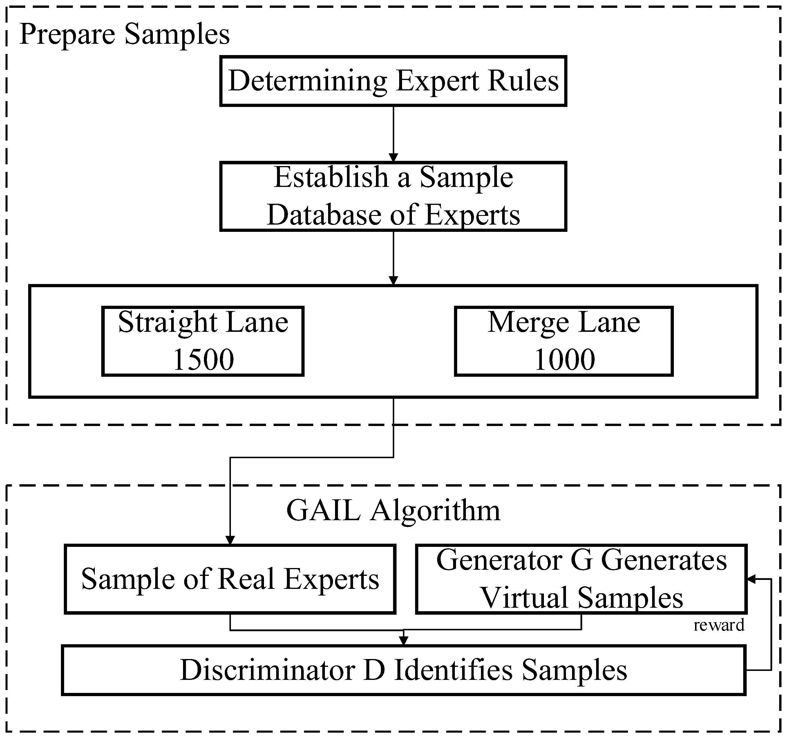
2.4.5. Sample Build Process

Based on the above expert rule base, the vehicle decision-making model is trained in the simulation scene, and the expert sample base is constructed. As shown in Figure 5, a total of 1500 pieces of sample data are collected for the straight lane scene, and 1000 pieces of sample data are collected for the merge lane scene.

2.5. The Pseudo-Code of Algorithm

The pseudo-code of DGAIL algorithm is shown in

Table 2. DGAIL algorithm pseudo-code.

Serial	DGAIL Algorithm Pseudo-Code
1:	Initialize replay memory D to capacity N;
2:	Initialize the network weight η of discriminator D;
3:	For i = 1, N do(i is the total number of training rounds):
4:	For j = 1, M do(j is the number of iterations for each training round):
5:	The input state is st at time t, Action at is selected by the ε-greedy strategy;
6:	The agent performs action a and obtains state st+1 at time t + 1;
7:	END For
8:	The false sample set (st, at) of the agent is obtained;
9:	Discretize the expert sample χ to obtain the expert sample set (expert_st, expert_at);
10:	Input the fake sample set (st, at) and expert sample set (expert_st,  expert_at) into the discriminator D;
11:	Discriminator D receives expert sample data and fake sample data;
12:	REPEAT (5 times):
13:	Discriminator D uses the gradient descent method to train the loss   function, updates the weight η of the neural network, judges the   authenticity of the sample, and outputs the reward value function rt;
14:	Recombine (st, at, rt, and st+1) and store it in the experience pool D of generator G;
15:	Update the weights θ of the generator G estimation network and target  network to complete one round of training;
16:	END For

.

3. Simulation Test and Results

Several numerical simulations are conducted to demonstrate the efficacy of our proposed algorithm. The straight road scene and merging road scene are selected to verify the algorithm in the simulation. The purpose is to test whether the algorithm has the ability to complete safe driving within the specified time and compare the effects of different algorithms. The experimental simulation environment is as follows: operating system is WIN10 operating system, CPU is Inter Core i7-7700 processor, memory is 8 GB, GPU is NVIDIA GeForce GTX 1060, programming language is Python, and deep learning tool is Pytorch.

3.1. Simulation Parameter Settings

3.1.1. Straight Road Scene

The straight road scene is a one-way three-lane scene with a total lane length of 1000 m. The state space S includes the location information and motion information of the surrounding five vehicles. The vehicles in this scenario are available for free, random actions. The parameters of the specific environment model are shown in

Table 3. Straight road scene environmental model parameters.

Parameter	Description	Value
Lane_length	Road length/m	1200
Lane_width	Single lane width/m	3.6
Lane_number	Number of lanes	3
Length	Vehicle length/m	5
Width	Vehicle width/m	2
Acc	Max acceleration/(m/s2)	6
Dec	Max deceleration/(m/s2)	5
V_max	Maximum lane speed limit/(m/s)	30
V_min	Minimum lane speed limit/(m/s)	20
Vehice_number	Number of vehicles	10
Frequency	Environment refresh cycle/s	0.1

.

3.1.2. Merging Road Scene

The merging road scene is a one-way two-lane scene that includes an outer ramp, and the total length is 400 m. The state space S includes the location information and motion information of the surrounding five vehicles. The vehicles in this scenario are available for free, random actions. The parameters of the specific environmental model are shown in

Table 4. Merging road scene environmental model parameters.

Parameter	Description	Value
Lane_length	Road length/m	500
Lane_width	Single lane width/m	3.6
Lane_number	Number of lanes	3
Length	Vehicle length/m	5
Width	Vehicle width/m	2
Acc	Max acceleration/(m/s2)	6
Dec	Max deceleration/(m/s2)	5
V_max	Maximum lane speed limit/(m/s)	30
V_min	Minimum lane speed limit/(m/s)	20
Vehice_number	Number of vehicles	7
Frequency	Environment refresh cycle/s	0.1

.

3.1.3. Action Space Settings

Vehicle action space includes acceleration, left lane change, right lane change and follow ahead.

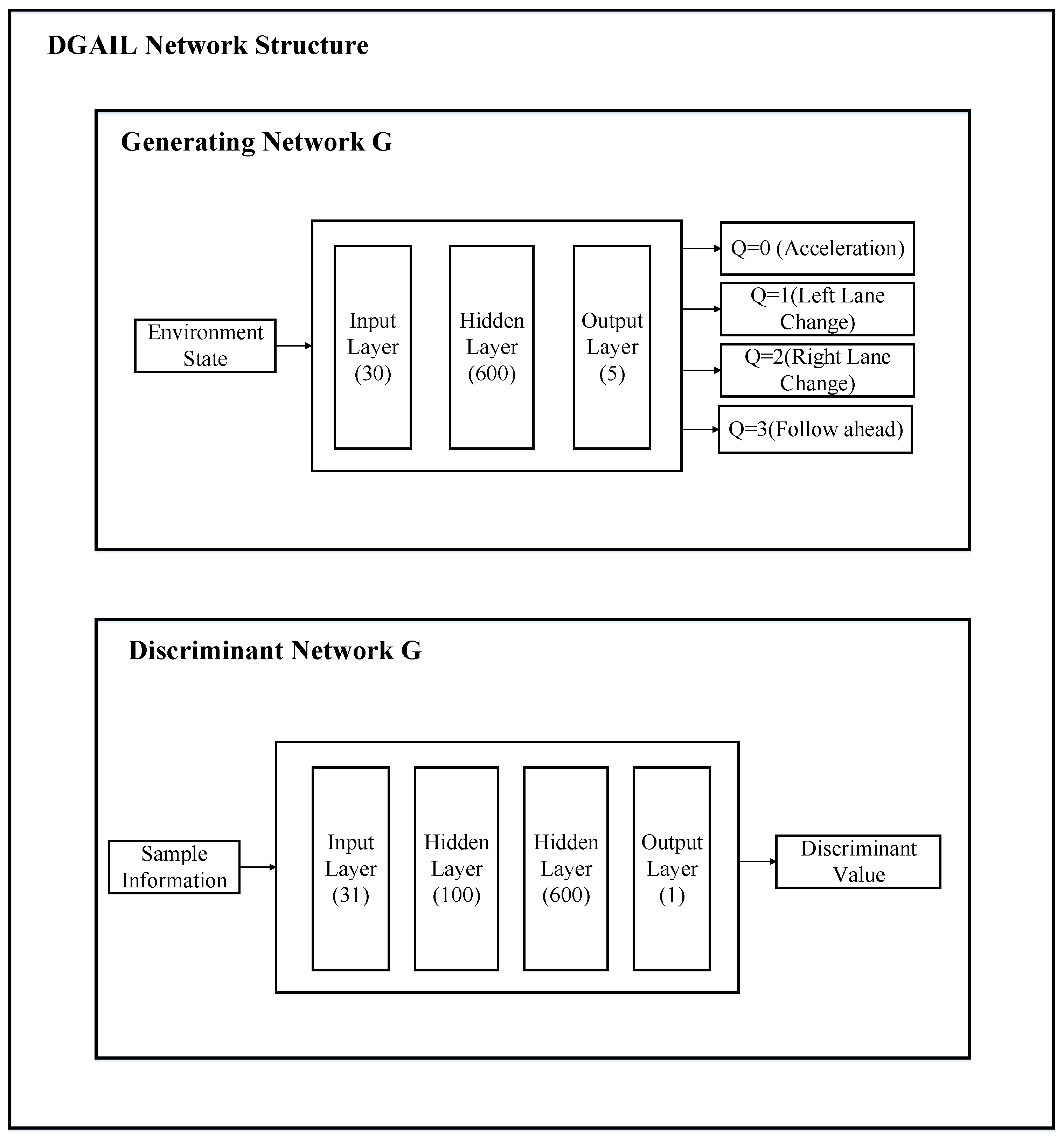
3.1.4. Neural Network Parameter Settings

The value network and target network are structured by BP neural network, in which the hidden layer consists of 600 neurons. The Leaky-Relu activation function is used between the input and hidden layers and between the hidden and output layers. The specific structure is shown in Figure 6.

3.2. DGAIL Algorithm Simulation Results Analysis

In order to test the simulation effect in two scenarios, we train the decision-making model in the traffic simulation platform with the DGAIL algorithm. When the model converges to stability, the motion of the vehicle is as shown in Figure 7, in which the green square represents the main vehicle and the blue square represents the environment vehicles.

• Straight Road Scene

Figure 7. The driving state of vehicle on the straight road.

Figure 7. The driving state of vehicle on the straight road.

As shown in Figure 7a is the environmental state at the initial moment, including one ego-vehicle and 10 environmental vehicles, and (b–h) is the vehicle driving process. At the initial moment (a), the ego-vehicle is located in the middle lane, the longitudinal displacement is 0 m, and the initial speed is 25 m/s; at the moment (b), as the vehicle ahead enters the minimum safe distance, the ego-vehicle changes lane left to overtake at a speed of 25 m/s; at the moment (c), the ego-vehicle keeps going straight and accelerates to 30 m/s; at the moment (d), due to two obstacle vehicles ahead and no space for lane change, the ego-vehicle slows down to follow the vehicle ahead and decelerates to 20 m/s; at the moment (e), the ego-vehicle changes lane right to overtake and maintains its speed at 20 m/s; at the moment (f), the ego-vehicle continues going straight and accelerates to 25 m/s; at the moment (g), as the vehicle ahead enters the minimum safe distance, the ego-vehicle changes lane left to overtake at a speed of 25 m/s; at the moment (h), the ego-vehicle keeps going straight and accelerates to 30 m/s until the end of this trip.

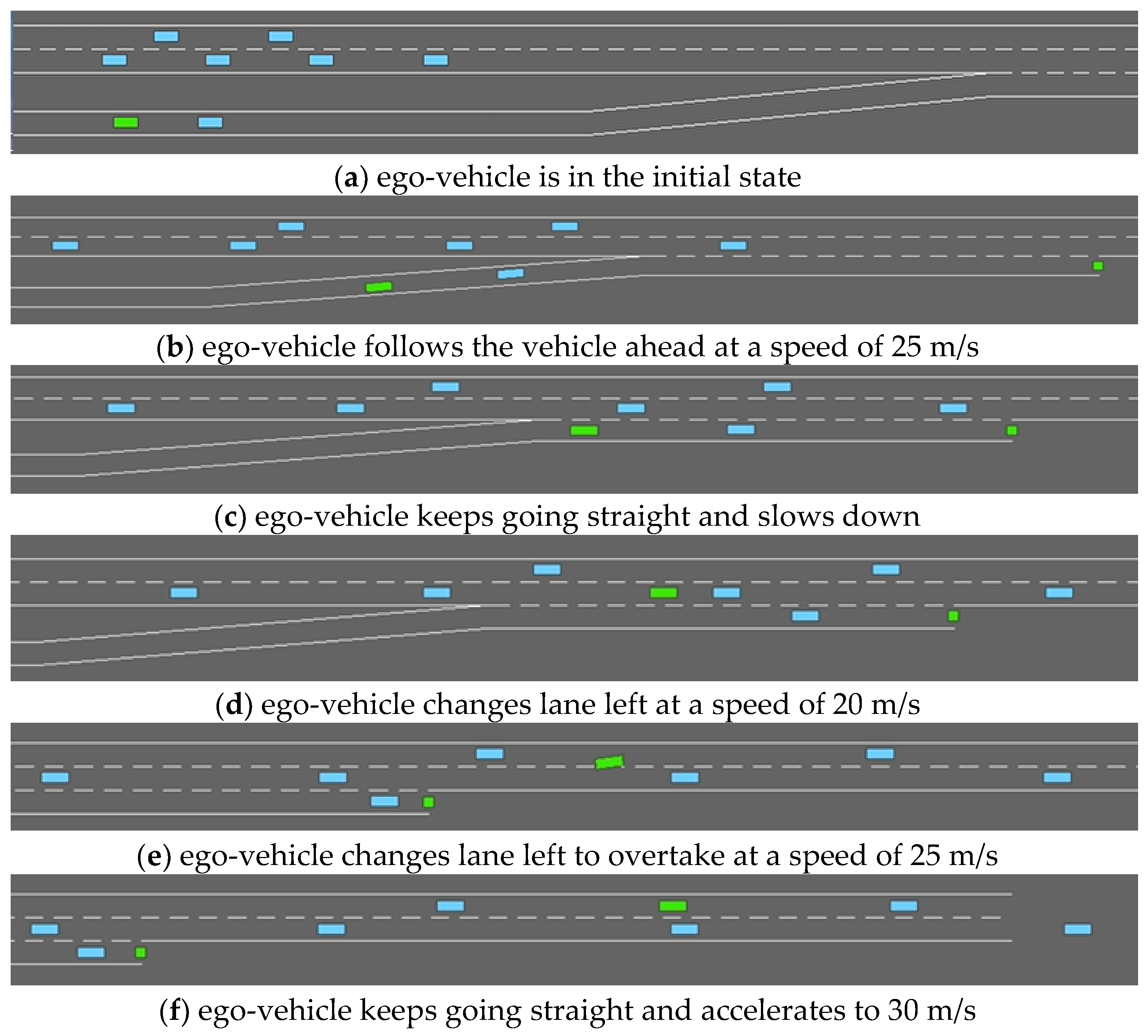
• Merging Road Scene

As shown in Figure 8a is the environmental state at the initial moment, including one ego-vehicle and seven environmental vehicles, and (b–f) is the vehicle driving process. At the initial moment (a), the ego-vehicle is located in the middle lane, the longitudinal displacement is 0 m, and the initial speed is 25 m/s; at the moment (b), the ego-vehicle keeps a safe distance to follow the vehicle ahead at a speed of 25 m/s; at the moment (c), the ego-vehicle keeps going straight and slows down to wait for the left lane to be vacated, and the speed of the ego-vehicle drops to 20 m/s; at the moment (d), as the left lane is vacant, the ego-vehicle changes lane left at a speed of 20 m/s; at the moment (e), as the vehicle ahead enters the minimum safe distance, the ego-vehicle changes lane left to overtake at a speed of 25 m/s; at the moment (f), the ego-vehicle keeps going straight and accelerates to 30 m/s until the end of this trip.

4. Discussion

4.1. Straight Road Scene

4.1.1. Training Convergence

As shown in Figure 9, according to the established training parameters, in the 0–750 rounds, the decision-making model had high randomness in the selection of actions, and the neural network had not yet converged. In the 750–1600 rounds, the vehicle driving time and reward value gradually increased as the loss function of the value network began to converge. In the 1600–2000 rounds, the driving time of the vehicle was reached and stabilized at 40 s, the training task of the straight road scene was completed, and the reward value gradually converged and stabilized at 35.5.

4.1.2. Training Time Cost

The training time cost refers to the number of training rounds used by the learning model to achieve convergence in training. Combined with the training process of the driving behavior decision-making model, the round duration, reward value, and training times were selected as the training time cost indicators of the decision-making model, and the DQN, GAIL, A3C and DGAIL methods were applied to complete the test of the straight road scene. The results are shown in

Table 5. Training time cost for straight road.

Algorithm	Reward Value	Round Duration	Training Times
DQN	30.8	24	2231
GAIL	5.2	24	3000
A3C	32.3	40	1853
DGAIL	35.5	40	1651

. The DGAIL method only used 1470 times to achieve convergence, with the fewest training times and the highest reward value. The A3C method achieved convergence after 1853 iterations, with the same training time and 2nd reward value. The DQN method achieved convergence after 2231 iterations, with the same training time and 3rd reward value. The GAIL could not complete the training in 3000 training times.

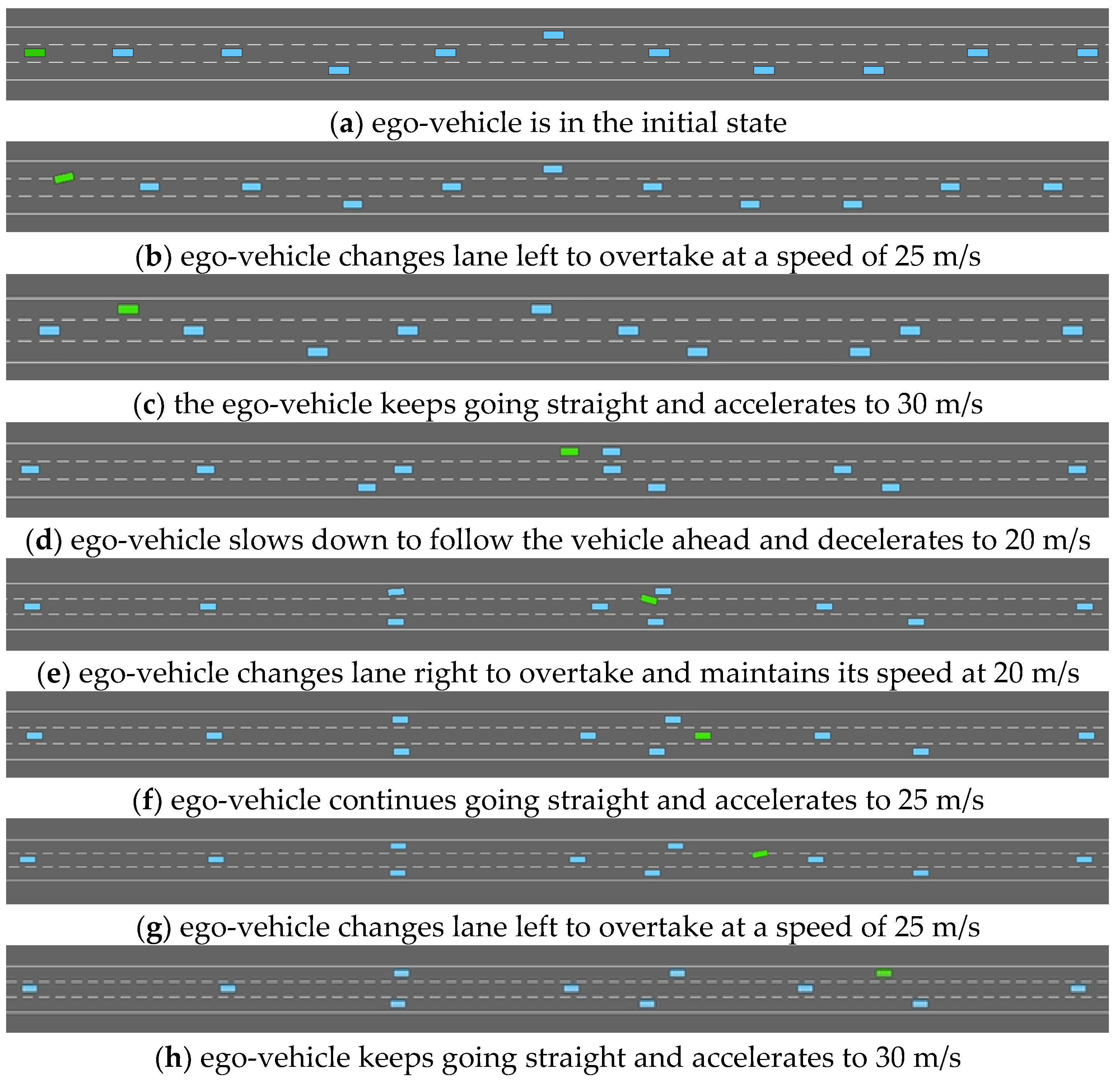
4.1.3. Effectiveness of Driving Strategies

Comparison of decision-making model based on DGAIL and A3C in the same simulation scenes and parameter settings. The training results and vehicle motion parameter curves of the two different algorithms for the vehicle in the straight road scene during simulation progress are shown in Figure 10 and Figure 11.

As shown in Figure 10, in the 1000 rounds, both algorithms were in the initial learning stage, and the decision-making model had high randomness in the selection of actions. In the 1000–1600 rounds, the DGAIL algorithm started to make correct decisions based on expert knowledge, and the success rate increased rapidly to 94% and the reward value increased to 32.25. In contrast, the A3C algorithm was still in the exploration stage, during which the randomness of the action selection strategy was larger, and the success rate and reward value were lower. In the 1600–1800 rounds, the DGAIL algorithm continued to learn the empirical knowledge that was generated from the interaction with the environment, the decision-making model was approaching the expert level, and the success rate and reward value were in the stable rising stage. At this time, the A3C algorithm also began to learn the correct action decision, the randomness of the action selection strategy was reduced, and the success rate and reward value continued to rise. In the 1800–2000 rounds, both algorithms had learned the optimal strategy, the decision-making model entered a stable period, and the driving decision obtained was able to meet the needs of the straight road scene. As shown in Figure 11, compared with the A3C algorithm, the DGAIL algorithm had a slightly higher average vehicle speed, fewer lane changes, more frequent acceleration and deceleration, and higher total rewards value considering the influence of the reward guidance factor.

4.2. Merging Road Scene

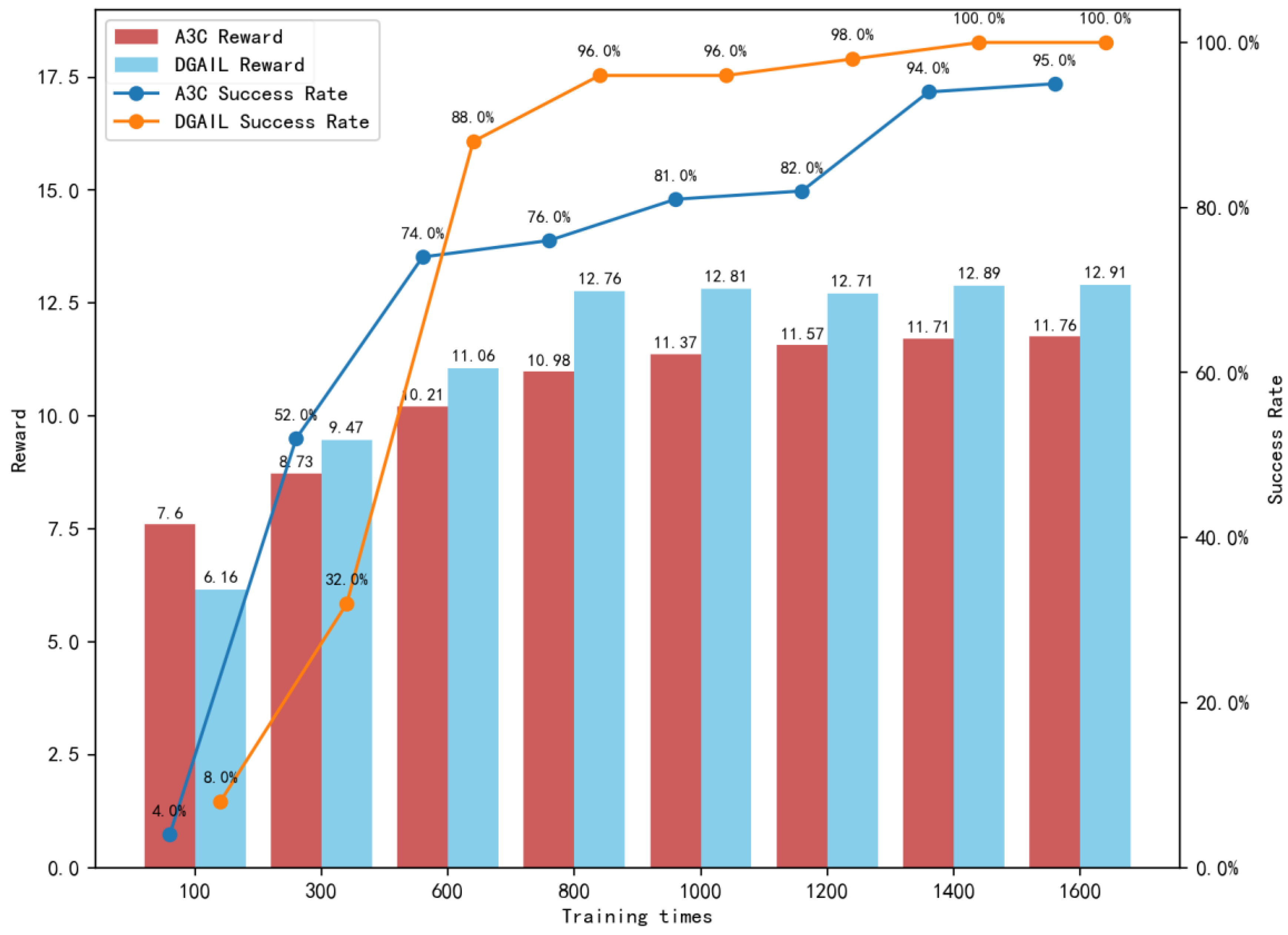
4.2.1. Training Convergence

As shown in Figure 12, according to the established training parameters, in the 0–400 rounds, the decision-making model had high randomness in the selection of actions, and the neural network had not yet converged. In the 400–750 rounds, the vehicle driving time and reward value gradually increased as the loss function of the network began to converge. In the 750–2000 rounds, the ego-vehicle’s travel time was stable at 15 s, reward value gradually converged at 13.8, and the training task of the merging road scene was completed.

4.2.2. Training Time Cost

Combined with the training process of the driving behavior decision-making model, the round duration, reward value, and training times were selected as the training time cost indicators of the decision-making model, and the DQN, GAIL, A3C and DGAIL methods were applied to complete the test of the merging road scene. The results are shown in

Table 6. Training time cost for merging road.

Algorithm	Reward Value	Round Duration	Training Times
DQN	9.5	11	1782
GAIL	4.8	11	2000
A3C	11.76	15	1189
DGAIL	12.9	15	855

. The DGAIL method only used 1075 times to achieve convergence, with the fewest training times and the highest reward value. The A3C method achieved convergence after 1312 iterations, with the same training time and second-highest reward value. The DQN method achieved convergence after 1782 iterations, with the same training time and third-highest reward value. The GAIL could not complete the training in 2000 training times.

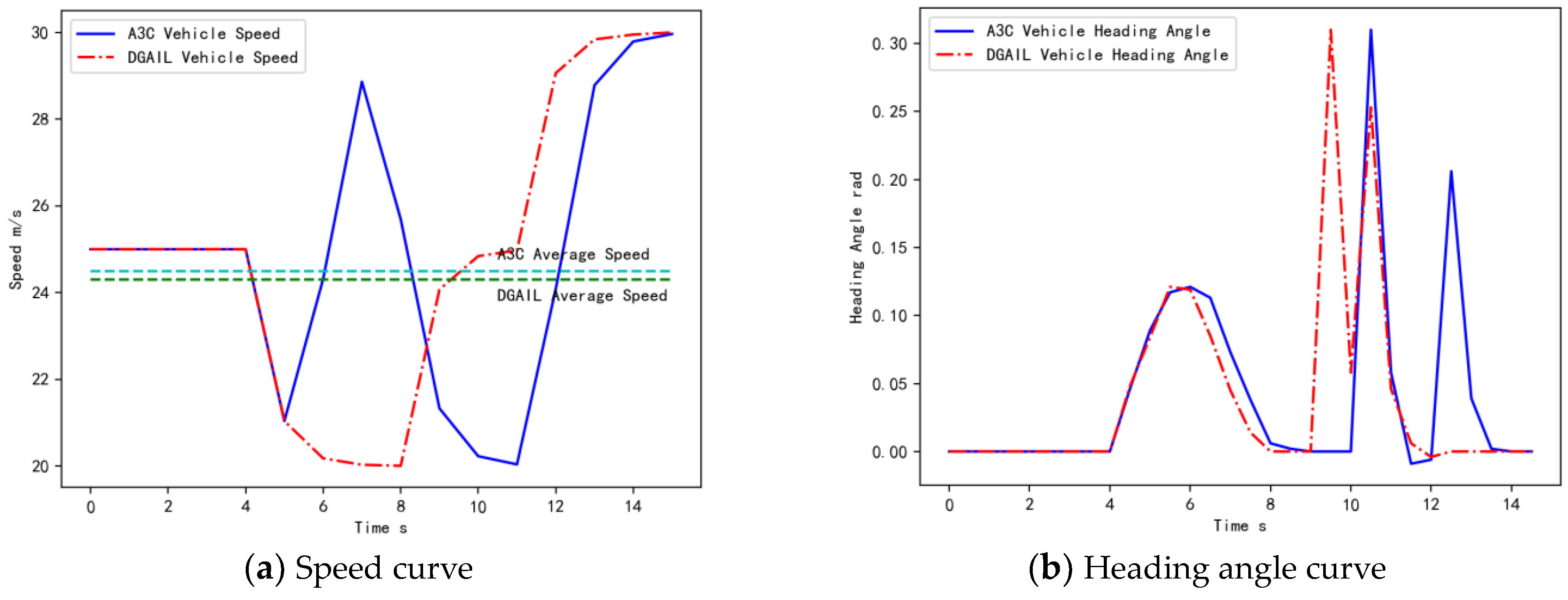
4.2.3. Effectiveness of Driving Strategies

Comparison of decision-making model was based on DGAIL and A3C in the same simulation scenes and parameter settings. The training results and vehicle motion parameter curves of the two different algorithms for the vehicle in the merging road scene during simulation progress are shown in Figure 13 and Figure 14.

As show in Figure 13, in the 300 rounds, both algorithms were in the initial learning stage, and the decision-making model had high randomness in the selection of actions. In the 300–800 rounds, the DGAIL algorithm started to make correct decisions based on expert knowledge, the success rate increased rapidly to 96%, and the reward value increased to 12.76. In contrast, the A3C algorithm was still in the exploration stage; the randomness of the action selection strategy was larger, and the success rate and reward value were lower. In the 800–1200 rounds, the DGAIL algorithm continued to learn the empirical knowledge that was generated from the interaction with the environment, the decision-making model was approaching the expert level, and the success rate and reward value were in the stable rising stage. At this time, the A3C algorithm also began to learn the correct action decision, the randomness of the action selection strategy was reduced, and the success rate and reward value continued to rise. In the 1200–1600 rounds, both algorithms had learned the optimal strategy, the decision-making model entered a stable period, and the driving decision obtained was able to meet the needs of the straight road scene. As shown in Figure 14, compared with the A3C algorithm, the DGAIL algorithm had a slightly higher average vehicle speed, fewer lane changes, more frequent acceleration and deceleration, and higher total rewards value considering the influence of the reward guidance factor.

5. Conclusions

Relying on relevant scientific research projects, this paper treated intelligent vehicles as the research object and analyzed the decision-making method for vehicle driving behavior. First, the development and related algorithms of intelligent vehicle behavior decision-making were introduced. Second, the DQN algorithm was used to optimize the GAIL algorithm, and the DGAIL algorithm was proposed. In addition, a vehicle decision-making model based on DGAIL was constructed, including the design of the state space, design of the network structure and design of the training parameters. Last, in a typical scenario, the training and verification in the simulation scenario were completed according to the vehicle decision model. The results show that the algorithm meets the requirements of intelligent vehicles for decision-making systems. Core innovations include the following:

• A DGAIL-based intelligent vehicle driving behavior decision-making method, which can realize real-time, reliable, and stable decision-making in traffic scenarios based on structured roads, is proposed. Compared with the deep reinforcement learning DQN method, the tedious design of the reward value function is omitted. Compared with the traditional GAIL method, the DGAIL method is more suitable for scenes where the action space is discrete, the training convergence is faster, and the stability is higher.
• Presently, most research on intelligent vehicle driving behavior decision-making is mainly aimed at straight roads and intersections. In this paper, by constructing merging and roundabout scenarios in the simulation environment, the research scenarios of intelligent vehicles are enriched, and the decision-making of intelligent vehicle driving behavior can be more comprehensively verified. The applicability of the method accelerates the research process of a deep reinforcement learning algorithm in driving behavior decision-making.
• By proposing the DGAIL method, the effectiveness of generative adversarial imitation learning in structured scenarios is evaluated and then trained and validated in traffic simulation scenarios. However, there are still some deficiencies in this paper in some aspects. Further research and exploration can be carried out from the following aspects:
• The complexity of the scene: Although the scene in this paper included straight road and merging scenes, there were still certain constraints on the environmental vehicles in it, and the complexity was relatively simple. The driving behavior of smart cars in more free scenes can be explored in future studies.
• Optimization of the DGAIL algorithm: Although the DGAIL algorithm omits the design process of the reward value function, its training results have no obvious advantages over the traditional DQN algorithm. In follow-up research, the structure of the DGAIL algorithm can be optimized to improve the effectiveness and stability of the algorithm.
• Real vehicle test: The research in this paper was completely based on simulation and is still far from real practical use. In future studies, the algorithm in the simulation can be extended to real scenes through transfer learning, and the effectiveness of the method can be further demonstrated from an actual environment.

References

- State Council of the PRC. Made in China 2025. Available online: http://www.gov.cn/zhengce/zhengceku/2015-05/19/content_9784.htm (accessed on 12 September 2022).
- Li, F. Research and Evaluation on Comprehensive Obstacle-Avoiding Behavior for Unmanned Vehicles; Beijing Institute of Technology: Beijing, China, 2015. [Google Scholar]
- Chae, H.; Kang, C.M.; Kim, B.D.; Kim, J.; Chung, C.C.; Choi, J.W. Autonomous braking system via deep reinforcement learning. In Proceedings of the 2017 IEEE 20th International Conference on Intelligent Transportation Systems (ITSC), Yokohama, Japan, 16–19 October 2017; pp. 1–6. [Google Scholar]
- Jaritz, M.; De Charette, R.; Toromanoff, M.; Perot, E.; Nashashibi, F. End-to-end race driving with deep reinforcement learning. In Proceedings of the 2018 IEEE International Conference on Robotics and Automation (ICRA), Brisbane, Australia, 21–25 May 2018; pp. 2070–2075. [Google Scholar]
- Kendall, A.; Hawke, J.; Janz, D.; Mazur, P.; Reda, D.; Allen, J.M.; Lam, V.D.; Bewley, A.; Shah, A. Learning to drive in a day. In Proceedings of the 2019 International Conference on Robotics and Automation (ICRA), Montreal, QC, Canada, 20–24 May 2019; pp. 8248–8254. [Google Scholar]
- Fang, C. Research of the Lane Following Decision-making of Autonomous Vehicle Based on Deep Reinforcement Learning. Master Thesis, Nanjing University, Nanjing, China, 2019. [Google Scholar]
- Alizadeh, A.; Moghadam, M.; Bicer, Y.; Ure, N.K.; Yavas, U.; Kurtulus, C. Automated lane change decision making using deep reinforcement learning in dynamic and uncertain highway environment. In Proceedings of the 2019 IEEE Intelligent Transportation Systems Conference (ITSC), Auckland, New Zealand, 27–30 October 2019; pp. 1399–1404. [Google Scholar]
- Luo, P.; Huang, Z.; Qing, Y.; Chen, Z. A method of vehicle driving behavior decision based on DQN algorithm. J. Transp. Inf. Saf. 2020, 38, 67–77, 112. [Google Scholar]
- Kober, J.; Peters, J. Imitation and reinforcement learning. IEEE Robot. Autom. Mag. 2010, 17, 55–62. [Google Scholar] [CrossRef]
- Ho, J.; Ermon, S. Generative adversarial imitation learning. arXiv 2016, arXiv:1606.03476. [Google Scholar]
- Hausman, K.; Chebotar, Y.; Schaal, S.; Sukhatme, G.; Lim, J.J. Multi-modal imitation learning from unstructured demonstrations using generative adversarial nets. arXiv 2017, arXiv:1705.10479. [Google Scholar]
- Merel, J.; Tassa, Y.; Dhruva, T.B.; Srinivasan, S.; Lemmon, J.; Wang, Z.; Wayne, G.; Heess, N. Learning human behaviors from motion capture by adversarial imitation. arXiv 2017, arXiv:1707.02201. [Google Scholar]
- Li, Y.; Song, J.; Ermon, S. Infogail: Interpretable imitation learning from visual demonstrations. arXiv 2017, arXiv:1703.08840. [Google Scholar]
- Song, J.; Ren, H.; Sadigh, D.; Ermon, S. Multi-agent generative adversarial imitation learning. arXiv 2018, arXiv:1807.09936. [Google Scholar]
- Schulman, J.; Levine, S.; Abbeel, P.; Jordan, M.; Moritz, P. Trust region policy optimization. In Proceedings of the International Conference on Machine Learning, Lille, France, 7–9 July 2015; pp. 1889–1897. [Google Scholar]
- Schulman, J.; Wolski, F.; Dhariwal, P.; Radford, A.; Klimov, O. Proximal policy optimization algorithms. arXiv 2017, arXiv:1707.06347. [Google Scholar]
- Goodfellow, I.; Pouget-Abadie, J.; Mirza, M.; Xu, B.; Warde-Farley, D.; Ozair, S.; Courville, A.; Bengio, Y. Generative adversarial networks. Commun. ACM 2020, 63, 139–144. [Google Scholar] [CrossRef]