A Study on the Optimization of the Coil Defect Detection Model Based on Deep Learning

Abstract

With increasing interest in smart factories, considerable attention has been paid to the development of deep-learning-based quality inspection systems. Deep-learning-based quality inspection helps productivity improvements by solving the limitations of existing quality inspection methods (e.g., an inspector’s human errors, various defects, and so on). In this study, we propose an optimized YOLO (You Only Look Once) v5-based model for inspecting small coils. Performance improvement techniques (model structure modification, model scaling, pruning) are applied for model optimization. Furthermore, the model is prepared by adding data applied with histogram equalization to improve model performance. Compared with the base model, the proposed YOLOv5 model takes nearly half the time for coil inspection and improves the accuracy of inspection by up to approximately 1.6%, thereby enhancing the reliability and productivity of the final products.

1. Introduction

A quality inspection system is used for obtaining consistent quality results at manufacturing sites. Quality inspection systems afford advantages such as product quality improvements and solutions to labor shortages to companies. However, existing quality inspection systems may differ in inspection performance because of the fatigue and different skill levels of human inspectors due to a rule- or visual-based inspection. In the present study, one surface of a coil—an inspection target—is inspected as shown in Figure 1A. Approximately 1–1.5 s are required for an inspector to inspect around 10 coils (Figure 1B). According to Figure 1B, the inspector inspects only one side during the inspection time. In addition, Taiwan’s inspectors must take a certain amount of time off during working hours.

To consistently maintain the performance of quality inspection systems and reduce human errors, deep-learning-based machine vision technology has been applied in quality inspection, and related studies have been actively conducted. With the Fourth Industrial Revolution, considerable attention has been paid to artificial intelligence (AI) and recognition technologies based on AI have greatly advanced. As significant attention has been paid to AI technology even at manufacturing sites, several studies on the application of intelligent machine vision technologies to quality inspection systems have been conducted [1,2].

Machine vision technology using deep learning shows a performance of about 95% when evaluated by mAP, and is used in various fields [3,4,5]. The machine vision market is also projected to witness tremendous growth in the future. As depicted in Figure 2A, the global machine vision market will grow at approximately 7% annually, resulting in a market of around USD 15.5 billion by 2026. In particular, hardware and software markets in machine vision will grow at approximately 6% and 10.3%, which will be worth around USD 11.3 billion and 4 billion, respectively, as shown in Figure 2B.

In this study, a quality inspection system based on deep learning technology is proposed. YOLOv5 is a model of the YOLO family, a real-time object detection model, that can find desired objects in a short time [7]. In this study, model optimization for defect detection of small objects is carried out using the YOLO family of models. Various model performance improvement techniques are used to analyze the impact on model performance, and model optimization is carried out based on the results. In addition, additional model optimization is carried out by adding data that has undergone image preprocessing to effectively extract the features of the image.

Related works associated with this can be found in Section 2. In Section 3, the proposed quality inspection system is explained and a model using the system and various performance improvement techniques for the model (algorithm structure optimization, model scaling, and light weight) are analyzed. In Section 4, the results of the performance improvement techniques, which are applied to the model, are comparatively analyzed to propose the optimum model of the intelligent machine vision inspection system.

2. Related Research

Studies have been conducted on methods to improve model performance, such as modifying a model structure or combining a model with other models to reduce computation and improve inference speed. Using the YOLO family model, we analyzed performance improvement studies with model and dataset modifications.

In order to improve model performance, the main method is to modify the existing model using other models. This can be confirmed through the following studies. Alivek et al. [8] used the EfficientNet model to classify defects in advance, and based on this result the YOLOv5 model was used to indicate the location of defects. Kim et al. [9] used two YOLO algorithm versions to detect microscopic images of defects that were discovered in the process and conducted a comparative analysis of their performance. In their study, YOLOv3 and YOLOv5s models were used. They found that the YOLOv5s model exhibited better inference speed with a relatively small weight capacity than that of the YOLOv3 model, and the mean average precision was around 1% higher as well. Zhao et al. [10] applied the GhostBottlenet module instead of using the backbone’s Conv module in the existing YOLOv5 model to reduce the network computation by compressing the parameters in the YOLOv5 model and increase the model’s inference speed. The GhostBottlenet module reduced the computation by approximately 36% compared with that of the YOLOv5s model and improved performance by approximately 2%. Usamentiaga et al. [11] applied a deep-learning-based machine vision inspection system to detect surface defects in steel. Here, YOLOv5 and U-Net, representative computer vision algorithms, were applied to the study. The applicability of a deep-learning-based machine vision inspection system was demonstrated by showing high-level defect detection results.

In addition, methods are being studied to improve model performance by solving problems arising from unbalanced or small amounts of data. To resolve these problems, a study using data augmentation, feature extraction, and noise removal was conducted as follows: Yun et al. [12] augmented an amount of data using an autoencoder to solve the data imbalance that occurred in defect detection and verified the performance improvement through experiments. In addition, Feng et al. [13] also described the performance differences according to various versions of YOLOv5 and data augmentation. The larger the size of the model and the more datasets used for learning, the longer the learning time was, but the performance tended to improve. The unique characteristics vary according to the inspection target. Thus, techniques that can well extract the characteristics of the target should be applied. Wang et al. [14] aimed to easily extract defects of the inspection target using the region of interest and Hough transform techniques.

Analyzing the above research trends, there are various methods of using the model according to the purpose and direction of the study. This process depends on the purpose and direction of each study, and the performance of the model also varies. Therefore, it is important to implement an appropriate model by utilizing high-quality datasets. Based on the preceding studies, the present study attempted to improve the model performance from the data and the model viewpoint to enhance the performance of the existing YOLOv5 model. To improve the model performance, image data upgraded through the histogram equalization of datasets and performance-enhancement techniques such as structure modification, model scaling, and a lightweight model design are used. Unlike previous studies, this study does not present only differences from existing models. Various techniques for improving performance are applied and the results are analyzed. Trends are analyzed through result analysis, and the impact on performance is analyzed. Based on this, we present a model optimized for small object detection.

3. Methodology

This section describes the system to which the model proposed in this study is applied. In addition, we describe the YOLOv5 model and the techniques and datasets applied in this study to improve the performance of the model. The proposed YOLOv5 model utilizes an image dataset collected through a prototype to conduct model training. Thereafter, in order to apply the performance improvement technique and the image preprocessing technique, the optimal parameter value suitable for this study is found, and model training is conducted by applying it to the YOLOv5 model.

The following Figure 3 is a diagram of the system to which the model proposed in this study is applied. The coil is photographed using a camera and defect detection is carried out through a model that suggests it. The detection results are visualized through the bounding box and the results of the detection are expressed as probabilities.

3.1. System Overview

The inspection target of the proposed system is a small part that uses a reel as shown in Figure 4C. Condensers, resistors, diodes, and power coils are some examples of such targets. In this study, a coil is selected as the inspection target.

Figure 4A shows the overall structure of the trial product that performs inspections as the system is applied, and Figure 4B shows the detailed images of the main components in the trial product such as the camera, lens, and light. The overall process of the coil defect detection system is as follows: A coil, which is an inspection target, is inserted into the equipment, in which the camera and light are installed through the rail. The inserted coil is photographed through the camera equipment, and the system determines whether the photographed coil is normal or defective through the trained model. The dataset for training the deep learning model used in this study is also created using the trial product.

3.2. YOLOv5 Model and Performance Improvement Techniques

This section describes the deep learning model used in the study and the techniques applied to the YOLO model for model optimization. In addition, the image pre-processing technique applied to the dataset of this study and the image quality evaluation technique utilized for the application of appropriate hyperparameters are also described.

3.2.1. YOLO

YOLO is a universal object detection algorithm focusing on fast inference speed, as the localization and classification of the object in the image or video are conducted simultaneously in the object detection process. To date, various versions of YOLO models have been released through continuous performance improvements. Figure 5 shows the structure of YOLOv5 [15], which is used in the present study.

The backbone of YOLOv5 is mainly composed of a single block called Conv, which includes three components (convolution, batch normalization, and leaky ReLu), a C3 block that employs CSPNet [16], and the spatial pyramid pooling (SPP) algorithm. Conv blocks consist of convolution, batch normalization, and activation functions, and in this study, Conv blocks are added for performance analysis through structural modifications. This structural modification is intended to analyze the effect of more feature map extraction on the performance of the model. The purpose of CSPNet is to reduce the computation increase due to the duplication of the weight information created during the learning process. In a partial dense block, the feature maps are split into two parts: one part goes through a dense block and the other part is directly linked to the end of the stage as shown in Figure 6. In a partial transition layer, the concatenation of the output through the dense block and the output that is directly linked to the end of the stage is used as the input value. This process can be effective in reducing duplicate weights as well as computation.

Existing CNN models have input size limitations due to fully connected layers. However, SPPNet [17] tried to solve the problems that could arise by removing the input size limit. The feature map extracted through the convolution layer is divided into a predetermined bin. After that, max pooling is applied to the bin, and then the results are connected. Through this, it is possible to extract an output value of a certain size regardless of the image size.

In the Neck, a block used in the backbone is applied to a path aggregation network (PAN) [18] to improve the performance. PAN allows improved performance by further adding a bottom-up path to the feature pyramid network [19]. It aims to transfer a feature in the bottom hierarchy to the top hierarchy because the feature from the bottom hierarchy is less influential up to the last hierarchy.

Finally, the Head extracts the results for three different sizes, the same as in YOLOv3 [20], and aims to detect objects with various sizes in an image or video.

To improve the model performance, model scaling that generally adjusts the model’s depth and width as well as the input image size can be performed. Further, five different YOLOv5 models are proposed through model scaling as shown in Figure 7.

Table 1. Scale ratios of YOLOv5 models.

Name	Depth	Width
YOLOv5x	1.33	1.25
YOLOv5l	1.00	1.00
YOLOv5m	0.67	0.75
YOLOv5s	0.33	0.50
YOLOv5n	0.33	0.25

presents the model scale ratio in five different versions, which are categorized as “XLarge,” “Large,” “Medium,” “Small,” and “Nano.”

The model scaling value becomes large from Nano to XLarge. As verified in Figure 8, mAP values improve as the model scaling value becomes larger; however, the inference time is slower and the capacity of the final model also increases. The present study aims to improve the model performance by changing the model scaling value to find the optimum model.

3.2.2. Performance Improvement Techniques

A lightweight model is an important element in a deep-learning-based system. General deep learning systems require high-performance computing capabilities. However, implementing high-performance computing using equipment and robots used on sites is difficult. Thus, a lightweight model that exhibits comparable performance is required, and numerous related studies have been conducted accordingly. A lightweight model is also required in the proposed system. Accordingly, we explain some of the typical techniques for a lightweight model, such as knowledge distillation and quantization, as well as pruning, which is used in this study.

Knowledge distillation [21] is a technique devised to create a smaller model from ensembles of many models that are already trained. This technique reduces the storage space where the model is stored and execution memory usage by obtaining a smaller model with fewer training parameters and a smaller bit width based on previously trained models considering the performance limitation in embedded devices.

Quantization [22] is a technique to represent 32-bit floating point (FP32)-based learning parameters with a 1K-bit size, which is a smaller-bit-width integer than that of FP32-based learning parameters. In many cases, deep learning models mainly use the FP32 type to store parameters generated after training, which affords the advantage that the model size could be theoretically reduced by 32/K times without discarding some parameters. However, it may cause accuracy loss because the range of numbers that could be represented is significantly limited owing to smaller-bit-width integers.

Finally, pruning [23] (Figure 8) is a technique based on the viewpoint that “not all parameters have the same effect on inference.” It is a lightweight technique that removes neurons and layers that do not significantly influence the inference process while learning iteratively, thereby obtaining a model whose parameters are considerably reduced. Pruning is used in the present study to optimize the model. We attempted to lighten the model by spinning the Conv block, which occupies the most parameters in the model of YOLOv5.

3.3. Dataset

The dataset created through the trial product contained around 13,000 images, which are divided into 9500 images in the dataset for learning, 2500 images for validation, and finally 1000 images for the dataset for testing. The classes in the datasets for classification are divided into four groups: ‘T-OK’, ‘T-NG’, ‘OK’, and ‘NG’. The reason for creating four classes is because the left and right sides had the same appearance except for the top side when we shot the coil from three directions (top, left, and right) as shown in Figure 9. Thus, four classes are set to distinguish normal and defective cases in the top, normal, and defective cases in the left and right.

Figure 10 shows the defective cases on the top, left, and right sides. The defect in the top is defined as the coil wire being broken or deformed in the area indicated in the image. The defect in the left and right is defined as the upper and lower plates being misaligned as shown in the two boxes in the image.

3.4. Preprocessing of Images

This section describes the preprocessing technique applied to the dataset of this study and describes the quality evaluation technique used to find appropriate parameter values.

3.4.1. Contrast-Limited Adaptive Histogram Equalization

We attempted effective feature extraction through the contrast change because coil data are black-and-white images and we aimed to enhance contrast changes through histogram equalization (HE). However, HE has a drawback of noise increase when a part of the image to be applied has a distribution different from that of other parts. The Contrast-Limited Adaptive Histogram Equalization (CLAHE) used in this study is a method proposed to overcome the drawback of HE. It is an equalization method to prevent excessive amplification of contrast during the equalization process of an image or video and maintains characteristics similar to those of the original.

The input image is divided into grids of the same size and CLAHE is conducted in each divided grid as shown in Figure 11. The applied result is shown in Figure 12A,B. Figure 13 shows HE- and CLAHE-applied histograms to coil images, which verifies that the histogram of CLAHE is more similar to the original histogram than that of HE when equalization is conducted. Since the coil image is a single-channel black-and-white image, the bin size of the histogram is 256, and the histogram is expressed as a line graph to determine the tendency of the image.

In addition, suitable parameter values are applied through the change in CLAHE parameters. The grid size in the CLAHE parameters is modified to analyze changed images with three different grid sizes (8, 16, and 32). Subsequently, the most suitable parameter is applied to add CLAHE data to the original coil dataset.

3.4.2. Structural Similarity Index Measure

For the image evaluation technique, the SSIM (Structural Similarity Index Measure) [24], which compares the similarity of images, is used because we aimed to enhance contrasts while maintaining characteristics similar to those of the original.

SSIM evaluates the similarity of two images in terms of luminance, contrast, and structure. These elements can be expressed using the following equations:

$$l\left(x,y\right)=\frac{2{\mu }_x{\mu }_y+C_1}{{\mu }_x^2+{\mu }_y^2+C_1},c\left(x,y\right)=\frac{2{\sigma }_x{\sigma }_y+C_2}{{\sigma }_x^2+{\sigma }_y^2+C_2}, s\left(x,y\right)=\frac{{\sigma }_{xy}+C_3}{{\sigma }_x{\sigma }_y+C_3}$$

(1)

The SSIM values of these elements are calculated using the final equation:

$$\mathrm{SSIM}\left(\mathrm{x},\mathrm{y}\right)={\left[l\left(x,y\right)\right]}^{\alpha }·{\left[c\left(x,y\right)\right]}^{\beta }·{\left[s\left(x,y\right)\right]}^{\gamma }$$

(2)

These equations verify that SSIM evaluates image quality using the main elements in an image instead of a simple comparison between pixels.

4. Case Study and Analysis

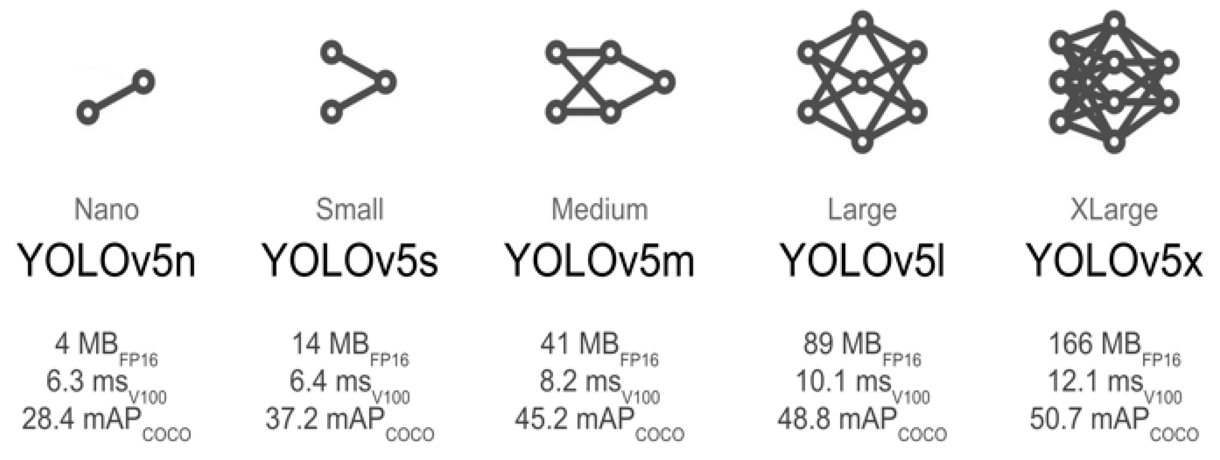
The initial model selected to be applied to the system is YOLOv5s (hereafter, defined as ‘basic’). Hyperparameters set up for model learning are shown in

Table 2. Model learning environment (hyperparameters).

Hyperparameters
Epoch	300
Batch size	16
Image size	640 × 640
Learning rate	0.01

. Epoch, Batch size, Image size, and Learning rate are set to 300, 16, 640 × 640, and 0.01. The hyperparameter value is not changed to identify the tendency of the technique used in this study, and model training is conducted by applying the basic value. Afterwards, performance analysis according to changes in hyperparameters is conducted for further model optimization. The model learning environment is presented in

Table 3. Model learning environment (hardware).

Hardware
Graphic	GeForce RTX 3090
CPU	i9-10900X
Memory	64 GB

.

The initial model of the system refers to a model without any technique applied. Its mAP and inference time are approximately 95.3 and 1.6 ms, respectively. We set the initial model as a performance comparison criterion for future performance-enhanced models. We aimed to improve the performance using three performance enhancement techniques (structure modification, model scaling, and lightweight design) to find the optimized model for the system. In Section 3, learning conditions and comparative analysis of results obtained by applying three techniques are presented. Conditions for each technique are set up directly, and the reason why there are various conditions is to analyze the tendency of the technique. The hyperparameters and hardware are equally used in the learning in each case.

4.1. Case Study

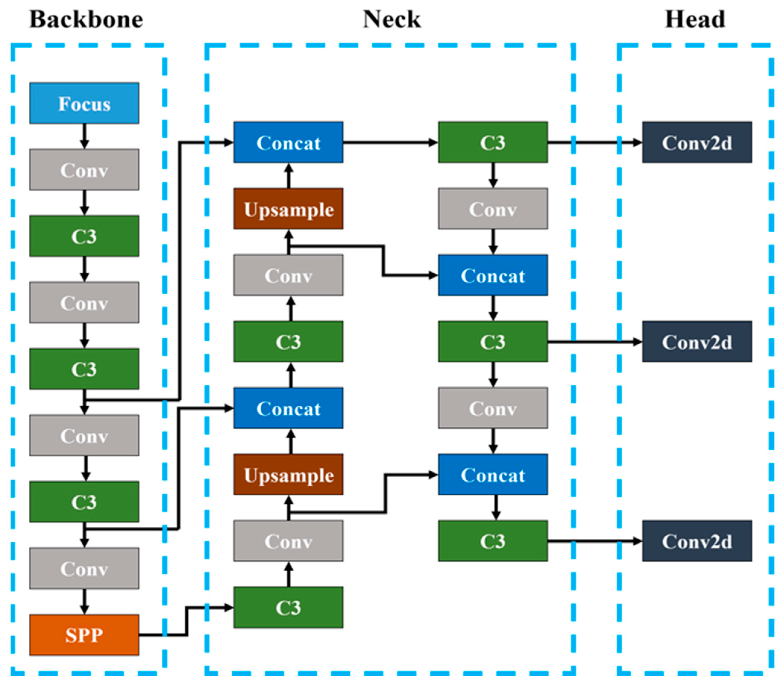
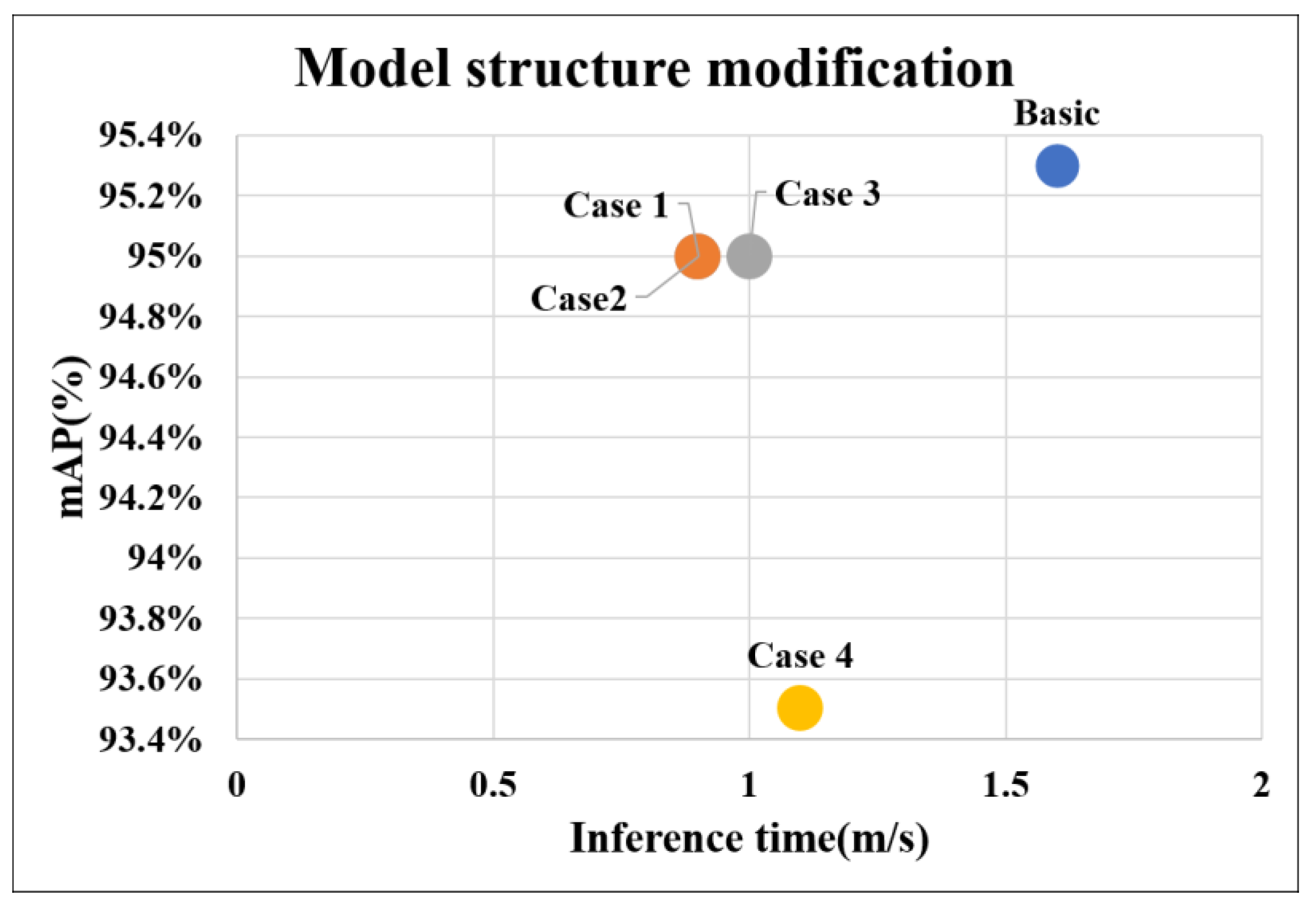
To improve the performance of the YOLOv5 model, we analyzed techniques on performance improvements as model and dataset modifications. A Conv block was added to the backbone in the YOLOv5s model. The model learning was conducted for four cases as shown in Figure S1 and performance results were comparatively analyzed.

As shown in Figure 14, the mAP and inference time of Cases 1 and 2 are approximately 95% and 0.9 ms, those of Case 3 were approximately 95% and 1.0 ms, and those of Case 4 were approximately 93.5% and 1.1 ms, respectively. In conclusion, Cases 1 and 2 had higher mAP and faster inference times than those of Cases 3 and 4 despite having fewer number of layers. This result verifies that the performance did not increase as the model’s depth increased, which is easily known in a deep learning model.

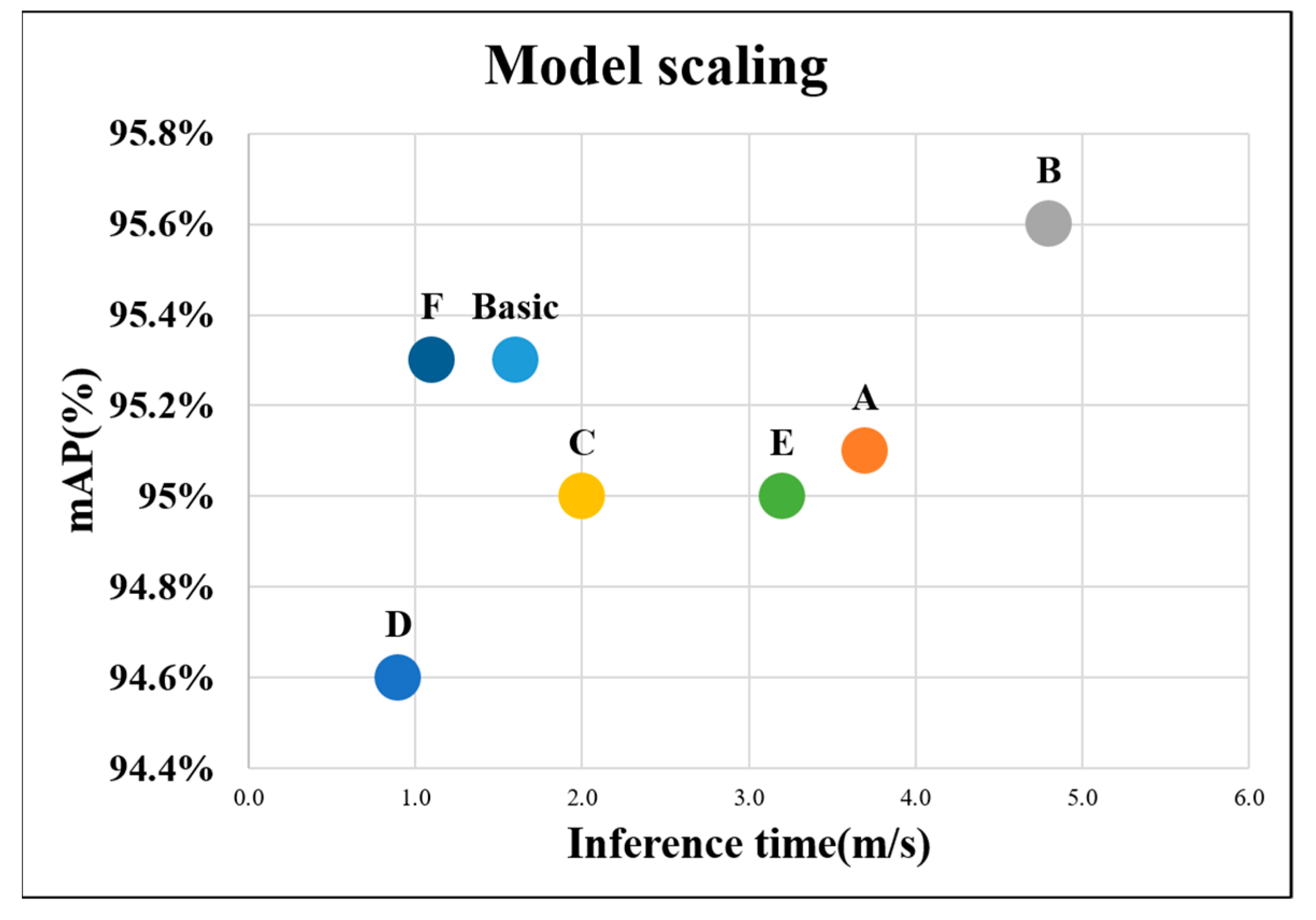
In model scaling, various values are applied to the models to find the optimized model for the proposed system. The model learning is conducted by applying seven cases of different model depths and widths, including the initial model of the system to compare the results.

Table 4. Model scaling.

	Depth	Width
Basic	0.33	0.50
A	0.33	1.00
B	0.67	1.00
C	0.67	0.50
D	0.67	0.25
E	0.33	0.75
F	1.00	0.25

summarizes the model scaling values of model depth and width, which are applied during model learning. Figure 15 shows the graph summarizing mAP and inference time.

When a ratio of 0.67 and 1.00 for the model depth and width, respectively, was applied, the highest mAP value of approximately 95.6% was obtained; further, when a ratio of 0.67 and 0.25 was applied, mAP was the lowest at approximately 94.6%. In 6 cases, except for the initial model, when a ratio of 1.00 and 0.25 for the model depth and width, respectively, was applied, mAP and inference time were approximately 95.3% and 1.1 ms, respectively, which is the most suitable model for the system.

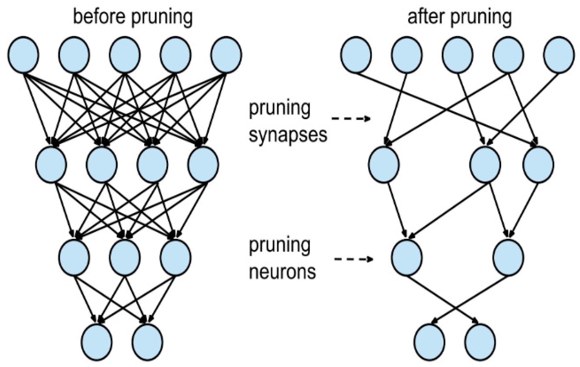
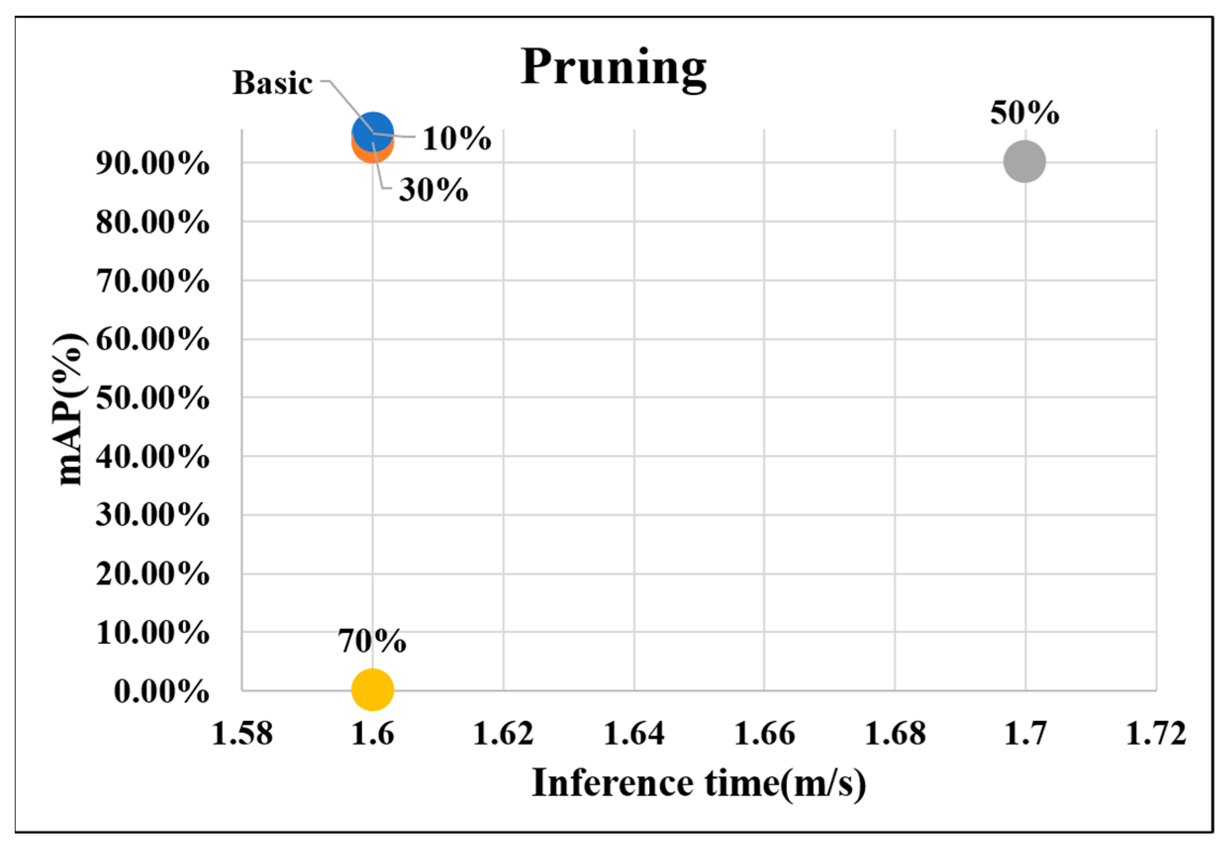
To analyze the trend of model performance that is revealed through the change in pruning value and find the suitable model, 4 cases of pruning values—10%, 30%, 50%, and 70%—were analyzed.

Figure 16 shows the graph summarizing the results of the four cases. When the pruning values were 10%, 30%, 50%, and 70%, mAP values were approximately 95%, 93.5%, 90.2%, and 0.0601%, and the inference times were 1.6, 1.6, 1.7, and 1.6 ms, respectively.

In conclusion, the performance tended to decrease as the lightweight value increased. Thus, the best performance was exhibited when the lightweight technique was set to 10%, which is the most suitable model for the system.

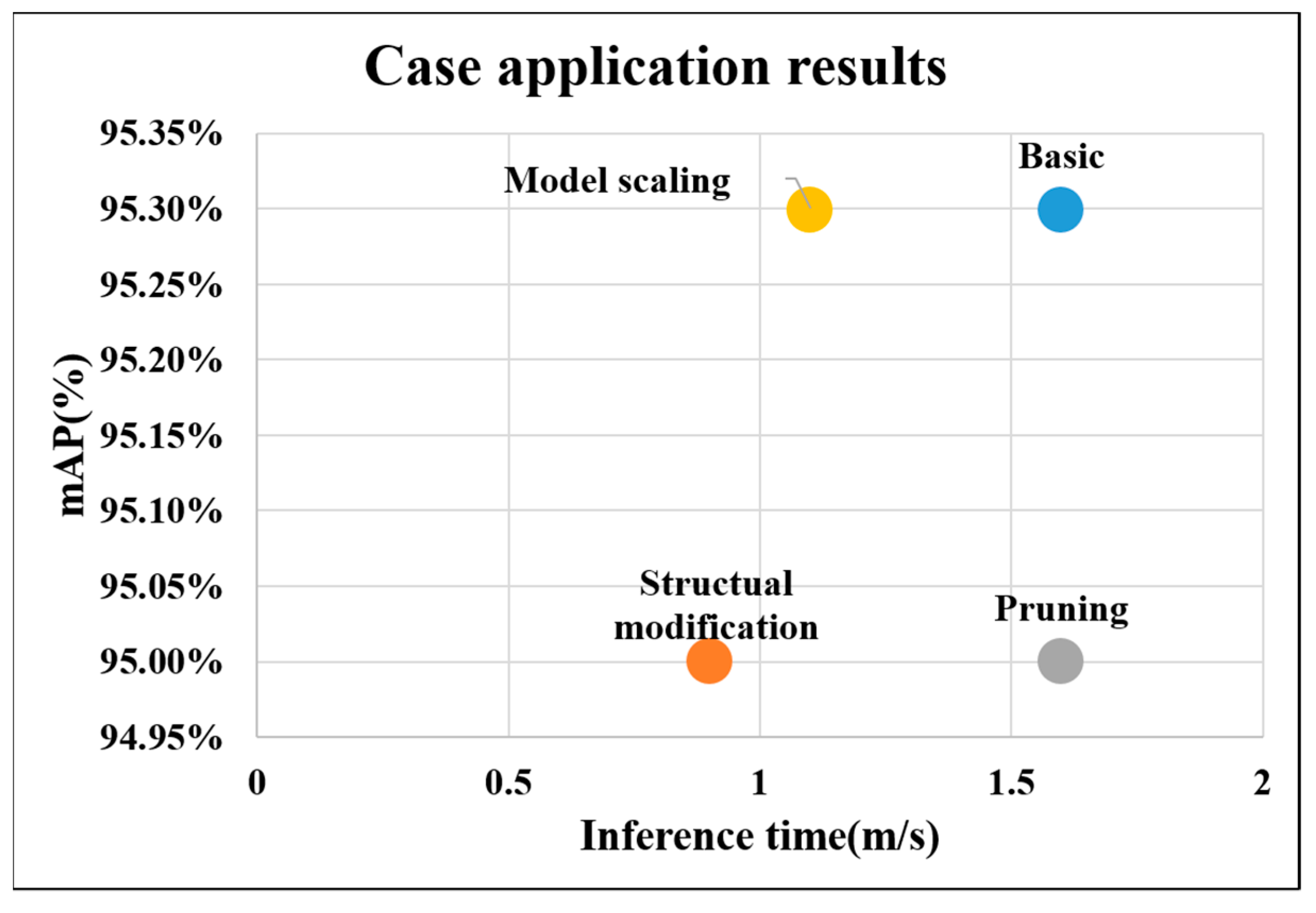
4.2. Analysis of Case Application Results

To find a suitable model for the defect detection system, three model improvement techniques were applied and their results were comparatively analyzed except for the initial model of the system.

In the case of structure modification, when one or two Conv blocks were added to the backbone, mAP was approximately 95% and the inference time was 0.9 ms, which was found to be the most suitable model for the system. In the case of model scaling, when a ratio of model depth and width (1.00 and 0.25) was applied, mAP was approximately 95.3% and the inference time was 1.1 ms, which was found to be the most suitable model. Finally, in the case of the lightweight technique, when 10% of the pruning value was applied, mAP was approximately 95% and the inference time was 1.6 ms, which was found to be the most suitable model for the system.

Figure 17 shows a graph comparing the most suitable models obtained using the three techniques applied to improve the performance of the initial system model. As verified in Figure 16, when the initial model and the case of applying the lightweight technique were compared, the same inference time was revealed; however, the mAP value was relatively lower in the case of pruning. In the case of model scaling, the same mAP was exhibited, but the inference time was faster. Finally, in the case of structure modification, mAP was lower than that of the initial model, but the inference time was the fastest. In this study, the model that applied model scaling was selected as the most suitable model for the proposed system because it has the same mAP value as that of the initial model but a faster inference time based on the criteria that false defect detection should be low in practical inspection although faster inference time is preferred for the system application.

AP values for each class were analyzed through

Table 5. mAP analysis (model scaling).

		Precision	Recall	AP
Basic	OK	0.802	0.896	0.904
	NG	0.975	0.822	0.929
	T-OK	0.855	0.966	0.983
	T-NG	1	0.985	0.995

. The AP values of ‘T-OK’ and ‘T-NG’ were high at about 98.3% and 99.5%, respectively. On the other hand, the AP values of ‘OK’ and ‘NG’ were measured relatively low at about 90.4% and 92.9%. Therefore, classes that measure relatively low AP values rather than the entire class should perform better.

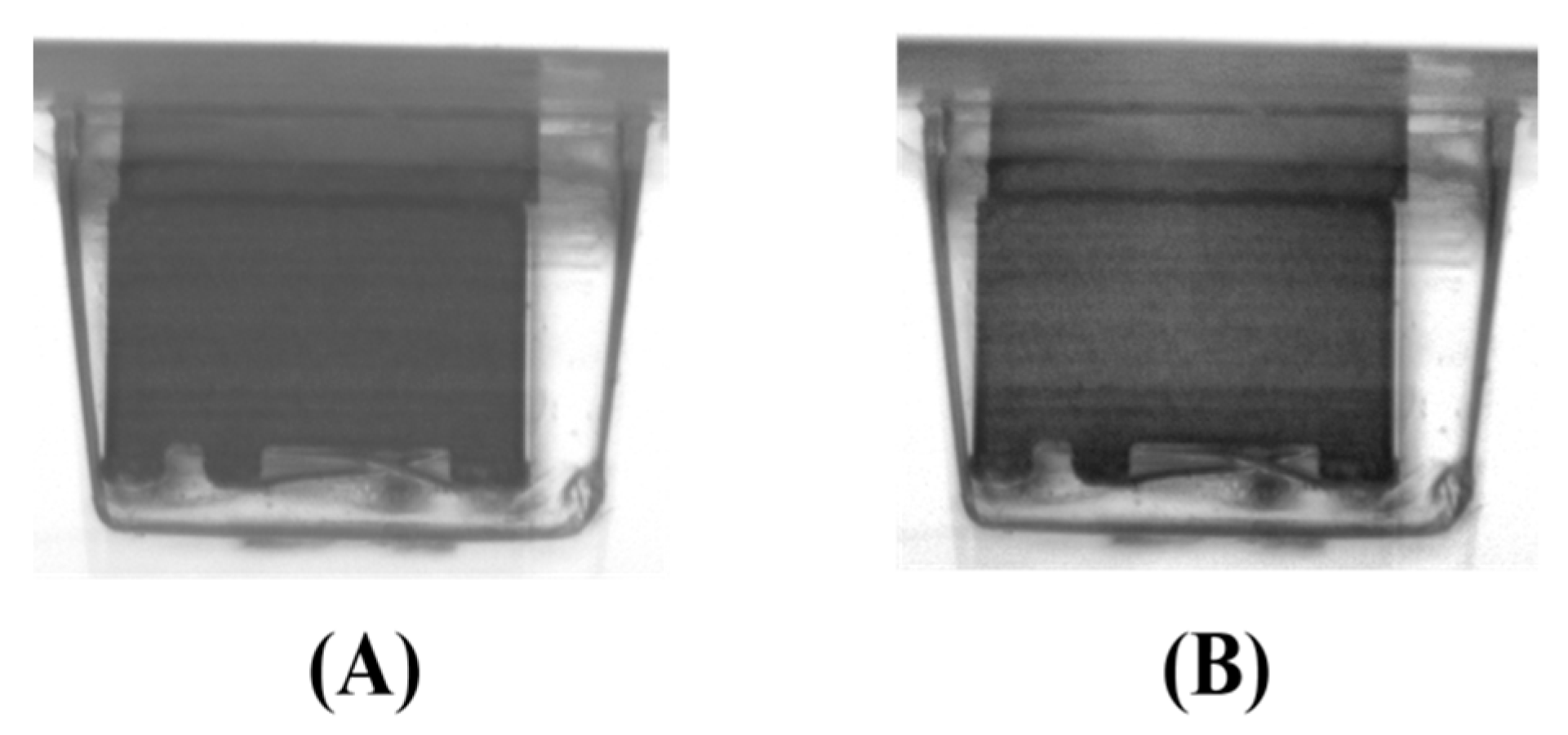
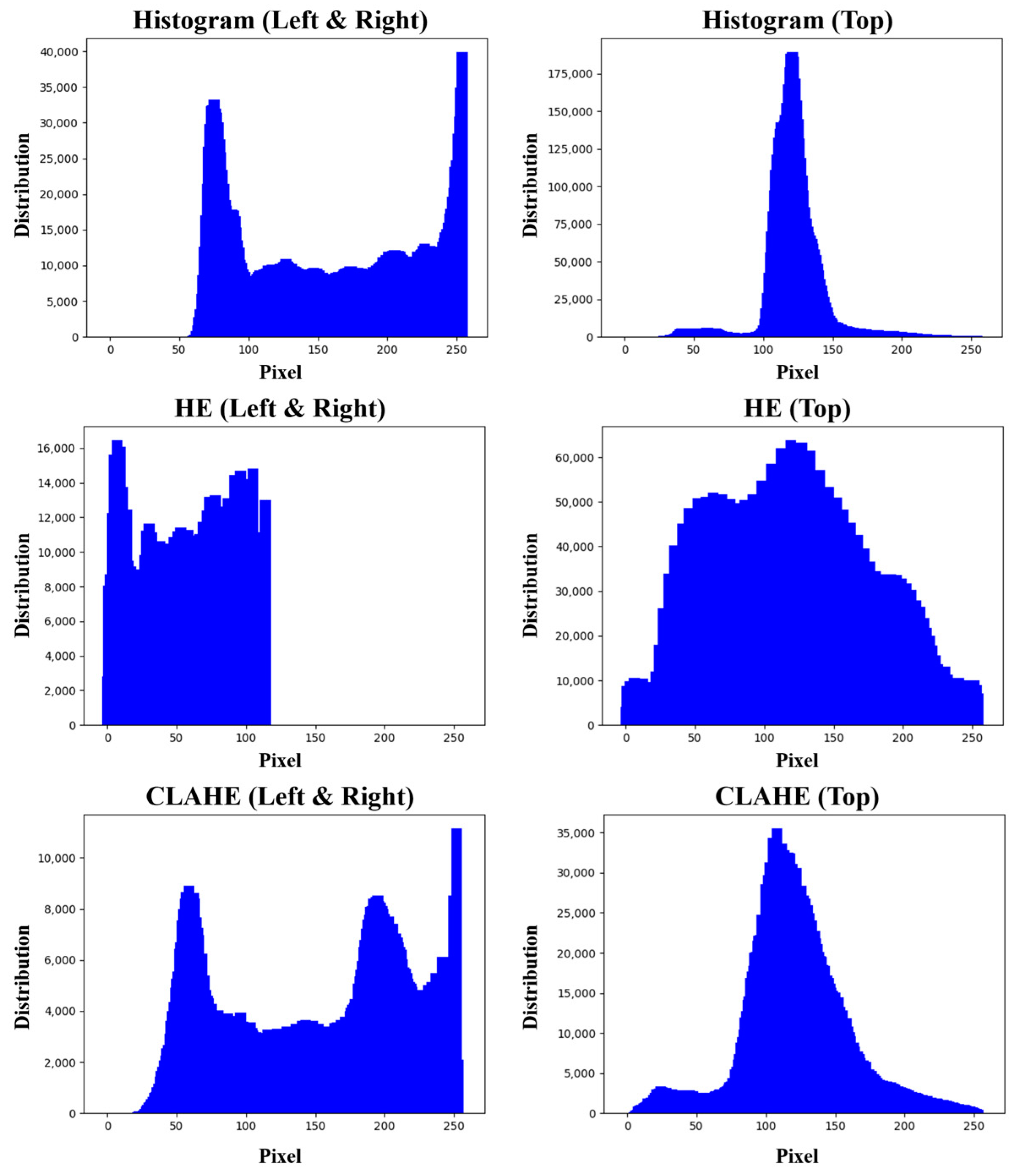
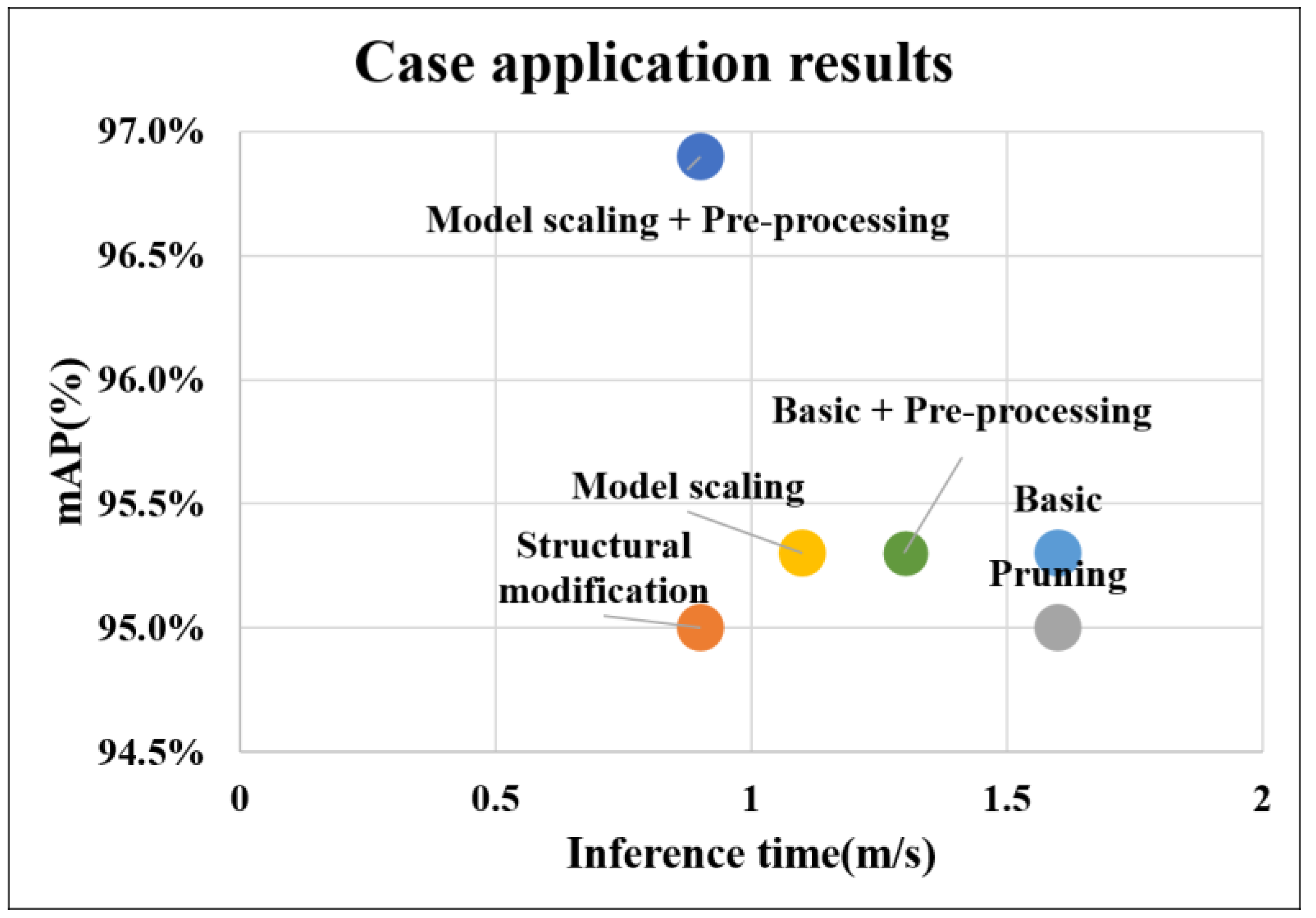
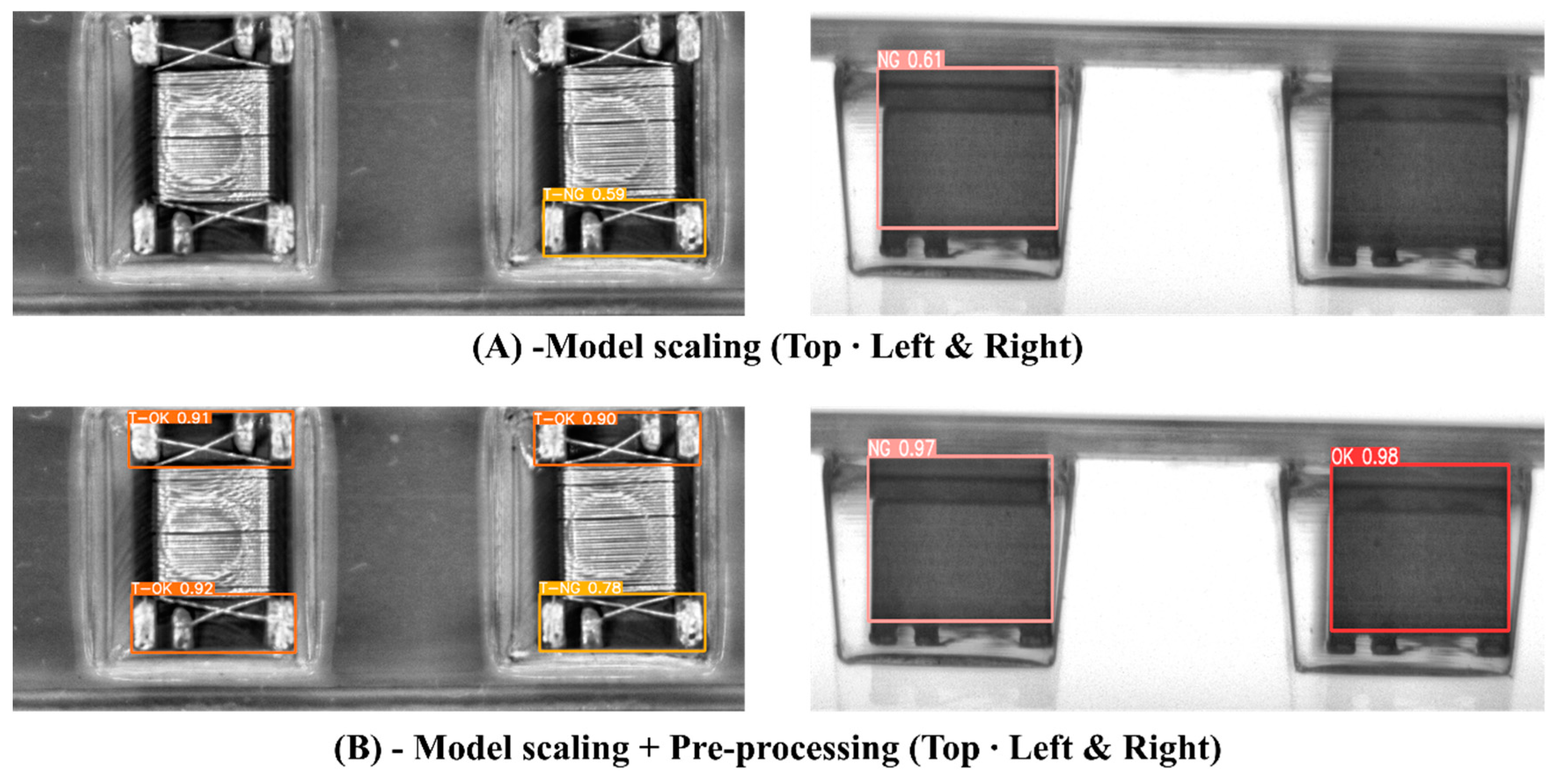
CLAHE was applied to the original dataset to further improve model performance, and model training was conducted in the same way as the model learning conditions of the model scaling, which was analyzed as the best model in Figure 18. We aimed to find suitable parameters of CLAHE using the SSIM image similarity measurement technique. SSIM was used to calculate the similarity of 1000 images of original data extracted randomly from “Top,” “Left,” and “Right” classes and CLAHE-applied data.

Table 6. SSIM results (grid size).

	8	16	32
Top	0.855699131	0.850566568	0.839055953
L and R	0.96406197	0.951937665	0.940069685

presents the calculation results obtained using 3 different grid sizes (8, 16, and 32), where the similarity is the highest when the grid size is 8 in all classes.

Based on the results in Table 6, CLAHE-applied data with a grid size of 8 were added to the original dataset to perform learning. The added dataset contained 7600 images. Thus, a total of 20,541 images were used in model learning. Figure 18 shows the results of training by adding data applying CLAHE to the basic model and the model applying model scaling, respectively. The final result shows that mAP were approximately 95.3% and 96.9% and the inference times were 1.3 ms and 0.9 ms. When analyzing the mAP value through

Table 7. mAP analysis (model scaling and pre-processing).

		Precision	Recall	AP
Our Model	OK	0.918	0.954	0.981
	NG	0.879	0.786	0.915
	T-OK	0.874	0.993	0.984
	T-NG	1	0.976	0.995

, it was observed that the mAP values of the ‘T-OK’ and ‘T-NG’ classes were maintained, and the mAP values of the ‘OK’ classes were improved. However, the value of ‘NG’ was relatively lowered by about 1.4%.

For further model optimization, performance analysis was conducted according to changes in hyperparameters.

Table 8. Performance resolution based on hyperparameters.

		Precision	Recall	mAP
Epoch	100	0.917	0.890	0.944
	150	0.915	0.897	0.951
	200	0.926	0.883	0.950
	400	0.907	0.901	0.948
Learning rate	0.001	0.924	0.897	0.953
	0.1	0.887	0.909	0.939

below summarizes the results of applying hyperparameter changes. The performance change according to the epoch shows the best performance when the epoch is 300. The learning rate shows the best performance in the cases of 0.01 and 0.001. Therefore, the optimal hyperparameter in this study is when the Epoch is 300 and the learning rate is 0.01 or 0.001. Based on this, it can be determined that the existing hyperparameters are appropriate for this study.

4.3. Result Analysis and Discussion

4.3.1. Results Analysis

Figure 18 shows that the model trained by adding CLAHE-applied data to model scaling applied model exhibits the best performance. However, it is a numerically very weak performance improvement result. Therefore, we tried to compare the results by extracting inference results using the model. Figure 19A shows the results extracted using the applied model scaling model that was found to be suitable in Figure 18. It verifies that only two classes (‘NG’ and ‘T-NG’) were extracted from four classes in the real results. Its mAP value was also approximately 61% for the ‘NG’ class and approximately 59% for the ‘T-NG’ class.

Meanwhile, Figure 19B verifies that all four classes were extracted. Except for the ‘T-NG’ class, all other classes showed more than 90% of mAP. Compared with the aforementioned results, the mAP of the ‘NG’ class increased by approximately 36% and that of the ‘T-NG’ class increased by approximately 19%.

Table 9. Analysis of mAP between YOLOv5 models.

	YOLOv5s (Basic)	YOLOv5m	YOLOv5l	YOLOv5s (CLAHE)	Our Model
mAP	95.3%	95.1%	95.6%	95.3%	96.9%

shows YOLOv5’s large and medium as analysis comparison targets for additional model analysis. The performance of the large and medium models of YOLOv5 was 95.6% and 95.1, respectively. This is an improved performance compared with the small model of YOLOv5, the basic model of this study, but it is lower than the performance of the proposed model, 96.9%. In addition, even when training was conducted by adding data applied with CLAHE from the basic model, the results were about 1.6% lower than the proposed model.

Table 10. Comparison of the number of inspections per second.

	Inspector	Basic Model	Our Model
Inspection of 1000 coils	Around 100–150 s	Around 63–83 s	Around 50–70 s

presents the comparison results of the number of inspections per second using human inspectors and the proposed model. Existing inspectors can inspect one side of the coil at a rate of around 10 coils per second. By contrast, the proposed model in this study takes approximately 0.9 ms to inspect one side of the coil, which gives a rate of around 1111 coils per second. However, this is a numerical result. When on-site tests were conducted with 1000 coils of data for the field applicability check, it took around 50–70 s. In summary, if this amount is inspected by a human inspector, it takes around 100–150 s, but the proposed YOLOv5 model takes nearly half the time.

4.3.2. Discussion

In comparison with structural modifications and lightweight approaches, model scaling proved to be the most effective technique for enhancing performance and achieving optimal results in model optimization. Additionally, data augmentation was employed to further boost performance. During this process, learning conditions were meticulously designed to identify the optimal model, and a detailed analysis of the results was conducted. Compared with other performance improvement techniques, applying model scaling, which varies the ratio of depth and width in the model, yields the best outcome. When analyzing the results of model scaling, increasing the depth and decreasing the width relative to the base model demonstrated the most favorable results.

Upon analyzing the final model, the proposed model in this study exhibited improved performance compared with the basic models of YOLOv5. However, a limitation of this work is the lower AP values for the ‘NG’ class when analyzing each class. Moreover, while the actual inspection time was faster than that of a human inspector, there was no substantial difference compared with the basic model of YOLOv5. To address this issue, various failure data can be additionally collected and utilized for model training to rectify the class-related problems. This will enhance the performance across all classes of the proposed model.

5. Conclusions and Future Research

In this study, a deep-learning-based coil quality inspection model was optimized. The study was conducted through three processes (‘Constructing a coil image data set using a prototype’, ‘YOLOv5 model optimization (to find the optimal parameter value) with 3 techniques: structure modification, model scaling, and lightweight’, ‘Data addition and model training with the CLAHE technique for dataset augmentation’). Through the above process, various results were analyzed. Finally, the model with model scaling and CLAHE showed the best performance, and the performance improvement of the coil defect detection model was up to approximately 1.6% compared with the base model. Although this study focused on small objects, it is expected to have future use in various fields such as manufacturing, machinery, and shipbuilding. Moreover, image preprocessing techniques were analyzed to additionally apply techniques suitable for research subjects and for use as new datasets. Finally, we would like to proceed with additional model optimization using algorithms other than those applied to YOLOv5.

References

1. Kim, J.T.; Jo, H.Y.; Choe, E.J. Recent Application Trends in Machine Vision Technology Using Deep Learning Techniques. Mag. IEIE 2016, 43, 18–26. [Google Scholar] [CrossRef]
2. Koh, D.M.; Choi, K.S. Accurate PCB Outline Extraction and Corner Detection for High Precision Machine Vision. J. Semicond. Disp. Technol. 2017, 16, 53–58. [Google Scholar]
3. Mohd, S.H.N.; Ab, R.M.Z.; Sulaiman, M.; Shukor, A.Z. Vision based Identification and Classification of Weld Defects in Welding Environments: A Review. Indian J. Sci. Technol. 2016, 9, 20. [Google Scholar]
4. Yao, J.; Qi, J.; Zhang, J.; Shao, H.; Yang, J.; Li, X. A Real-Time Detection Algorithm for Kiwifruit Defects Based on YOLOv5. Electronics 2021, 10, 1711. [Google Scholar] [CrossRef]
5. Zhu, L.; Zhang, J.; Jia, C. An Improved YOLOv5-based Method for Surface Defect Detection of Steel Plate. In Proceedings of the 2022 China Automation Congress (CAC), Xiamen, China, 25–27 November 2022. [Google Scholar]
6. INNOPOLIS. Machine Vision Market. 2021. Available online: https://www.innopolis.or.kr/board/view?linkId=46150&menuId=MENU00999 (accessed on 17 April 2023).
7. Zou, Z.; Chen, K.; Shi, Z.; Guo, Y.; Ye, J. Object detection in 20 years: A survey. arXiv 2019, arXiv:1905.05055. [Google Scholar] [CrossRef]
8. Alibek, E.; Kim, K.C. Metal Surface Defect Detection and Classification using EfficientNetV2 and YOLOv5. J. KIECS 2022, 17, 577–586. [Google Scholar]
9. Kim, I.S.; Lee, M.G.; Jeon, Y. Comparative Analysis of Defect Detection Using YOLO of Deep Learning. J. Korean Soc. Manuf. Technol. Eng. 2021, 30, 514–519. [Google Scholar]
10. Zhao, Z.; Yang, X.; Zhou, Y.; Sun, Q.; Ge, Z.; Liu, D. Real-time detection of particleboard surface defects based on improved YOLOV5 target detection. Sci. Rep. 2021, 11, 21777. [Google Scholar] [CrossRef] [PubMed]
11. Usamentiaga, R.; Lema, D.G.; Pedrayes, O.D.; Garcia, D.F. Automated Surface Defect Detection in Metals: A Comparative Review of Object Detection and Semantic Segmentation Using Deep Learning. IEEE Trans. Ind. Appl. 2022, 58, 4203–4213. [Google Scholar] [CrossRef]
12. Yun, J.P.; Shin, W.C.; Koo, G.; Kim, M.S.; Lee, C.; Lee, S.J. Automated defect inspection system for metal surfaces based on deep learning and data augmentation. J. Manuf. Syst. 2020, 55, 317–324. [Google Scholar] [CrossRef]
13. Feng, Z.; Guo, L.; Huang, D.; Li, R. Electrical Insulator Dfects Detection Method Based on YOLOv5. In Proceedings of the 10th Data Driven Control and Learning Systems Conference, Suzhou, China, 14–16 May 2021. [Google Scholar]
14. Wang, J.; Fu, P.; Gao, R.X. Machine vision intelligence for defect inspection based on deep learning. J. Manuf. Syst. 2019, 51, 52–60. [Google Scholar] [CrossRef]
15. Jocher, G.; Stoken, A.; Chaurasia, A.; Borovec, J.; NanoCode012; TaoXie; Kwon, Y.; Michael, K.; Liu, C.; Fang, J.; et al. Ultralytics/Yolov5: v6.0—YOLOv5n ‘Nano’ Models, Roboflow Integration, TensorFlow Export, OpenCV, DNN Support. 2021. Available online: https://github.com/ultralytics/yolov5 (accessed on 17 April 2023). [CrossRef]
16. Wang, C.Y.; Liao, H.Y.M.; Wu, Y.H.; Chen, P.Y.; Hsieh, J.W.; Yeh, I.H. CSPNet: A new backbone that can enhance learning capability of cnn. In Proceedings of the IEEE Conference on Computer Vision and Pattern Recognition Workshop, Seattle, WA, USA, 14–19 June 2020. [Google Scholar]
17. He, K.; Zhang, X.; Ren, S.; Sun, J. Spatial Pyramid Pooling in Deep Convolutional Networks for Visual Recognition. IEEE Trans. Pattern Anal. Mach. Intell. 2015, 37, 1904–1916. [Google Scholar] [CrossRef] [PubMed]
18. Liu, S.; Qi, L.; Qin, H.; Shi, J.; Jia, J. Path aggregation network for instance segmentation. In Proceedings of the IEEE Conference on Computer Vision and Pattern Recognition, Salt Lake City, UT, USA, 18–22 June 2018; pp. 8759–8768. [Google Scholar]
19. Lin, T.Y.; Dollar, P.; Girshick, R.; He, K.; Hariharan, B.; Belongie, S. Feature pyramid networks for object detection. In Proceedings of the IEEE Conferecne on Computer Vision and Pattern Recognition, Honolulu, HI, USA, 21–26 July 2017; pp. 2117–2125. [Google Scholar]
20. Redmon, J.; Farhadi, A. YOLOv3: An incremental improvement. arXiv 2018, arXiv:1804.02767. [Google Scholar]
21. Hinton, G.; Vinyals, O.; Dean, J. Distilling the Knowledge in a Neural Network. arXiv 2015, arXiv:1512.03385. [Google Scholar]
22. Wu, H.; Judd, P.; Zhang, X.; Isaev, M.; Micikevicius, P. Integer quantization for deep learning inference: Principles and empirical evaluation. arXiv 2020, arXiv:2004.09602. [Google Scholar]
23. Han, S.; Mao, H.; Dally, W.J. Deep compression: Compressing deep neural network with purning, trained quantization and Huffman coding. In Proceedings of the International Conference on Learning Representations (ICLR), San Juan, Puerto Rico, 2–4 May 2016. [Google Scholar]
24. Wang, Z.; Bovik, A.C.; Sheikh, H.R.; Simoncelli, E.P. Image Quality Assessment: From Error Visibility to Structural Similarity. IEEE Trans. Image Process. 2004, 13, 600–612. [Google Scholar] [CrossRef] [PubMed]
Figure 1. Example of coil—visual inspection.
Applsci 13 05200 g001
Figure 2. Forecast of the global machine vision market [6].
Applsci 13 05200 g002
Figure 3. Diagram of the coil defect detection system.
Applsci 13 05200 g003
Figure 4. Experimental equipment for data acquisition and quality inspection.
Applsci 13 05200 g004
Figure 5. YOLOv5 network structure.
Applsci 13 05200 g005
Figure 6. CSPNet structure.
Applsci 13 05200 g006
Figure 7. Categories of YOLOv5.
Applsci 13 05200 g007
Figure 8. Pruning.
Applsci 13 05200 g008
Figure 9. Example of coil datasets.
Applsci 13 05200 g009
Figure 10. Defective coil image data.
Applsci 13 05200 g010
Figure 11. Example of CLAHE Grid.
Applsci 13 05200 g011
Figure 12. CLAHE-applied example.
Applsci 13 05200 g012
Figure 13. Histograms (HE and CLAHE).
Applsci 13 05200 g013
Figure 14. Result graph (structure modification).
Applsci 13 05200 g014
Figure 15. Result graph (model scaling).
Applsci 13 05200 g015
Figure 16. Result graph (pruning).
Applsci 13 05200 g016
Figure 17. Result analysis graph.
Applsci 13 05200 g017
Figure 18. Final result analysis graph.
Applsci 13 05200 g018
Figure 19. Inference results.
Applsci 13 05200 g019