Article

Signals Intelligence System with Software-Defined Radio

Department of Electronics and Computers, Faculty of Electrical Engineering and Computer Science, Transilvania University of Brasov, B-dul Eroilor nr. 29, 500036 Brasov, Romania
*
Author to whom correspondence should be addressed.
Appl. Sci. 2023, 13(8), 5199; https://doi.org/10.3390/app13085199
Submission received: 8 March 2023 / Revised: 13 April 2023 / Accepted: 18 April 2023 / Published: 21 April 2023
(This article belongs to the Section Computing and Artificial Intelligence)

Abstract

:
In this paper, we present the implementation of a system that identifies the modulation of complex radio signals. This is realized using an artificial intelligence model developed, trained, and integrated with Microsoft Azure cloud. We consider that cloud-based platforms offer enough flexibility and processing power to use them instead of conventional computers for signal processing based on artificial intelligence. We tested the implementation using a software-defined radio platform developed in GNU Radio that generates and receives real modulated signals. This process ensures that the solution proposed is viable to be used in real signal processing systems. The results obtained show that for certain modulation types, the identification is performed with a high degree of success. The use of a cloud-based platform allows quick access to the system. The user is able to identify the signal modulation using only a laptop that has access to the internet.

1. Introduction

With the accelerated development of wired communications, but especially of wireless mobile communications, both terrestrial and satellite, the available frequency spectrum is increasingly reduced and disrupted. The transmission and reception of modulated signals must be performed quickly to keep up with all the demands and efficiently to make full use of the frequency spectrum that is available. An effective way to develop a mobile communication system from the point of view of development time and system testing, as well as from a financial point of view, is to use “Software Defined Radio” (SDR) [1,2,3]. This concept allows the use of powerful dedicated signal processing hardware for system simulation, implementation, and testing. SDR reconfiguration allows a wide range of applications to be developed on the same hardware, all controlled by software.
SDR equipment is very versatile and efficient, but it also requires competent software. The use of artificial intelligence allows the creation of complex and efficient applications that can process a very large number of signals without the need to implement various classical algorithms [4,5,6], which are difficult to understand, translate into software code, and will run much slower than an artificial neural network. The artificial neural networks, once trained with a sufficiently large and complete data set, will be able to recognize and process the received signals in a proper way.
This paper presents the definition and implementation of a SIGINT System (“Signals intelligence”) based on the advanced software-defined radio concept (with programmable digital modulation schemes and software-defined signal processing blocks) and artificial intelligence. These two elements presented above, SDR and artificial neural networks, are used in this paper to identify and classify modulated signals that are received and found in the database used for training. This helps a lot in systems working with multiple data modulations, eliminating the need to implement a complex and inefficient system for identifying the received signal.
In addition to the economic efficiency of the envisioned solution and the high level of novelty it comes up with, this paper also includes the combination of broadband “front-end” equipment and powerful neural networks. They create a system that integrates artificial intelligence and deep learning techniques with the SDR platform.
In order to identify what is the current status in the field of SDR, artificial intelligence, and SIGINT, several papers were analyzed. The analyzed papers were selected to be as close as possible to the system envisioned within this paper. From these papers, we extracted what are the strong points and what can be performed to improve the available solutions.
In [7,8], the reasons why SDR is the concept that can be perfectly used in the development of SIGINT systems are described. It helps the manufacturers to overcome the biggest problems encountered when using standard processing equipment. The degree of processing required for military radio equipment is much higher and more specialized than in previous years. The continued presence of a hostile environment is an optimization problem that is slowly becoming more and more difficult to master. Optimizing to a level close to 100% in the case of very complex RF (radio frequency) systems is almost impossible to achieve. Over time the designers of such systems have relied on simplified models that do not fully correspond to reality and fail to accurately capture real signals. Even though the individual components were increasingly optimized, the final system was limited. All these problems can be removed by using new SDR platforms combined with deep neural networks [9]. In paper [10], the SDR concept and convolutional neural networks are used together to develop a system that uses noise to modulate standard I/Q (in-phase/quadrature) samples to increase data transmission security.
Another example of a system that combines SDR and artificial intelligence is DARPA’s (Defense Advanced Research Projects Agency) Colosseum [11]. This system has immense processing power that is used in the Spectrum Collaboration Challenge. This system contains 128 USRP (Universal Software Radio Peripheral) Ettus X310 with integrated FPGAs (field-programmable gate arrays) and ATCA-3671 systems with multiple FPGAs and servers with very powerful graphics cards used for artificial intelligence.
O’Shea [12] uses artificial intelligence in RF signal processing. He analyses the performance of a “ResNet” type network used for signal detection that can have 24 different types of modulation. In the first phase, a database is created consisting of 24 classes of modulated signals that are acquired for SNR (signal-to-noise ratio) values between [−20 dB, 30 dB]. Most of this data is used to train the neural network, and a smaller part is used to validate it and calculate detection accuracy. The system used consists of a computer with several dedicated video cards used for defining, training, and validating the network. In addition, two USRP B210s are used for transmitting and receiving RF signals.
Mostly, intelligent neural networks are used for processing information in a 2D format (images). The RF signals have a different structure than 2D signals, and they require the definition of a different type of network than those used for image detection and processing [13] or speech signal processing [14]. In [15], an intelligent “CNN” (convolutional neural network) neural network is presented. It is modified to analyze and detect complex and temporal RF signals.
Systems using artificial intelligence are efficient enough to process a very large amount of data. They are able to provide much faster results than any other classical algorithm. However, they also have certain limitations, being vulnerable in the event of an attack. In paper [16], the vulnerabilities of the intelligent network used in the paper [11] are analyzed. They discovered that deep learning algorithms used for signal classification are very susceptible to attacks because less signal power is needed for the attacker in order to produce misclassification, as compared to traditional jamming.
The versatility shown by artificial neural networks is high, offering a great diversity of uses even within the same domain. Shi presented in [17] a system that is capable of detecting and classifying: new signals received but known, new signals received but unknown, repeated attack signals received from a jamming station, and overlapping signals. Signal reception and processing were carried out for signals at SNR levels between [0 dB, 18 dB].
This paper comes up with a new type of approach that can be used for signal modulation detection. The goal of this paper is to assess the feasibility of performing cloud-based modulation recognition using artificial neural networks and SDR. The proposed approach uses cloud computing instead of traditional hardware (CPU (central processing unit) or GPU (graphics processing unit)) in order to obtain the trained model of the artificial intelligence network. The use of cloud computing removes the limits imposed by dedicated hardware equipment by providing sufficient processing power required by the neural network. The system integration is also performed in the cloud and allows the users to connect from everywhere. The only resources they need to use the system are a computer with internet access. Section 2 presents the experimental setup together with the system architecture and definition. Section 3 illustrates the results obtained after the network training and how the resulting model is tested against real data. The discussion of the results is presented in Section 4, while Section 5 presents the conclusions drawn.

2. Materials and Methods

2.1. Experimental Setup

The hardware used is BladeRF 2.0 micro xA4 [18]. This is a new generation SDR equipment. It has a low price, and it is dedicated to students and people who are passionate about SDR but who have a limited budget. The equipment is versatile because it can be used by most computer operating systems (Windows, Linux, and macOS). Two of these boards are used within the paper. The characteristics of the used boards are shown in Table 1. Applications and frameworks that support this board are GNU Radio, MATLAB, Simulink, and PothosWare. This device is also used in multiple research projects such as [19,20].
For the artificial neural network implementation, several solutions were analyzed. The analyzed solutions were selected in order to allow the implementation without being an expert in this field. The first two analyzed platforms were DLHUB [21] and ANNHUB [22]. Both of them are developed by the same company, ANSCenter (Sydney, Australia) [23]. The two platforms offer the user the opportunity to create training models in a simple and efficient way without the need for advanced knowledge in the field of artificial intelligence. The resulting model can be exported to multiple programming languages (LabVIEW, C++, Arduino, Python), where it can be integrated to form an entire system. Following the integrations and tests performed with these two platforms, the following disadvantages were found:
  • They require a computer with a very powerful processor and a dedicated video card to be able to successfully train the model;
  • The configurations available are implemented to obtain models of neural networks dedicated to image and video processing;
  • The training process of a model cannot run successfully if the number of input data is larger than 2048.
All these disadvantages determined after testing the platforms led to their non-use in this paper.
Another solution that can be used to develop and implement an artificial neural network consists of using cloud computing platforms. After analyzing the available platforms (Google Vertex AI (artificial intelligence), Microsoft Azure Auto ML (machine learning), Amazon AWS ML, IBM Watson Studio, and Oracle AI), only one was selected for further activities. The platform selected is Microsoft Azure AutoML [24]. This selection was made based on the ratios between price and performance and between configurability and performance. AutoML is a service developed by Microsoft within its research division. Its main purpose is to speed up the time needed to develop a neural network and obtain dedicated models as simply and quickly as possible. This is a big advantage over the classical approach, where powerful hardware equipment, multiple knowledge in the field of artificial intelligence, and a lot of time for analysis and development are needed. Azure AutoML enables researchers and developers to create artificial intelligence models that can be used to solve various problems, save a lot of time that would be required to develop a classic application, and streamline various processes. The three main types of processing possible within AutoML are classification, regression, and prediction [25]. The processing type used within this paper is classification. Classification is one of the most common types of AI applications. Using the data provided for training, the resulting model can predict which category new data entered into the model falls into.
The SDR framework used to develop the applications that send and receive data used for testing is GNU Radio. GNU Radio is a dedicated framework for SDR applications. It is used to create topologies consisting of the interconnection of several dedicated blocks for digital signal processing. These topologies can be created and tested both graphically and textually using the Python programming language. Once created, a topology can be run both locally and across the network. GNU Radio also offers the possibility of making dedicated blocks for signal processing. If the resources required by the processing blocks are high, they can be moved and integrated to run in Soc (FPGA) or DMA (direct memory access) devices. In addition to the ease with which the application can be used, there is also very good connectivity with the most used SDR hardware, such as USRP, HackRF, or BladeRF. For these and more, there are dedicated drivers that are compatible with GNU Radio and allow use with great ease. This framework can be installed on Windows, Ubuntu, Fedora, and macOS operating systems. The programming languages that can be used for development are “C/C++” and “python” [26].

2.2. System Architecture

The implemented system has an architecture based on the symbiosis between the two components: hardware and software. They intertwine to create a homogeneous and efficient system. Figure 1 shows how the system components are interconnected.
How the components of the system work and communicate can be seen in Figure 2. In the upper part of Figure 2, the components that are used to train and validate the artificial intelligence network are presented. The database, after it is prepared, is loaded in the Microsoft Azure Auto ML Service, where the artificial intelligence network is configured. Following the training and validation part, the trained model is realized. In the lower part of the image, the components used to test the trained model are presented. The SDR platform is used to send and receive modulated signals. The modulated samples received are inserted into the integrated trained model (integrated into Microsoft Azure cloud) that generates the answer with the identified modulation type.

2.3. System Definition and Testing

2.3.1. Database Preparation

The main step to obtaining an artificial intelligence model is to have a sufficiently large and complete database to allow training, validation, and testing of a model as efficiently as possible. To obtain the most valid results, the RF signal database called “RADIOML 2018.01A” [27], which was created and used for the first time in paper [12], was chosen as a starting point.
In this database, we find signals that are modulated using the following 24 modulation schemes: OOK, 4ASK, 8ASK, BPSK, QPSK, 8PSK, 16PSK, 32PSK, 16APSK, 32APSK, 64APSK, 128APSK, 16QAM, 32QAM, 64QAM, 128QAM, 256QAM, AM-SSB-WC, AM-SSB-SC, AM-DSB-WC, AM-DSB-SC, FM, GMSK, and OQPSK.
All these data are saved in the “hdf5” file format used especially for keeping multidimensional data strings. The data are split into three strings, each of which is used to describe a specific detail about the database. After analyzing the file, the following details about the three strings were extracted:
The first string has 2,555,904 recordings, each having 1024 complex elements. These elements represent the modulated signal samples.
The second string has the same number of elements in which the type of modulation the signal has is noted.
The third string has the same size as the previous two, these containing a single element, each having values starting with −20 and ending with 30 signifying the SNR level in dB at which the signal was acquired.
To obtain the desired dataset for training the artificial network, only records for the following ten modulation classes were extracted from the database: OOK, 4ASK, 8ASK, BPSK, QPSK, 8PSK, 16PSK, 32PSK, FM, and GMSK. Additionally, these are the investigations and research scenarios used in our paper. Only these ten modulations were selected because they are enough to validate our approach, and many of them are used in mobile communications.
For each of these 10 classes, 1024 training records and 256 testing records were extracted for each of the SNR levels between [2 dB, 30 dB]. A total of 153,600 records are available for training and 38,400 for testing, with each of them having 1024 complex elements.
It was decided to use a smaller number of modulation classes at higher SNR levels to obtain a model that performs better at high SNR. However, if the SNR is low, the detection rate of any intelligent network is very low because the modulation pattern is not easily detected; this can be seen in [12,15].
In order to extract the samples from the dataset, a shell script was used. The script has put the data in a separate folder for each modulation and inside the modulation folder in separate folders for test and training. The extracted complex data is written to a “CSV” (comma-separated values) file, which is the final database that is used for training, validation, and testing. In Table 2, the internal structure and content of the database can be seen.
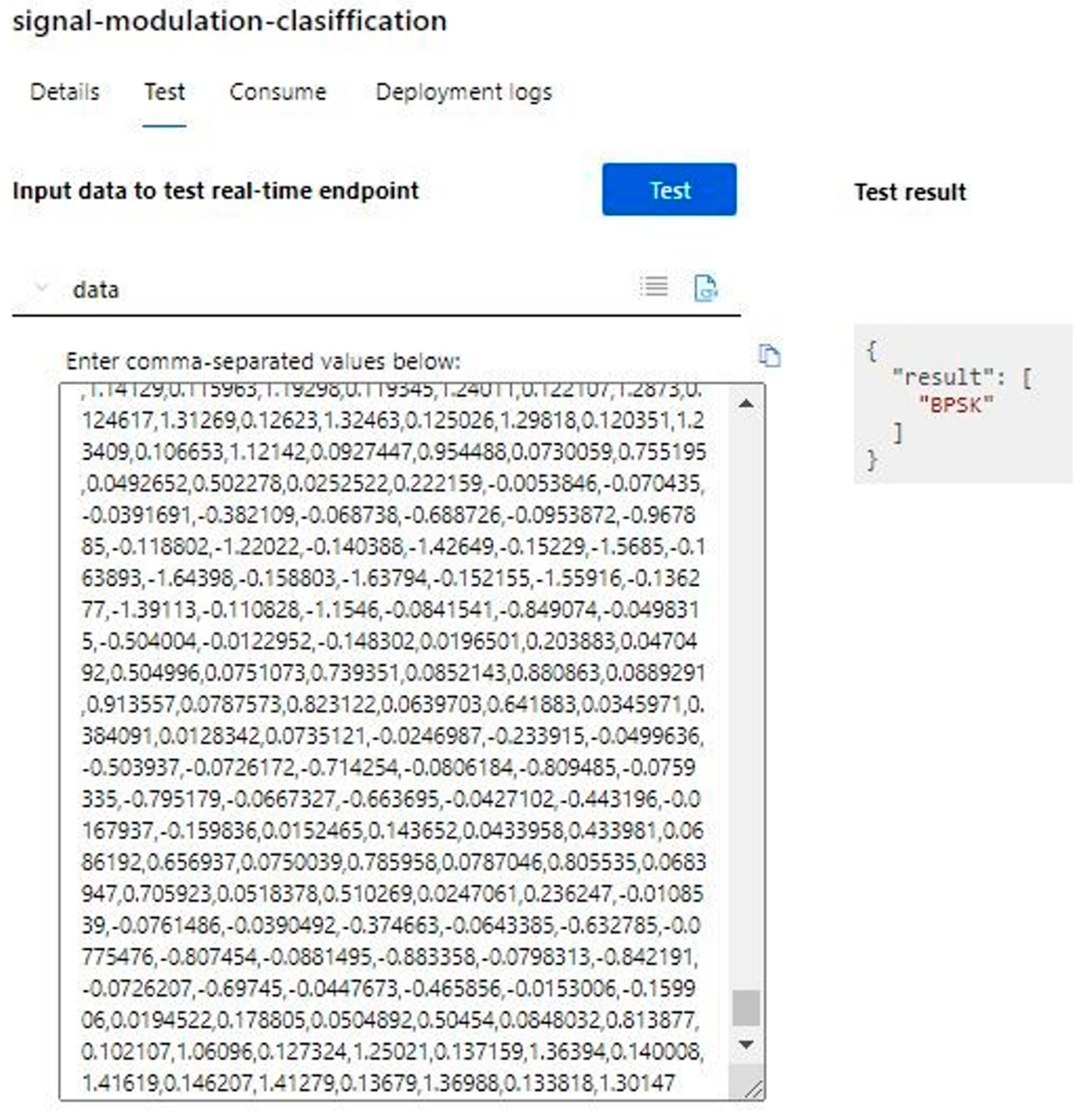
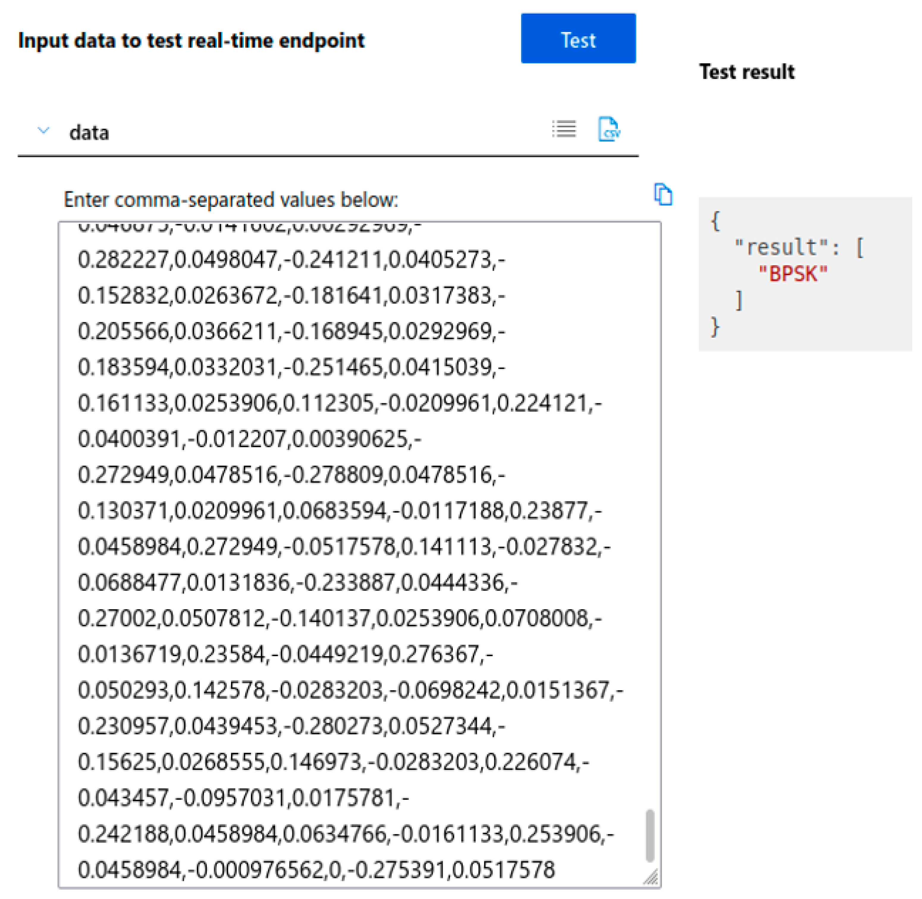
The extracted data is written in a “CSV” file to ensure compatibility with the “Azure AutoML” service that is used to train and integrate the intelligent network. It must be clearly defined which data constitutes the inputs from which the characteristics necessary for training will be extracted and which data represent the outputs according to which the classification of the obtained results will be carried out.
Each signal describing a modulation type consists of 1024 complex values. These complex values are divided into the real part and the imaginary part of the complex number. These are then arranged in rows describing each of the 1024 real values and 1024 complex values. Each column has a header describing the index of each value. At the end, a final column is inserted where the type of signal characterized by the input values is described.
The headers are very important because they are used to train and then validate and test the AI model.

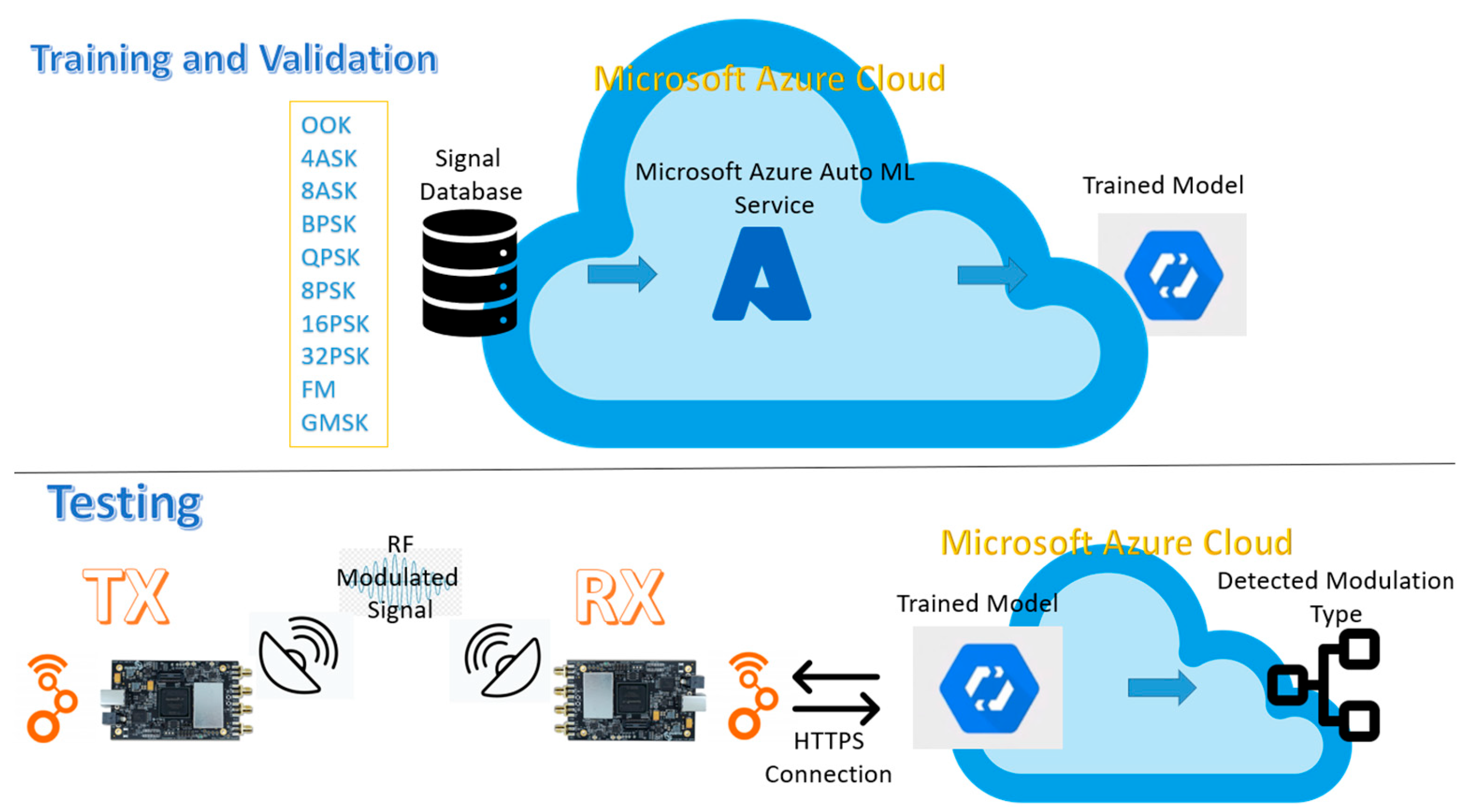
2.3.2. Network Training

Automated ML functionality from the “Microsoft Azure AutoML” service was used to define, train, test, and validate the intelligent network. After the definition of the new model has been started, the database that is used for training and validation is chosen. The next step is to analyze the data to identify potential problems. As possible problems, the following can be mentioned: missing data in certain columns, not all input data having the same format, or for some input data, we do not have output data.
The training is configured to be performed using “Signal Type” as the target column. This column describes the type of signal that is characterized by the input data. As hardware support, a virtual machine is used with a 6-core CPU, 28 GB RAM (random-access memory), and 56 GB (gigabyte) storage memory.
To configure the model training, three options are available. From the three options, the model that performs data classification based on the input data is chosen. The “Deep Learning” option is also enabled to ensure a better extraction of the model’s features and to obtain a more efficient trained model. The first additional setting configured is the metric used. Accuracy is chosen because it best characterizes the model to be implemented. By accuracy, what is meant is the number of correctly predicted input data out of the total amount of data. It is chosen to use all possible algorithms to see exactly which one is the most efficient. The running time is set to the maximum possible of 24 h, which is the maximum training time offered for a model where the “Deep Learning” option is activated. No step is set for the validation metric, trying to obtain a result as close to perfection as possible. After all configuration work is complete, the training process is started.
The training process begins by checking several elements. The first thing that is checked is whether the input data is divided in an approximately equal way for each signal type. The second checked element is the lack of samples in any of the input vectors. The last element checked is if one or multiple samples from the input vectors have a value too high that may bias the detection result in a wrong way. By a much too high value is understood the fact that this value has an order of magnitude two or more times higher than the other samples from the rest of the data vectors. This value can spoil the detection because the model resulting from training with this data will always expect certain samples from the input data to have such high values, which will not happen if the data are correct.

3. Results

After completing the training process, a number of 46 models resulted, each of which has a certain accuracy value. Table 3 lists the first 16 models that achieved the best accuracy among the 46 generated.
For integration, the model with the highest accuracy is chosen. For this model, the results obtained from the validation of the model after its training are also generated.
The time required to obtain this model is 9 h, 21 min, and 19 s. During this time, both the actual training and the validation of the results were carried out. All the metrics obtained from the validation of this model are:
  • Accuracy = 0.64831;
  • Average macro precision = 0.68130;
  • Average micro accuracy = 0.79536.
The most important characteristic of the trained model is the confusion matrix. It can be seen in Table 4. As can be seen in the confusion matrix, the best results are recorded for the modulations: FM, BPSK, GMSK, OOK, and 4ASK. The worst results are recorded for the modulations: 8PSK, 16APSK, 32APSK, QPSK, and 8ASK.
The resulting accuracy differs for each modulation. Some modulations have a better accuracy than others. The accuracy for each modulation is listed in Table 5.

System Testing

To use the resulting artificial intelligence model, it needs to be integrated. Its integration is also carried out with the help of the “Microsoft Azure AutoML” service. To integrate the model, all the integration parameters need to be configured. This can take from a few minutes to a few hours, depending on the processing unit chosen. The “Azure Container Instance” service [28] was chosen as the processing unit because it allows quick integration, and the user does not have to manage virtual machines or other additional tools. This service allows the integration of the model without the need for additional elements.
After completing the integration process, we moved to the testing step to validate the obtained model. For the initial system testing, data sequences from the database are used. Multiple signals for each of the 10 modulation classes are stored in this database.
Signals for each of the 10 modulation classes are tested. The results obtained are in accordance with the obtained accuracy and the values in the confusion matrix. For signals that are collected at a lower SNR level, false detection is possible. The higher the signal strength level, the higher the possibility that the detection will be 100% correct.
The results of running the integrated model for a “BPSK” modulated signal can be seen in Figure 3. On the left side of the picture can be seen the text entry where the samples of the signal to be tested are pasted. After the “test” button is pressed, the identified modulation type is printed on the right side of the window. The result is available in a gray box in JSON (JavaScript Object Notation) format.
In order to test the obtained model in real conditions, an SDR test platform was used. In this, the transmission and reception of the modulated signal over a radio channel are carried out.
To implement the SDR part of the system, the following are used:
  • Two BladeRF 2.0 micro xA4 equipment as RF hardware equipment with additional accessories (antennas, SMA (SubMiniature version A) cables, USB (Universal Serial Bus) cables).
  • A laptop with the Ubuntu 18.04 operating system for running software applications and for interfacing with hardware equipment and the AI model.
  • GNU Radio topologies for realizing signal processing applications.
The first implemented topology can be seen in Figure 4. In this topology, “BPSK” transmission and reception are implemented. The data source is a random one that generates 8-bit integers with values between 0 and 255. The integers are divided into 1-bit symbols and “BPSK” modulated. The modulated symbols are then interpolated to achieve a rate of eight samples per symbol. After sampling, an RRC (root-raised-cosine) filter is applied to prepare the transmission samples. The transmission is carried out with a sampling frequency equal to 1 MHZ. The RF frequency on which the data are transmitted is equal to 2.45 GHz. The transmitted signal can be seen in Figure 5. The reception of the signal is performed on the same RF frequency as the transmission and with the same sampling frequency. The received samples are written in a “CSV” file. This file is then used in order to test the trained model.
The first check is performed for the samples corresponding to the signal with “BPSK” modulation. Samples are copied from the file resulting from transmission and reception and entered in the input data section of the integrated model. Once the data are entered, the user needs to press the “Test” button. To perform the detection, the model needs a few seconds. Once the detection process is completed, the result with the detected modulation appears on the right side of the screen. The result can be seen in Figure 6.

4. Discussion

In this paper, we have shown that signal processing can be performed using cloud computing. It can be used for artificial intelligence network definition, training, and deployment. This method enhances the traditional method of AI development for signal processing. Additionally, compared to the traditional way of using dedicated hardware, this method ensures similar results but in a faster and cheaper way.
We have shown that by having a good database with training samples and minimal knowledge of signal processing and neural networks, neural network models can be trained and deployed.
Compared to the standard approach of using neural networks on a local computer, cloud-based neural networks have both advantages and disadvantages. These are presented in Table 6, and they were extracted by comparing the results obtained in this paper with the ones obtained in paper [12].
In Table 7, a comparison between the results obtained in this paper and the results obtained in [12] using conventional neural networks is listed. This table shows that for BPSK, FM, OOK, and GMSK, the detection rate is similar. For the rest of the modulations, the difference is higher in favor of the conventional neural network developed on a local computer.
The main further research direction consists of improving the neural network model by using a database with more modulation types that have a wider range of noise and interference. Another future research direction consists of the integration of the trained model into a system that will detect modulation type in real-time and will be able to demodulate it directly without human intervention.

5. Conclusions

This new type of approach that uses cloud computing instead of traditional hardware (CPU or GPU) for artificial intelligence network training eliminates the limitations imposed by dedicated hardware devices. Having the system integrated into the cloud allows quick connection from all around. The user needs only a good internet connection to access and use the system.
This way of developing and integrating neural networks looks very promising and opens the door to all those who what to study the field of AI and signal processing. Although there are still many things to learn, we have shown that this is possible, and it can be achieved by working hard and dedicating enough time.
The system presented in this paper was envisioned, developed, and tested over the course of a year. The state-of-the-art phase lasted around three months. The artificial network model implementation and training were the most challenging. It took around six months to design and produce a model that fulfilled all the needs. The hardest part was choosing the cloud platform used and the artificial intelligence network model that would meet the system’s specifications. The system integration and testing were the last parts of the paper and lasted around three months.
To improve the current implementation, the authors intend to extend the modulation database with more data for each modulation in order to have a larger amount of data used to train the model. Additionally, more modulations will be added in order to obtain a model that can be used for a wider range of applications. To achieve the best possible model, multiple configurations of hardware and training parameters will be used. It was noticed that the accuracy decreases with the SNR. To overcome this problem, two possible methods will be used. The first one will consist of the implementation of extra processing steps used to improve the signal samples before they are given as input to the neural network. The second method will consist of another neural network model that will aim to reduce noise and improve signal quality. The selection between these two methods will be made after further analysis of both is performed.

Author Contributions

Conceptualization, F.R., T.C.B. and V.P.; methodology, F.R. and M.A.; software, F.R. and T.C.B.; validation, T.C.B. and V.P.; formal analysis, P.A.C. and D.T.C.; writing—original draft preparation, F.R.; writing—review and editing, M.A. and P.A.C.; visualization, D.T.C.; supervision, T.C.B. All authors have read and agreed to the published version of the manuscript.

Funding

This research received no external funding.

Data Availability Statement

Not applicable.

Conflicts of Interest

The authors declare no conflict of interest.

References

  1. Garg, V.K. (Ed.) Fourth Generation Systems and New Wireless Technologies. In The Morgan Kaufmann Series in Networking, Wireless Communications & Networking, Morgan Kaufmann; Elsevier: Amsterdam, The Netherlands, 2007; pp. 1–22. ISBN 9780123735805. [Google Scholar] [CrossRef]
  2. Javier, A.; Marian, U.; Dongho, Y. Integrating software-defined radios. In Computing in Communication Networks; Frank, H.P.F., Fabrizio, G., Patrick, S., Eds.; Academic Press: Cambridge, MA, USA, 2020; pp. 413–427. ISBN 9780128204887. [Google Scholar] [CrossRef]
  3. Tato, A. Software Defined Radio: A Brief Introduction. Proceedings 2018, 2, 1196. [Google Scholar] [CrossRef]
  4. Zhang, R.; Li, J.; Wu, J. A universal algorithm of modulation and demodulation. J. Electron. 2002, 19, 289–295. [Google Scholar] [CrossRef]
  5. Wang, C.; Qu, Y.; Tang, Y.P.T. IQ quadrature demodulation algorithm used in heterodyne detection. Infrared Phys. Technol. 2015, 72, 191–194. [Google Scholar] [CrossRef]
  6. Merz, R.; Botteron, C.; Farine, P.A. A novel low complexity data demodulation algorithm for pulse position modulation. Digit. Signal Process. 2012, 22, 535–543. [Google Scholar] [CrossRef]
  7. AI in Software Defined Radio. Available online: https://www.ni.com/ro-ro/innovations/white-papers/19/artificial-intelligence-in-software-defined-sigint-systems.html#section-1134962763 (accessed on 16 December 2022).
  8. Bonati, L.; Polese, M.; D’Oro, S.; Basagni, S.; Melodia, T. OpenRAN Gym: AI/ML development, data collection, and testing for O-RAN on PAWR platforms. Comput. Netw. 2023, 220, 109502. [Google Scholar] [CrossRef]
  9. Shevitski, B.; Watkins, Y.; Man, N.; Girard, M. Digital Signal Processing Using Deep Neural Networks. arXiv 2021, arXiv:2109.10404. [Google Scholar]
  10. Choi, J.; Dongryul, P.; Suil, K.; Seungyoung, A. Implementation of a Noise-Shaped Signaling System through Software-Defined Radio. Appl. Sci. 2022, 12, 641. [Google Scholar] [CrossRef]
  11. DARPA Colosseum. Available online: https://www.mwrf.com/technologies/test-measurement/article/21848345/darpas-colosseum-emulates-em-environments (accessed on 16 December 2022).
  12. O’Shea, T.J.; Roy, T.; Clancy, T.C. Over-the-air deep learning based radio signal classification. IEEE J. Sel. Top. Signal Process. 2018, 12, 168–179. [Google Scholar] [CrossRef]
  13. Krizhevsky, A.; Sutskever, I.; Hinton, G.E. Imagenet classification with deep convolutional neural networks. In Proceedings of the Advances in Neural Information Processing Systems, Lake Tahoe, NV, USA, 3–6 December 2012; pp. 1097–1105. [Google Scholar]
  14. Sainath, T.; Weiss, R.J.; Wilson, K.; Senior, A.W.; Vinyals, O. Learning the speech front-end with raw waveform cldnns. In Proceedings of the 16th Annual Conference of the International Speech Communication Association (INTERSPEECH 2015), Dresden, Germany, 6–10 September 2015. [Google Scholar]
  15. O’Shea, T.J.; Corgan, J.; Clancy, T.C. Convolutional radio modulation recognition networks. In Proceedings of the Engineering Applications of Neural Networks, Aberdeen, UK, 2–5 September 2016; pp. 213–226. [Google Scholar]
  16. Sadeghi, M.; Larsson, E.G. Adversarial attacks on deep-learning based radio signal classification. IEEE Wirel. Commun. Lett. 2018, 8, 213–216. [Google Scholar] [CrossRef]
  17. Shi, Y.; Davaslioglu, K.; Sagduyu, Y.E.; Headley, W.C.; Fowler, M.; Green, G. Deep learning for RF signal classification in unknown and dynamic spectrum environments. In Proceedings of the 2019 IEEE International Symposium on Dynamic Spectrum Access Networks (DySPAN), Newark, NJ, USA, 11–14 November 2019; IEEE: Piscataway, NJ, USA, 2019; pp. 1–10. [Google Scholar]
  18. BladeRF 2.0 Micro xA4. Available online: https://www.nuand.com/product/bladerf-xa4/ (accessed on 16 December 2022).
  19. Bonati, L.; Polese, M.; D’Oro, S.; Basagni, S.; Melodia, T. Open, programmable, and virtualized 5G networks: State-of-the-art and the road ahead. Comput. Netw. 2020, 182, 107516. [Google Scholar] [CrossRef]
  20. Rugeles, J.D.J.; Guillen, E.P.; Cardoso, L.S. A Technical Review of Wireless security for the Internet of things: Software Defined Radio perspective. arXiv 2020, arXiv:2009.10171. [Google Scholar] [CrossRef]
  21. DLHUB Homepage. Available online: https://www.anscenter.com/ans-ai-products/ANS-Deep-Learning-Studio (accessed on 16 December 2022).
  22. ANNHUB Homepage. Available online: https://www.anscenter.com/ans-ai-products/ANS-Machine-Learning-Studio (accessed on 16 December 2022).
  23. Anscenter Homepage. Available online: https://www.anscenter.com/ (accessed on 16 December 2022).
  24. Microsoft Azure AutoML Homepage. Available online: https://www.microsoft.com/en-us/research/project/automl/ (accessed on 16 December 2022).
  25. Azure AutoML Description. Available online: https://docs.microsoft.com/en-us/azure/machine-learning/concept-automated-ml (accessed on 16 December 2022).
  26. GNU Radio Homepage. Available online: https://wiki.gnuradio.org/index.php/Main_Page (accessed on 16 December 2022).
  27. RF Database. Available online: https://www.deepsig.ai/datasets (accessed on 16 December 2022).
  28. Azure Container Instances. Available online: https://azure.microsoft.com/en-us/services/container-instances/ (accessed on 16 December 2022).
Figure 1. Component interconnections.
Applsci 13 05199 g001
Figure 2. System functional components.
Applsci 13 05199 g002
Figure 3. Testing for BPSK signal.
Applsci 13 05199 g003
Figure 4. BPSK modulation/demodulation topology.
Applsci 13 05199 g004
Figure 5. BPSK Modulated Signal. (a) BPSK Periodogram; (b) BPSK Spectrum; (c) BPSK I/Q Samples.
Applsci 13 05199 g005
Figure 6. Received BPSK signal test.
Applsci 13 05199 g006
Table 1. BladeRF 2.0 micro xA4 [18].
SpecificationValue Unit
ADC/DAC Sample Rate0.521–61.44MSPS
ADC/DAC Resolution12bits
RF Tuning Range (RX)70–6000MHZ
RF Tuning Range (TX)47–6000MHZ
RF Bandwidth Filter<0.2–56MHZ
CW Output Power+8dBm
Operating Temperature70°C
Table 2. Obtained dataset.
x1019y1019x1020y1020x1021y1021x1022y1022x1023y1023Signal Type
−0.450761.10478−0.18560.64641−0.96590.899115−0.40121.11271−0.93431.59607OOK
−0.472530.70021−1.1240−0.14100−0.7172−0.34550−0.09850.09081−0.2915−0.22092OOK
−1.284620.90529−1.16701.40194−1.61411.82038−0.94900.94849−1.44181.41291OOK
2.042600.88552−0.95340.31089−0.73890.284331.87311.49415−1.44440.53098OOK
0.89088−0.9180−0.8321−1.15516−0.9828−1.995670.3835−2.05720.69115−1.9829OOK
0.739780.038050.44139−0.10834−0.6532−0.321990.24210.153080.39862−0.0447OOK
0.785770.806300.603200.572821.964930.913341.60461.427001.347360.86987OOK
1.63378−0.98291.97274−1.254902.19556−1.375641.8550−0.95441.83814−1.0191OOK
0.25819−0.65730.806810.75041−0.36550.03455−0.1331−0.53160.73205−0.1081OOK
0.40146−0.76790.43225−1.049840.40157−0.49041.4200−0.60671.297620.16661OOK
0.151770.249651.31384−0.166980.297100.785620.33180.105690.368500.03524OOK
0.034220.29903−0.08770.56206−0.1781−0.52490.6347−0.5458−0.495360.23462OOK
−0.53722.066280.030521.27268−0.80952.37430−0.79221.83633−0.21001.82892OOK
−0.73920.95289−0.2851−0.3817−0.5303−0.9066−0.56110.29400.15348−0.0672OOK
−0.22600.613790.223780.021370.611981.320590.59480.91020.130691.46314OOK
0.3956−1.53700.05731−1.35370.45965−1.239650.17421.36310.25218−0.76883OOK
−0.6670.56353−0.5090−0.5318−0.69560.009420.0730−0.01281.050010.73621OOK
0.44468−0.2177−0.87820.49425−0.39720.24064−0.4030−0.41720.45377−0.0997OOK
−0.5291−0.1094−1.3187−0.2140−1.6114−0.02267−1.2830−0.0612−1.2743−1.2096OOK
0.72163−1.63625−0.28000−1.4672−0.0985−2.321180.2162−1.7673−0.4008−2.1475OOK
−2.61193−0.44331−2.26963−0.9480−1.1219−0.39465−1.6755−1.0483−0.7783−0.2733OOK
1.089091.341970.163272.004060.896061.402620.766561.264820.501881.15474OOK
−0.83427−0.81038−0.85052−0.2683−0.6266−1.34449−1.0041−0.29550.12434−0.2497OOK
Table 3. Accuracy of models.
Algorithm NameAccuracy Sampling
SparseNormalizer, GBoostClassifier0.64831100.00%
MaxAbsScaler, LightGBM0.60833100.00%
SparseNormalizer, GBoostClassifier0.60117100.00%
SparseNormalizer, GBoostClassifier0.58980100.00%
SparseNormalizer, GBoostClassifier0.58559100.00%
SparseNormalizer, GBoostClassifier0.57396100.00%
RobustScaler, LightGBM0.56163100.00%
SparseNormalizer, GBoostClassifier0.55794100.00%
SparseNormalizer, GBoostClassifier0.55551100.00%
StandardScalerWrapper, XGBoostClassifier0.54870100.00%
SparseNormalizer, LightGBM0.54132100.00%
SparseNormalizer, GBoostClassifier0.53568100.00%
MaxAbsScaler, GradientBoosting0.53229100.00%
MaxAbsScaler, XGBoostClassifier0.52804100.00%
RobustScaler, LightGBM0.52682100.00%
RobustScaler, LightGBM0.52248100.00%
Table 4. Confusion matrix.
16PSK32PSK4ASKBASK8PSKBPSKFMGMSKOOKQPSK
16PSK6345990061111100448
32PSK6186390057902121453
4ASK00171542400001650
BASK0066416160000240
8PSK607664006131060413
BPSK7400522810205
FM0100002303000
GMSK58580068 12084035
OOK00580000022460
QPSK44039900442112150806
Table 5. Accuracy for each modulation.
Modulation16PSK32PSK4ASK8ASK8PSKBPSKFMGMSKOOKQPSK
Accuracy0.26%0.27%0.72%0.68%0.25%0.96%0.97%0.88%0.95%0.34%
Table 6. Cloud-based neural networks vs. local neural networks.
Cloud-Based Neural NetworksLocal Neural Networks
Less expensiveMore flexibility in training and integration
The used hardware can be selected based on user needsWhen new hardware is needed, it must be bought
Less knowledges requiredThe average accuracy of all modulations is better
Easy to configure and trainMore training characteristics can be extracted to check overall performance
The trained model can be easily integrated in cloud and accessed from anywhere
Comparable accuracy for modulations such as BPSK, FM, and OOK
Table 7. Comparison of cloud-based neural networks and local neural networks results.
Modulation16PSK32PSK4ASK8ASK8PSKBPSKFMGMSKOOKQPSK
NN Model
This Paper with SNR = 2–30 dB26%27%72%68%25%96%97%88%95%34%
Paper [12] with SNR = 2–30 dB~75%~78%~88%~90%~92%~95%~95%~95%~95%~95%
Disclaimer/Publisher’s Note: The statements, opinions and data contained in all publications are solely those of the individual author(s) and contributor(s) and not of MDPI and/or the editor(s). MDPI and/or the editor(s) disclaim responsibility for any injury to people or property resulting from any ideas, methods, instructions or products referred to in the content.

