Article

Anisotropy Corrected FMC/TFM Based Phased Array Ultrasonic Imaging in an Austenitic Buttering Layer

Metallurgy and Materials Group, Indira Gandhi Centre for Atomic Research, A CI of Homi Bhabha National Institute, Kalpakkam 603102, Tamil Nadu, India
*
Author to whom correspondence should be addressed.
Appl. Sci. 2023, 13(8), 5195; https://doi.org/10.3390/app13085195
Submission received: 11 March 2023 / Revised: 11 April 2023 / Accepted: 17 April 2023 / Published: 21 April 2023

Abstract

:
For the narrow gap dissimilar weld between a ferritic steel and a nickel base superalloy, a nickel base alloy buttering layer is deposited on the ferritic steel side as an intermediate layer. The bonding between the buttering layer and the ferritic steel is required to be inspected from the buttering layer side. The buttering layer exhibits very high elastic anisotropy due to elongated columnar grains with preferred orientations. In this paper, the effect of elastic anisotropy on the phased array ultrasonic imaging of defects in the buttering layer is demonstrated for data acquired in full matrix capture (FMC) mode and reconstructed with the total focusing method (TFM). The anisotropy in the buttering layer leads to distorted flaw images, which limits the lateral resolution and defect detection sensitivity. Angle-dependent ultrasonic velocity measured in through-transmission FMC mode has been used for processing the FMC data to obtain high-resolution TFM images with improved sensitivity. The velocity values used are in line with the grain orientations observed by electron-backscatter diffraction (EBSD) studies. Further, an alternate approach is also proposed to obtain a TFM image with improved resolution using a suitable isotropic velocity. The approach can be implemented in any commercial phased array ultrasonic system having the FMC-TFM feature.

1. Introduction

To prevent global warming, efforts are being put worldwide to reduce CO2 emissions from fossil fuel power plants. Reduction in CO2 emission can be achieved by increasing the efficiency of fossil fuel power plants. In advanced ultra-supercritical (AUSC) thermal plants, desired efficiency will be attained by increasing steam temperature (~700 °C) and pressure (~300 kg/cm2) [1,2]. In AUSC power plants, the components operating on the steam side have to be made of heat-resistant material. For the Indian AUSC project, Alloy 617 (a nickel base alloy) is chosen as the material for high-pressure (HP) turbine rotors to meet the required mechanical properties at elevated temperatures. For low and intermediate temperatures, 10Cr ferritic steel is chosen. The HP and intermediate turbine rotors are joined by a narrow gap weld joint with alloy 617 buttering on the ferritic steel side [3,4]. Prior to the welding process, alloy 617 buttering laid on the ferritic steel has to be qualified. The most significant flaws encountered during the buttering qualification are the lack of fusion occurring at the interface and between the layers. Liquid penetrant testing and ultrasonic testing (UT) are used regularly for the examination of the buttering. Though UT is the most prominent technique for volumetric examination, UT of thick austenitic buttering is challenging. According to the metallurgical process, buttering, overlays, and welding processes are basically casting processes. In austenitic cast materials, grains are solidified in a columnar structure leading to a highly anisotropic and heterogeneous microstructure, which leads to difficulty in their UT [5]. Further, the high single-crystal elastic anisotropy of austenitic steel and nickel base alloys leads to large direction-dependent ultrasonic velocity in these materials in the presence of columnar grain structure. The major physical phenomena making UT of austenitic material challenging are beam skewing, caused by deviation of group velocity direction (energy flow direction) from wave vector direction [6], beam distortion as a result of beam widening in slow direction and vice versa [7] and attenuation due to scattering, which predominates when the grain size is as large as wavelength. Attenuation further depends on grain orientation [8]. These disturbances reduce signal-to-noise ratio (SNR) significantly as well as resolution [9]. Compared to longitudinal wave, shear wave undergoes more beam skewing and is highly attenuated in austenitic weld materials [10]. If any flaw goes undetected during the qualification of the buttering layer interface, it becomes critical due to the cyclic loading of the turbine rotor during its operation. The flaws, which are undetected during buttering qualification, may orient almost radially in the assembled rotor. Detection of such radial planner flaws in thick as well as highly attenuating Ni base alloy using UT is difficult [11]. Hence, it is important to be able to detect the flaws during the qualification stage of buttering, i.e., prior to the welding process.
Advanced phased array ultrasonic techniques (PAUT) have been explored for the inspection of anisotropic materials [12,13,14,15,16,17]. In contrast to the use of conventional UT for testing anisotropic material, PAUT offers some advantages for controlling physical characteristics of an ultrasonic beam using delay laws as well as offers improved sensitivity and coverage [18]. Among the PA imaging techniques, the application of the full matrix capture/total focusing method (FMC/TFM) is widespread. The fundamental concept of TFM is summing all FMC signals in-phase condition (applying delay and sum rule) to obtain constructive interference in the region of interest (ROI).
A number of approaches have been developed to adopt FMC/TFM for enhanced flaw detection in anisotropic materials. These include (i) the ray-tracing method [19,20,21], (ii) the time reversal method [13,22], (iii) the velocity correction method or time delay correction method [22,23], and (iv) controlling beam characteristics [24]. The first three methods are fundamentally similar, as the aim of these methods is to determine the exact time delays, ensuring 100% constructive interference in the ROI. In an anisotropic material, the actual time delay could be predicted by the ray tracing method. Zhou et al. [19] used the ray tracing method to predict the ultrasound propagation path in an austenitic weld. The propagation time predicted by the ray tracing was used to construct the TFM image using the data acquired by the FMC method experimentally. The path-corrected FMC images show minimum error in locating flaws. Kim et al. [22] presented a finite element method (FEM) based on time delay estimation in the dissimilar weld. The estimated time delay was used to compare different imaging methods. The time reversal method outperforms the general and adaptive focusing methods. In line with controlling beam characteristics for enhanced flaw detection, Sumana and Kumar [24] employed the FMC+TFM-based angle beam virtual source (ABVS) method in thick (~200 mm) coarse grain austenitic material (alloy 617) to study the effect of beam directivity in ABVSFMC+TFM technique for detection of planar defects. In the ABVS method, a beam is focused near the inspection surface during transmission using a set of array elements. The performance of the ABVSFMC+TFM without a wedge was superior to the ABFMC+TFM with a wedge. Further, the ABVSFMC+TFM was able to detect top-tip and bottom-tip diffracted signals clearly. Tant et al. [25] used the Markov Chain Monte Carlo (rj-MCMC) method to map the microstructure. This map is then used in conjunction with the TFM to correct for discrepancies in the expected arrival times caused by the anisotropic nature of the material. Harvey et al. [26] performed a time reversal acoustic (TRA) method based on FEM for the reconstruction of an FMC+TFM image in an austenitic weld. In this method, the time delay is determined using the arrival time of the reflected signal. The TRA method could effectively image a flaw in austenitic material like in an isotropic material.
In line with enhanced flaw detection and characterization using FMC/TFM, this paper presents a method using PAUT FMC based on through transmission technique (TT) to estimate the angle-dependent ultrasonic longitudinal wave velocity in an austenitic alloy 617 buttering material. The angle-dependent ultrasonic velocity has been utilized to generate FMC-TFM images with improved sensitivity and resolution. Further, most of the approaches discussed above for circumventing the effects of anisotropy require post-processing and cannot be implemented for online inspection using commercial PAUT equipment. In this paper, we propose an alternate approach also for obtaining enhanced FMC-TFM imaging in the anisotropic buttering material by using a suitable isotropic velocity much higher than those observed in the material in any direction. This can be directly implemented in any commercial equipment for improved inspection of an anisotropic material with a symmetrical anisotropy in the inspection plane about the vertical axis.

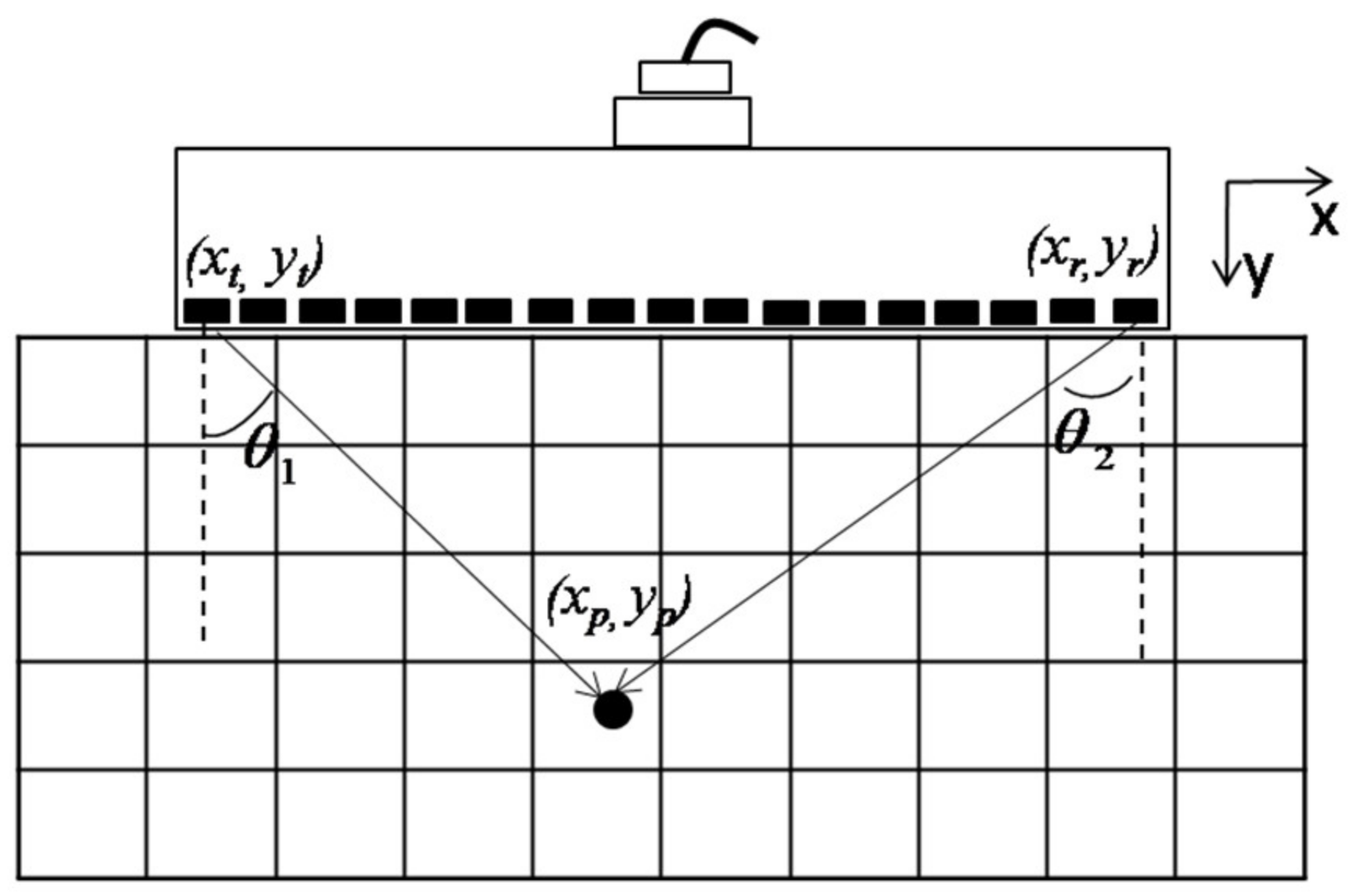
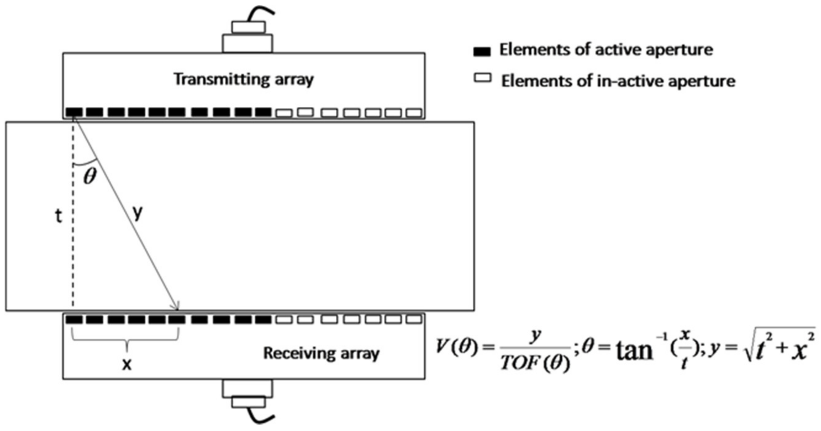
2. FMC/TFM with Anisotropic Velocity Correction

In the FMC-TFM mode, every element in the transducer is fired sequentially, and the individual signals received by all elements (limited by the maximum number of active channels in the instrument) are processed using the TFM algorithm to obtain a focused image in the ROI. The ROI in the inspection medium is divided into grids (pixels), as shown in Figure 1. During TFM processing, the time delays between every transmission-reception pair are calculated for each pixel in the ROI. The time delay corresponding to a pixel is the sum of the time taken for the ultrasonic beam to reach the pixel location (xp, yp) from the transmitter location (xt, yt) and from the pixel location to the receiver location (xr, yr). Once the time delays are calculated, amplitude values corresponding to each transmission–reception pair are obtained by accessing the corresponding individual A-scan signals. In an isotropic material, ultrasonic velocity is constant in all directions. Thus, it is a straightforward method to implement the delay and sum rule for different transmission and reception pairs for the reconstruction of the FMC data to generate a TFM image. However, in the case of an anisotropic material, ultrasonic velocity is direction dependent, and each transmission and reception pair requires individual velocity values to estimate the time delay. Time delay in an anisotropic medium is given by:
T i m e   d e l a y = x t x p 2 + y t y p 2 V θ 1 + x p x r 2 + y p y r 2 V θ 2
where t, p, and r represent the transmitter, pixel, and receiver, respectively. V(θ1) and V(θ2) are the ultrasonic velocities corresponding to beam directions θ1 and θ2 with respect to the surface normal (Figure 1). In the case of an isotropic material, V(θ1) = V(θ2) = V. The angle (θ) varies in a discrete manner with a very small increment. Increment in θ is governed by the size of the pixel in the ROI.
Various approaches have been proposed in the literature to obtain ultrasonic velocities as a function of θ. These include performing measurements in specimens extracted at different angles [27] and performing velocity measurements at different angles by orienting the anisotropic specimen at different angles with respect to the beam directions [28]. Angle-dependent ultrasonic velocities can also be measured by acquiring FMC data in through transmission (TT) mode by using two identical PA probes placed on opposite sides of the specimen, as shown in Figure 2. Different transmitter-receiver combinations correspond to different angles, and by knowing the pitch of the transducers and the thickness of the specimen, distance y and angle θ can be obtained. The velocity values at different angles can then be fitted to a polynomial equation, and the equation can be used to obtain V(θ1) and V(θ2), as required in Equation (1).

3. Experimental Details

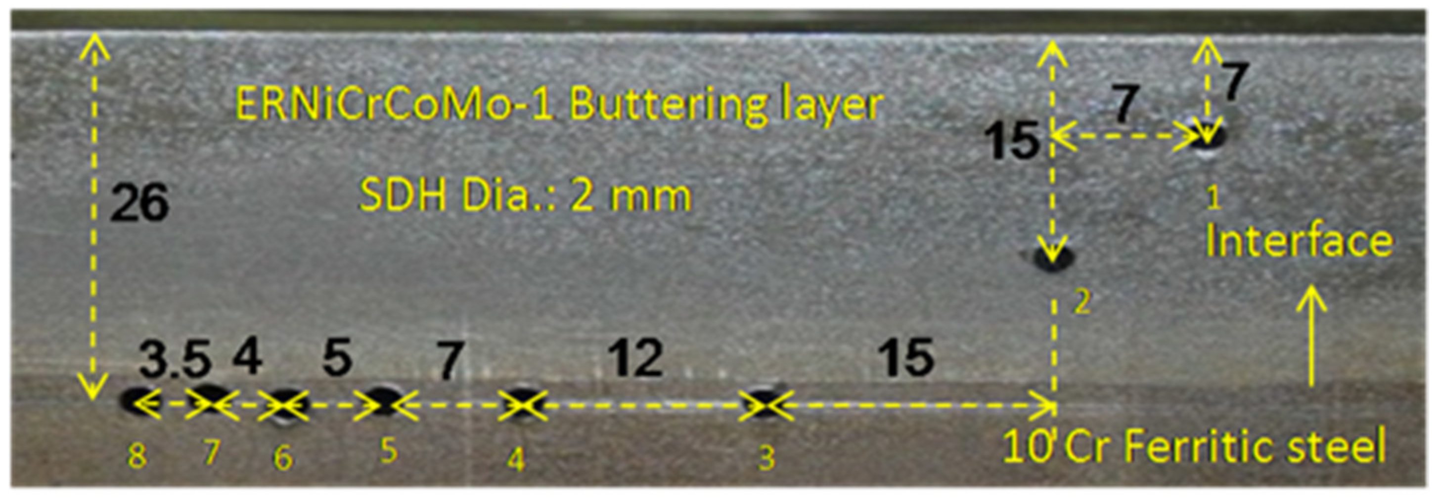
3.1. Specimen Details

Buttering of 200 mm diameter 10Cr steel was carried out by hot-wire TIG welding process using Alloy 617 filler wire (ERNiCrCoMo-1) [4]. The total thickness of the buttering layer was about 25 mm. A sample containing only the buttering layer of about 120 mm length, 25 mm width, and 24 mm thickness was extracted, and the surfaces were made plane parallel for the angle-dependent velocity measurement using the TT mode. Similarly, a sample containing only 10 Cr ferritic steel was also extracted for reference.
Side drilled holes (SDHs) of 2 mm diameter were machined at depths of 7 mm, 15 mm, and 26 mm (near the buttering layer-ferritic steel interface) as reference defects. The photograph of the reference block is shown in Figure 3. The locations of the SDHs in the reference block are also marked in Figure 3.

3.2. Phased Array Ultrasonic Measurements

The experiments were performed using GEKKO© phased array ultrasonic equipment supplied by M/s. Eddyfi, France, with the maximum number of 64 simultaneous transmitting and receiving channels. A 2.25 MHz linear array ultrasonic transducer having 128 elements with an element pitch of 1 mm was used for velocity measurement using the TT technique as well as for defect characterization.
The reason behind selecting the PA probe of 2.25 MHz with 1 mm pitch for the present study is as follows. In a coarse grain material, the material attenuation is primarily governed by grain scattering. The ultrasonic scattering coefficient due to Rayleigh scattering (when λ >> d) can be expressed as:
α s = S d 3 f 4
where S is the scattering factor that depends on the elastic anisotropy and sound velocities, d is the average grain size in the material, and f is the frequency. It can be seen from Equation (2) that the attenuation increases with the fourth power of frequency. In case of a higher frequency, the depth of interrogation is limited, whereas the resolution is improved. It demands a compromise between depth of interrogation and resolution, especially during testing a highly attenuating material [9]. It is always recommended to use a larger aperture to have better resolution. A larger aperture can be achieved either by using a larger pitch or by increasing the number of elements [29]. However, increasing pitch beyond half the wavelength (λ = ~2.4 mm in the present case) may introduce side lobes. Hence, a transducer with 1 mm pitch is used. The data were acquired at 100 MHz and 33.3 MHz sampling frequencies for velocity measurement and defect characterization experiments, respectively. The data for velocity measurements were acquired at the highest available sampling frequency of 100 MHz in the TT mode to obtain the velocity values with the best possible accuracy. However, as longer data lengths are required for defect characterization in pulse-echo and pitch-catch modes, data were acquired at a lower sampling frequency of 33.3 MHz for defect characterization to limit the data file size. The 12-bit data acquired using the GEKKO© system was post-processed using specific software developed in Python.

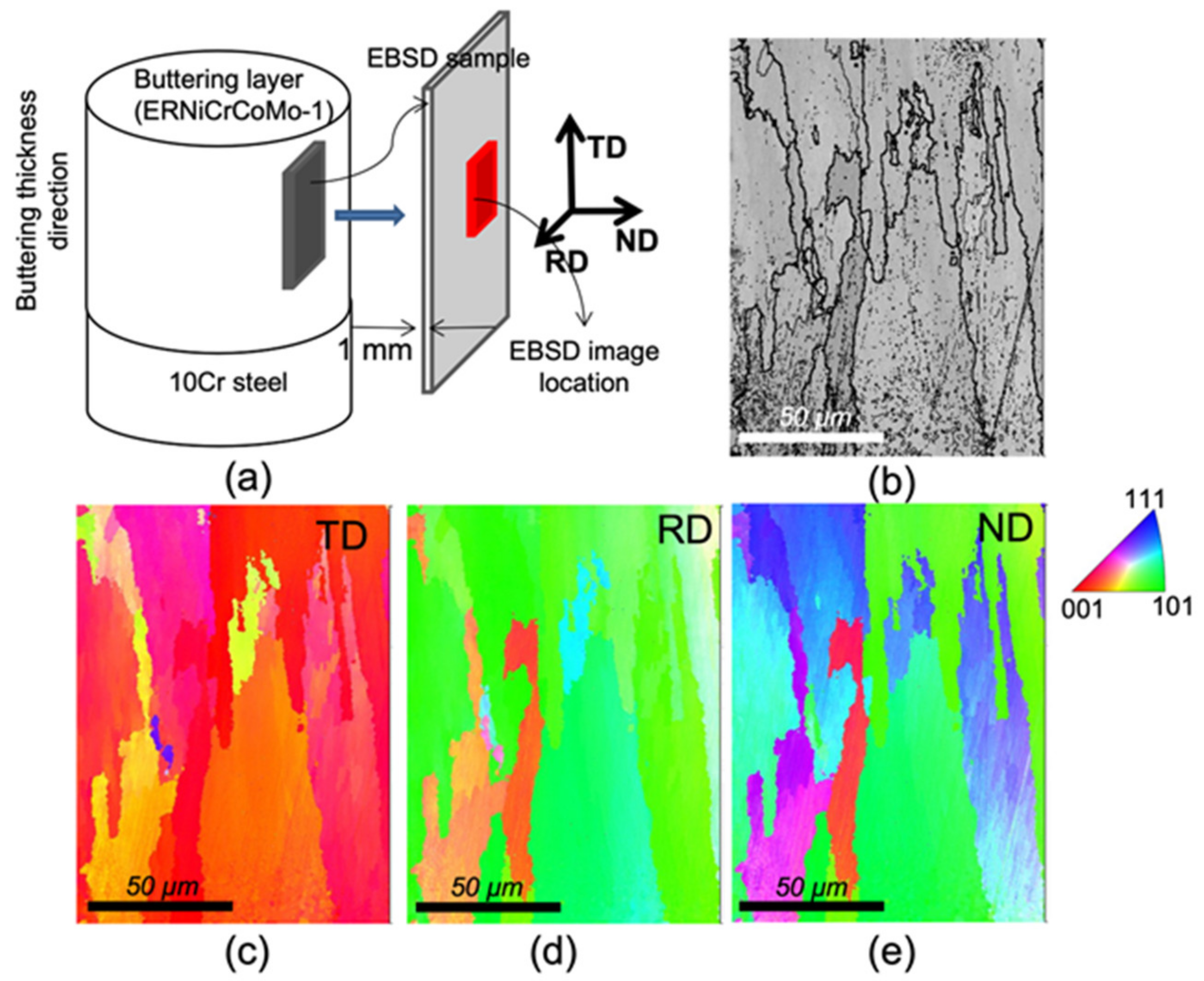
3.3. Electron Back-Scatter Diffraction (EBSD) Study

A sample of size 25 mm (along the buttering thickness direction) × 1 mm (radial) × 5 mm (circumferential) extracted from the alloy 617 buttering layer was used for electron back-scatter diffraction (EBSD) measurements to study the grain orientation. The sample surface was prepared using a conventional metallographic technique up to 0.25 μm diamond polishing. To obtain a stress-free surface, colloidal silica (50 nm) polishing was used. Electron backscatter diffraction (EBSD) studies were performed using a Zeiss SUPRA 55 Gemini field emission gun (FEG) SEM at an accelerating voltage of 20 kV, an aperture of 60 μm and a working distance of 12 mm to obtain the crystallographic orientations to correlate with the angle-dependent ultrasonic velocities.

4. Results and Discussion

4.1. EBSD Results of Grain Orientations

The schematic of the sample extracted for the EBSD study and the EBSD image location in the buttering layer are shown in Figure 4a. The image quality map (Figure 4b) shows the presence of columnar grains elongated in the direction of the buttering thickness (vertical), i.e., perpendicular to the buttering layer-10 Cr steel interface. From the inverse pole figure maps (Figure 4c–e) and the schematic of the sample (Figure 4a), it is observed that the grains are oriented primarily with <100> crystallographic direction along the buttering thickness direction and <110> directions along the radial and the circumferential directions. Similar grain orientations were observed in the specimens extracted from different depths in the buttering deposition direction. These results are in line with those expected for an austenitic alloy to exhibit columnar grain growth along <100> direction perpendicular to the heat extraction plane, here at the buttering layer-10 Cr steel interface [30,31].

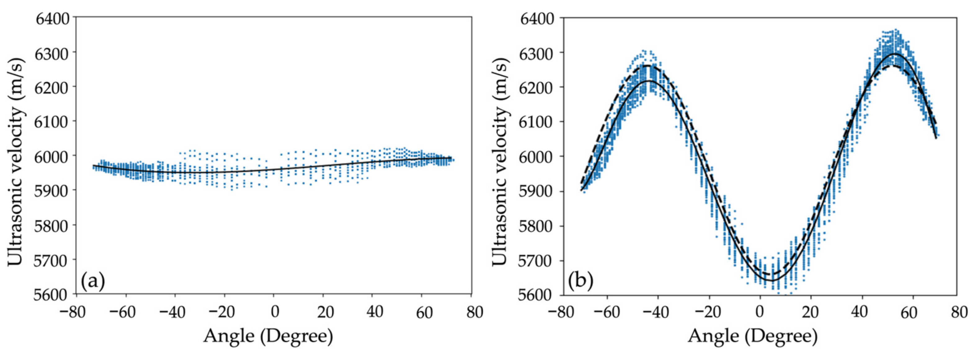
4.2. Angle Dependent Ultrasonic Velocity

In order to validate the phased array TT method for angle-dependent velocity measurement, the method was first applied to a ferritic steel specimen. Then, the same method was adapted to measure angle dependent ultrasonic velocities in the buttering material. Ultrasonic velocity measured using the TT method in the ferritic steel and the buttering layer specimens is shown in Figure 5a,b, respectively. Ultrasonic velocities measured for all 64 transmission and 64 reception conditions, i.e., 64 × 64 velocity values, are shown in Figure 5a,b. For the ferritic steel specimen of thickness ~19.27 mm and 63 mm total aperture of the transducer, velocity values for angles in the range of ±73° are obtained. Similarly, for the buttering layer specimen of ~23.38 mm thickness, velocity values for angles in the range of ±68° are obtained.
The maximum variation in the average ultrasonic velocity with the angle in the ferritic steel specimen is observed to be within about 40 m/s (Figure 5a). However, about 600 m/s variation in the average ultrasonic velocity is observed in the buttering layer (Figure 5b). The average ultrasonic velocity is observed to be minimum (~5650 m/s) at an angle close to 0°, i.e., close to the buttering thickness direction (perpendicular to the buttering layer-10Cr steel interface). Further, the variation in ultrasonic velocity with angle is observed to be almost symmetrical about the vertical plane, i.e., the radial-thickness plane of the buttering. Alloy 617 buttering is a single-phase face-centered cubic (FCC) structure. In an FCC single crystal, the minimum and maximum ultrasonic velocities are expected to be along <100> and <111> directions, respectively, with an intermediate value in the <110> direction [6]. The minimum ultrasonic velocity observed in the direction close to the buttering thickness direction (perpendicular to the interface) is in line with the grain orientation observed by EBSD. Further, a notable variation in ultrasonic velocity is not expected in the depth direction of the buttering layer due to similar grain orientations at different depths.
The variation in ultrasonic velocity with the angle from the buttering thickness direction could be fitted with a sixth-order polynomial as shown by the solid black line in Figure 4b:
V6th(θ) = 5652 − 5.075θ + 0.567θ2 + 0.00369θ3 − 1.64 × 10⁻⁴θ4 − 5.069 × 10⁻⁷θ5 + 1.266 × 10⁻⁸θ6
where θ (in degree) is the angle of the beam propagation direction from the buttering thickness direction in the circumference-thickness plane, and V6th(θ) is the angle dependent velocity in m/s. Further, the velocity profile in the buttering layer in the range of ±68° resembles a sine curve (shown by the dashed black line in Figure 5b), and hence it has also been approximated by a simple equation as given below:
Vsine(θ) = 5960 + 300 × sin(3.75*(θ − 28))
It is to be noted that extrapolations of Equations (3) and (4) beyond ±68° will not provide correct ultrasonic velocities, as ultrasonic velocities at ±90° should be higher than that at 0° due to <110> orientation at 90° and <100> orientation at 0°. However, as the same PA transducer with the same 64-element aperture is also used for defect characterization, the maximum beam angle is limited to ±68° only in the FMC/TFM reconstructions made in this study.

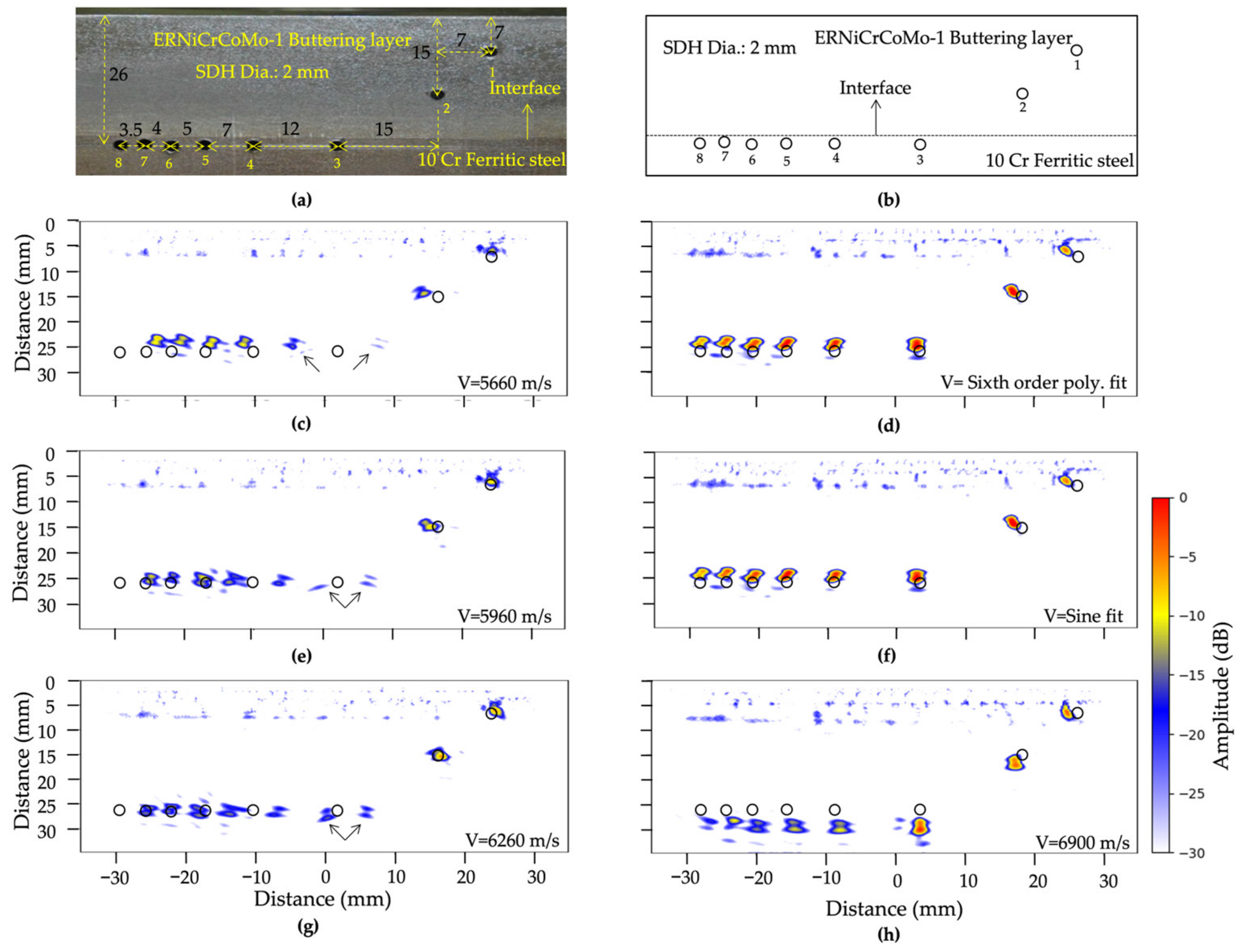
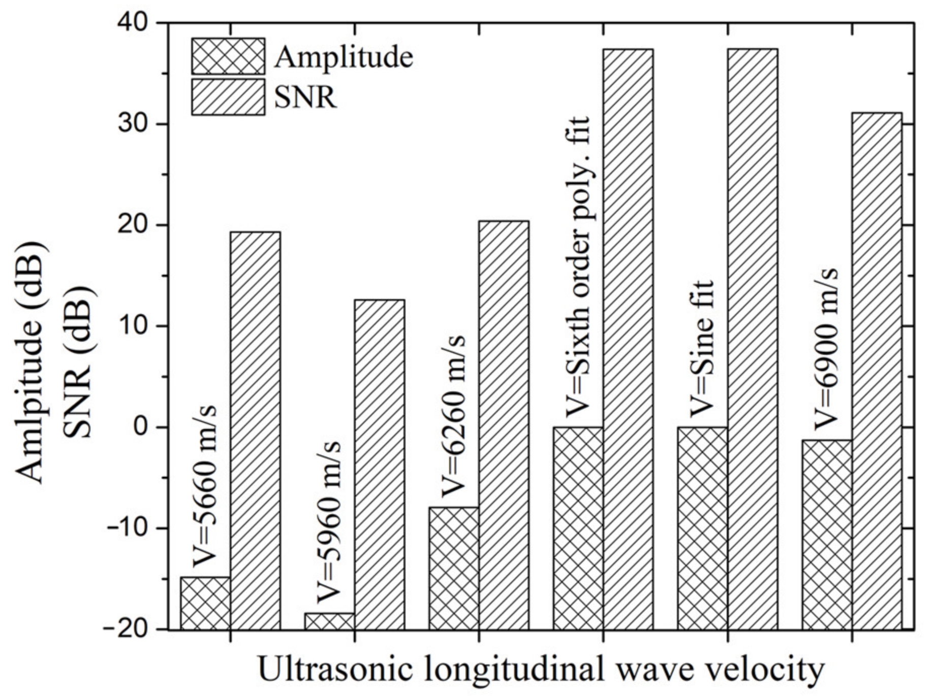
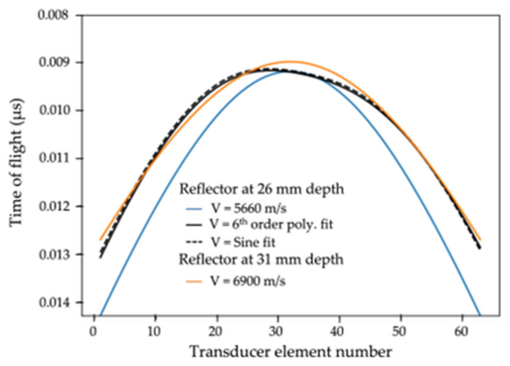
4.3. FMC-TFM Imaging

To study the response of the defects, side drill holes (SDHs) of 2 mm diameter are used as reflectors, as shown in Figure 3. FMC data were acquired with 64-element aperture in 2.25 MHz, 1 mm pitch PA transducer at 33.3 MHz sampling rate. The FMC data were processed using the TFM algorithm developed in Python. Prior to implementing the velocity correction method to the TFM process, the acquired FMC data were processed at different isotropic velocity values. The isotropic velocity values are chosen from the anisotropic velocity curve, as shown in Figure 5b. Those are 5660 m/s, 5960 m/s and 6260 m/s. The velocity values of 5660 m/s and 6260 m/s correspond to the minimum and the maximum in the anisotropic velocity curve, respectively. The 5960 m/s is the average of the two extreme velocities. The TFM images for velocities 5660 m/s, 5960 m/s, and 6260 m/s are shown in Figure 6c,e,g, respectively. The photograph and a schematic sketch of the block with SDHs are shown in Figure 6a,b, respectively, for ready comparison with the FMC-TFM images. All three isotropic velocity cases could image the SDHs at 7 mm and 15 mm depths without any ambiguity. However, the third SDH placed at 26 mm depth exhibited large distortion and splitting. Further, even though only 6 SDHs are present at 26 mm depth, seven indications are observed in Figure 6g, and no indication is observed at the location of the leftmost (8th) SDH in Figure 6c,e,g. This is attributed to the fact that with the isotropic ultrasonic velocities used in these cases in an anisotropic material, TFM reconstructions at different angles do not superimpose at the same point for a given SDH, leading to distorted imaging.
In order to improve the quality of images, TFM images are generated using angle dependent ultrasonic velocities as per Equation (1). The anisotropic velocity corrected TFM images using the sixth order polynomial fit (Equation (3)) and the sine fit (Equation (4)) are shown in Figure 6d,f, respectively. All the SDHs could be effectively reproduced at the corresponding locations in both TFM images with about 6–20 dB improvements in the amplitude for different SDHs as compared to those shown in Figure 6c,e,g. The resolutions obtained at 26 mm depth in these TFM images generated with anisotropic velocity in the buttering layer are observed to be similar to those obtained in isotropic materials at similar depths using similar wavelength and aperture size [29].
Even though TFM images in the anisotropic buttering layer could be obtained with high sensitivity and good resolution by using direction-dependent ultrasonic velocities, this approach cannot be implemented for online inspection using commercial PAUT equipment which provides an option only for a single isotropic ultrasonic velocity to be used for TFM imaging. To enable online inspection with improved FMC/TFM imaging in the anisotropic buttering layer, an alternate approach is proposed. It can be seen in Figure 6c,e,g that the two split indications (marked with arrows) corresponding to the third SDH come closer with an increase in the isotropic ultrasonic velocity used for TFM processing. It is felt intuitively that with a further increase in ultrasonic velocity, the two split indications may overlap to produce a high-amplitude image. Accordingly, TFM images were generated at different ultrasonic velocities above 6260 m/s, even though it is clear that the material does not exhibit ultrasonic velocity above 6260 m/s in any direction in the inspection plane. The TFM image with the highest amplitude of indications for isotropic ultrasonic velocity is obtained at the ultrasonic velocity of 6900 m/s, as shown in Figure 6h. The amplitudes of the first three SDHs in Figure 6h are almost similar to that obtained in Figure 6d,f using angle dependent ultrasonic velocities. However, the amplitudes of the closely spaced SDHs are lower as compared to those in Figure 6d,f. Further, as a higher ultrasonic velocity is used, all the indications are moved at larger depths (29.6 mm) with slight shifts in the lateral positions also.
The effects of isotropic and angle-dependent ultrasonic velocity values on the amplitude and signal-to-noise ratio (SNR), for the third SDH, as observed in Figure 6c–h, are shown in Figure 7. The amplitude values are normalized with respect to that for the same SDH in the TFM image processed with angle dependent velocity obtained using sixth-order polynomial fit. For SNR calculation, the maximum noise amplitude was within 20 mm before the corresponding SDH signal was considered. As seen in Figure 8, the amplitudes and SNRs are similar for the TFM images processed with angle-dependent velocity. Compared to the TFM images processed with the velocity of 5960 m/s (velocity in the isotropic alloy 617), the SNR values for the anisotropy corrected images exhibit about 18 dB higher amplitude and about 25 dB better SNR. Similarly, the alternate approach of using 6900 m/s velocity provided about 18 dB higher amplitude and SNR as compared to that processed with the isotropic velocity of 5960 m/s, exhibiting the efficacy of the methodology.
The reason for obtaining improved imaging at the velocity value of 6900 m/s can be understood from Figure 8. A small reflector is considered at a depth of 26 mm in a buttering layer material. The time of flight (TOF) values calculated for pulse-echo signals received in all elements of a 64-element PAUT transducer of 1 mm pitch kept above the reflector are shown in Figure 8. The TOF values calculated for the angle dependent ultrasonic velocities as per sixth order polynomial fit (Equation (3)) and sine fit (Equation (4)) are shown as solid and dashed black lines. This may be considered as the true TOF values as obtained for the third SDH shown in Figure 6a,b. If a velocity value of 5660 m/s is used, the TOF value matches only at 0°, and a large deviation is observed from the actual values at other angles. In TFM reconstruction, it means that the experimental signals corresponding to most of the elements will not be considered constructively. However, if we use a higher velocity of 6900 m/s and assume the reflector to be at 31 mm depth in an isotropic material, the TOF values (as shown by the orange curve in Figure 8) for most of the elements match closely with that corresponding to the reflector at 26 mm depth in the anisotropic buttering layer. Hence, when the FMC signals obtained from a reflector at a depth of 26 mm in the anisotropic buttering layer are processed using an isotropic velocity of 6900 m/s, a high amplitude well-focused image is observed for the same at ~31 mm depth.
As a single isotropic ultrasonic velocity value is used for generating the TFM image shown in Figure 6h, this can be directly implemented in any commercial PAUT equipment with FMC/TFM facility for obtaining improved imaging in an anisotropic material. The high-velocity value can be considered during real-time testing as a preliminary investigation tool in anisotropic material, and the FMC data can be post-processed using angle dependent ultrasonic velocities for obtaining accurate images. Such an approach will work for other anisotropic materials also (e.g., composites) that exhibit symmetrical anisotropy about the vertical axis in the inspection plane. If the velocity is minimum at 0° and increases with increasing angle (as in the case of the buttering layer), a higher ultrasonic velocity will provide an enhanced image with indications appearing at a larger depth compared to the real depth. Similarly, if the velocity is maximum at 0° and decreases with increasing angle, a lower ultrasonic velocity will provide an enhanced image with indications appearing at a lower depth compared to the real depth.

5. Conclusions

The effect of anisotropic ultrasonic velocity on FMC/TFM image reconstruction is studied in the buttering layer of an austenitic nickel base superalloy (alloy 617). The orientations of the columnar grains with <100> crystallographic direction are observed to be in the buttering thickness direction (perpendicular to the buttering/10Cr steel interface), leading to the minimum Young’s modulus and, thus, the minimum ultrasonic velocity in this direction. The angle dependent ultrasonic velocity measured using a through transmission FMC/TFM approach indicated a variation of about 600 m/s in ultrasonic velocity, with the minimum in the buttering thickness direction (0°) and the maximum at about 50°. The variation in ultrasonic velocity with angles in the range of ±68° from the buttering thickness axis (0°) could be approximated with a simple sine curve.
Splitting of defect indications was observed when the TFM images were generated, considering the buttering layer as an isotropic material having any single value of ultrasonic velocity in the range observed in the buttering layer. This led to reduced sensitivity of defect detection and resolution. The angle dependent ultrasonic velocity could be effectively used for obtaining TFM images with high sensitivity and good resolution. Further, an alternate approach is proposed and demonstrated for obtaining enhanced FMC-TFM imaging in the anisotropic buttering material by using a suitable isotropic velocity much higher than those observed in the material in any direction. The basis of this methodology is also described through suitable simulated conditions. It was found that there is a significant improvement in the SNR of angle-dependent velocity corrected TFM images, and the SNR in the alternate approach is almost close to the angle-dependent velocity corrected TFM images. The alternate approach can be directly implemented in any commercial equipment for improved inspection in an anisotropic material with a symmetrical anisotropy about the thickness axis in the inspection plane.

Author Contributions

Conceptualization, A.K.; methodology, S.P.; software, A.K. and S.P.; validation, S.P.; formal analysis, S.P., A.K. and K.V.R.; data curation, S.P.; writing—original draft preparation, S.P.; writing—review and editing, A.K. and K.V.R.; visualization, S.P.; supervision, A.K. All authors have read and agreed to the published version of the manuscript.

Funding

This research received no external funding.

Institutional Review Board Statement

Not applicable.

Informed Consent Statement

Not applicable.

Data Availability Statement

The data presented in this study are available on request from the corresponding author. The data are not publicly available due to restrictions.

Acknowledgments

Authors are thankful to Harish Chandra Dey, Head, Advanced Materials Fabrication Section for providing the sample with the buttering layer and Vani Shankar, Head, Fatigue Studies Section for the EBSD studies. Authors are also thankful to John Philip, Materials Characterization and Engineering Group, and R. Divakar, Metallurgy and Materials Group for their encouragement and support.

Conflicts of Interest

The authors declare no conflict of interest.

References

  1. Chetal, S.C.; Jayakumar, T.; Bhaduri, A.K. Materials Research and Opportunities in Thermal (Coal-based) Power Sector Including Advanced Ultra Super Critical Power Plants. Proc Indian Natl. Sci. Acad. 2015, 81, 739–754. Available online: http://scinet.science.ph/union/Downloads/Vol81_2015_4_Art06_336304.pdf (accessed on 4 March 2023). [CrossRef]
  2. Ahmad, H.W.; Hwang, J.H.; Lee, J.H.; Bae, D.H. An Assessment of the Mechanical Properties and Microstructural Analysis of Dissimilar Material Welded Joint between Alloy 617 and 12Cr Steel. Metals 2016, 6, 242. [Google Scholar] [CrossRef]
  3. Bhatt, N.C.; Batrani, M.; Mohan, J.; Gopalakrishnan, V.; Verma, M.K. Challenges in Design and Development of Steam Turbine Rotors with Alloy 617(M) for Indian AUSC Program. Int. J. Eng. Res. Technol. 2019, 8, 139–143. Available online: https://www.ijert.org/research/challenges-in-design-and-development-of-steam-turbine-rotors-with-alloy617m-for-indian-ausc-program-IJERTV8IS010068.pdf (accessed on 4 March 2023).
  4. Sakthivel, T.; Dey, H.C.; Parida, P.K.; Prasad Reddy, G.V.; Vasudevan, M.; Albert, S.K. Integrity Assessment of 10Cr Ferritic Steel/Alloy 617M Dissimilar Metal Weld Joint under Creep Condition. J. Mater. Eng. Perform. 2023, (in press). [Google Scholar] [CrossRef]
  5. Temple, J.A.G. Modelling the propagation and scattering of elastic waves in homogeneous anisotropic elastic media. J. Phys. D Appl. Phys. 1988, 21, 859–874. [Google Scholar] [CrossRef]
  6. Kupperman, D.S.; Reimann, K.J. Efect of shear-wave polarization on defect detection in stainless steel weld metal. Ultrasonic 1978, 16, 21–27. [Google Scholar] [CrossRef]
  7. Tomlinson, J.R.; Wagg, A.R.; Whittle, M.J. Ultrasonic inspection of austenitic welds. Br. J. Non-Destr. Test. 1980, 22, 119–127. [Google Scholar]
  8. Lhuillier, P.E.; Chassignole, B.; Oudaa, M.; Kerhervé, S.O.; Rupin, F.; Fouquet, T. Investigation of the ultrasonic attenuation in anisotropic weld materials with finite element modeling and grain-scale material description. Ultrasonics 2017, 78, 40–50. [Google Scholar] [CrossRef]
  9. Kumar, A.; Arnold, W. High resolution in non-destructive testing: A review. J. Appl. Phys. 2022, 132, 100901. [Google Scholar] [CrossRef]
  10. Hudgell, R.; Gray, B. The Ultrasonic Inspection of Austenitic Materials: State of the Art Report; OECD Nuclear Energy Agency: Oxfordshire, UK, 1985; Available online: https://www.oecd-nea.org/upload/docs/application/pdf/2020-01/csni85-94.pdf (accessed on 4 March 2023).
  11. Takasawa, K.; Miki, K. Development of High and Intermediate Pressure Steam Turbine Rotors for Efficient Fossil Power Technology. Available online: https://www.jsw.co.jp/news/news_file_division/file/File024476424.pdf (accessed on 4 March 2023).
  12. Baiotto, R.; Gregson, B.K.; Nageswaran, C.; Clarke, T. Coherence Weighting Applied to FMC/TFM Data from Austenitic CRA Clad Lined Pipes. J. Nondestruct. Eval. 2018, 37, 49. [Google Scholar] [CrossRef]
  13. Cunningham, L.J.; Mulholland, A.J.; Tant, K.M.M.; Gachagan, A.; Harvey, G.; Bird, C. The detection of flaws in austenitic welds using the decomposition of the time-reversal operator. Proc. R. Soc. A 2016, 472, 20150500. [Google Scholar] [CrossRef] [PubMed]
  14. Metwally, K.; Lubeigt, E.; Rakotonarivo, S.; Chaix, J.F.; Baqué, F.; Gobillot, G.; Mensah, S. Weld inspection by focused adjoint method. Ultrasonics 2018, 83, 80–87. [Google Scholar] [CrossRef] [PubMed]
  15. Long, R.; Russell, J.; Cawley, P. Ultrasonic phased array inspection using full matrix capture. Insight-Non-Destr. Test. Cond. Monit. 2012, 54, 380–385. [Google Scholar] [CrossRef]
  16. Ye, J.; Kim, H.J.; Song, S.J.; Kang, S.S.; Kim, K.; Song, M.H. Model-based simulation of focused beam fields produced by a phased array ultrasonic transducer in dissimilar metal welds. NDTE Int. 2011, 44, 290–296. [Google Scholar] [CrossRef]
  17. Russell, J.; Long, R.; Duxbury, D.; Cawley, P. Development and implementation of a membrane-coupled conformable array transducer for use in the nuclear industry. Insight-Non-Destr. Test. Cond. Monit. 2012, 54, 386–393. [Google Scholar] [CrossRef]
  18. Holmes, C.; Drinkwater, B.W.; Wilcox, P.D. Post-processing of the full matrix of ultrasonic transmit–receive array data for non-destructive evaluation. NDTE Int. 2005, 38, 701–711. [Google Scholar] [CrossRef]
  19. Zhou, H.; Han, Z.; Du, D.; Chen, Y. A combined marching and minimizing ray-tracing algorithm developed for ultrasonic array imaging of austenitic welds. NDT E Int. 2018, 95, 45–56. [Google Scholar] [CrossRef]
  20. Kolkoori, S.R.; Rahman, M.U.; Chinta, P.K.; Ktreutzbruck, M.; Rethmeier, M.; Prager, J. Ultrasonic field profile evaluation in acoustically inhomogeneous anisotropic materials using 2D ray tracing model: Numerical and experimental comparison. Ultrasonics 2013, 53, 396–411. [Google Scholar] [CrossRef]
  21. Nowers, O.; Duxbury, D.J.; Drinkwater, B.W. Ultrasonic array imaging through an anisotropic austenitic steel weld using an efficient ray-tracing algorithm. NDTE Int. 2016, 79, 98–108. [Google Scholar] [CrossRef]
  22. Kim, H.H.; Kim, H.J.; Song, S.J.; Kim, K.C.; Kim, Y.B. Simulation Based Investigation of Focusing Phased Array Ultrasound in Dissimilar Metal Welds. Nucl. Eng. Technol. 2016, 48, 228–235. [Google Scholar] [CrossRef]
  23. Li, C.; Pain, D.; Wilcox, P.D.; Drinkwater, B.W. Imaging composite material using ultrasonic arrays. NDTE Int. 2013, 53, 8–17. [Google Scholar] [CrossRef]
  24. Sumana; Kumar, A. Phased array ultrasonic imaging using angle beam virtual source full matrix capture-total focusing method. NDTE Int. 2020, 116, 102324. [Google Scholar] [CrossRef]
  25. Tant, K.M.M.; Mulholl, A.J.; Galetti, E.; Curtis, A.; Gachagan, A. Mapping the Material Microstructure of Safety Critical Components Using Ultrasonic Phased Arrays. In Proceedings of the IEEE International Ultrasonics Symposium (IUS), Tours, France, 18–21 September 2016; pp. 1–4. [Google Scholar] [CrossRef]
  26. Harvey, G.; Tweedie, A.; Carpentier, C.; Reynolds, P. Finite element analysis of ultrasonic phased array inspection of anistropic welds. AIP Conf. Proc. Rev. Prog. Quant. Nondestruct. Eval. 2011, 30, 827–834. [Google Scholar] [CrossRef]
  27. Ploix, M.A.; Guy, P.; Chassignole, B.; Moysan, J.; Corneloup, G.; Guerjouma, R.E. Measurement of ultrasonic scattering attenuation in austenitic stainless steel welds: Realistic input data for NDT numerical modelling. Ultrasonics 2014, 54, 1729–1736. [Google Scholar] [CrossRef]
  28. Hurley, D.C.; Fitting, D.W.; Chiao, R.Y. Angularly-dependent ultrasonic velocity and attenuation measurements in an anisotropic material. Rev. Prog. Quant. Nondestr. Eval. 1995, 14A, 1585–1592. [Google Scholar]
  29. Sumana; Kumar, A. Parametric Study on Resolution Achieved Using FMC-TFM-Based Phased Array Ultrasonic Imaging. In Advances in Non-Destructive Evaluation. Lecture Notes in Mechanical Engineering; Mukhopadhyay, C.K., Mulaveesala, R., Eds.; Springer: Singapore, 2021. [Google Scholar] [CrossRef]
  30. Mark, A.F.; Fan, Z.; Azough, F.; Lowe, M.J.S.; Withers, P.J. Investigation of the elastic/crystallographic anisotropy of welds for improved ultrasonic inspections. Mater. Charact. 2014, 98, 47–53. [Google Scholar] [CrossRef]
  31. Tabatabaeipour, S.M.; Honarvar, F. A comparative evaluation of ultrasonic testing of AISI 316L welds made by shielded metal arc welding and gas tungsten arc welding processes. J. Mater. Process. Technol. 2010, 210, 1043–1050. [Google Scholar] [CrossRef]
Figure 1. Schematic of TFM methodology.
Applsci 13 05195 g001
Figure 2. Schematic showing the phased array trough-transmission (TT) setup used for measuring angle-dependent anisotropic ultrasonic velocity.
Applsci 13 05195 g002
Figure 3. Photograph of the reference block used in the present study. The depths of the side drill holes (SDHs) and their relative distances are given in mm.
Applsci 13 05195 g003
Figure 4. EBSD images and grain orientation: (a) schematic of the sample extracted for the EBSD study and EBSD image location in the buttering layer, (b) image quality map, and (ce) inverse pole figure (IPF) maps corresponding to the buttering thickness, circumferential and radial directions, respectively.
Applsci 13 05195 g004
Figure 5. Variations in ultrasonic longitudinal wave velocity with the angle from the surface normal for: (a) the ferritic steel; (b) the buttering layer.
Applsci 13 05195 g005
Figure 6. (a) Photograph and (b) schematic sketch of the reference block showing locations of side drill holes (SDHs). (c,e,g) are TFM images processed using isotropic ultrasonic longitudinal wave velocity values of 5660 m/s, 5960 m/s, and 6260 m/s, respectively. (d,f) provide TFM images generated using angle dependent ultrasonic velocities as per the sixth-order polynomial fit (Equation (3)) and the sine fit (Equation (4)), respectively. (h) TFM image generated using the alternate approach with an isotropic ultrasonic velocity of 6900 m/s. The amplitude values in dB scale for all the TFM images are calculated with respect to the maximum amplitude observed in (d).
Applsci 13 05195 g006
Figure 7. Amplitude and signal-to-noise ratio (SNR) obtained for third SDH in the TFM images processed with isotropic and angle dependent ultrasonic velocity values as shown in Figure 6. The amplitude values are normalized with respect to that of the same SDH in the TFM image processed with angle dependent velocity obtained using sixth-order polynomial fit.
Applsci 13 05195 g007
Figure 8. Variations in calculated time of flight values for 64 elements configurations working in pulse-echo mode.
Applsci 13 05195 g008
Disclaimer/Publisher’s Note: The statements, opinions and data contained in all publications are solely those of the individual author(s) and contributor(s) and not of MDPI and/or the editor(s). MDPI and/or the editor(s) disclaim responsibility for any injury to people or property resulting from any ideas, methods, instructions or products referred to in the content.

