Article

Rapid Parametric Modeling and Robust Analysis for the Hypersonic Ascent Based on Gap Metrics

College of Astronautics, Nanjing University of Aeronautics and Astronautics, Nanjing 211106, China
*
Author to whom correspondence should be addressed.
Appl. Sci. 2023, 13(8), 5189; https://doi.org/10.3390/app13085189
Submission received: 27 March 2023 / Revised: 16 April 2023 / Accepted: 18 April 2023 / Published: 21 April 2023
(This article belongs to the Special Issue Advanced Guidance and Control of Hypersonic Vehicles)

Abstract

:
This paper investigates a rapid modeling method and robust analysis of hypersonic vehicles using multidisciplinary integrated techniques. First, the geometrical configuration is described using parametric methods based on the class–shape technique. Aerodynamic forces and moments are estimated for the specific configuration using engineering methods. Moreover, the nonlinear model is simplified by the polynomial fitting expressions, and the linear variable parameter model is obtained for the tracking control design and dynamic characteristic analysis with the aid of the sensitivity analysis and gap metric methods. A velocity-driven trajectory design method is deduced for hypersonic ascent, and the tracking control law is developed to realize the flight process from the initial point to the cruise point. Furthermore, a robust analysis process based on gap margin is proposed for climb trajectory tracking. Simulation results are provided to verify the feasibility of the proposed modeling method and show that the flight control of a hypersonic vehicle is more sensitive to altitude variation.

1. Introduction

Reusable hypersonic flight vehicles for future aerospace access will dramatically improve economy and efficiency [1]. However, such aerospace vehicles must pass through the large flight envelope from subsonic flight to hypersonic, leading to unexpected dynamic features compared with other traditional vehicles. Hence, researchers on hypersonic aerospace vehicles need to adopt a multidisciplinary integrated strategy concerning the propulsion system, aerodynamics, control, and structural dynamics [2].
The parametric modeling approach offers a favorable way for the aerospace vehicle to implement the multidisciplinary integrated design [3]. In particular, an analytical aeropropulsive/aeroelastic aerospace vehicle model was established [4], and the model involves a two-dimensional aerodynamic structure, a one-dimensional SCRAMjet-type propulsion system, and an elastic airframe [5]. Alternatively, a nonlinear longitudinal dynamical model was derived from first principles, capturing inertial coupling effects between the propulsion system, aerodynamics, and structural dynamics [6,7]. Furthermore, a control-oriented model of the aerospace vehicle was obtained in [8] by replacing complex force and moment equations with curve-fitted approximations, and this model allows an understanding of the applicability of control-oriented techniques. In addition, a 3D simulation model of the aerospace vehicle was built [9], and intrinsic flexibility was considered with a one-dimensional Euler–Bernoulli beam representation. This model was subjected to stability analysis and control-based design. However, some problems still need to be addressed to enhance the overall performance, including the integrated design of the trajectory and vehicle shape, control-centric trade study, and multidisciplinary design optimization.
Additionally, the control-centric trade studies were conducted based on a parametric model, and this work explores the parameterization types, parameter ranges, and objectives available for the analysis and optimization of the aerospace vehicle [10]. Moreover, a multidisciplinary optimization method was proposed [11], and the optimal vehicle configuration and flight trajectory are determined to accomplish the mission requirements. The parametric model provides a suitable way to change a vehicle optimized for a single design point to be more effective along a trajectory [12]. In summary, the parametric model is a fundamental issue for further studies. Furthermore, the model provides an effective tool to construct the mutual relations between the propulsion, aerodynamics, control, and structural dynamics so that the optimal trade results for the aerospace vehicle design can be easily obtained in the conceptual stage.
Some control-relevant issues are revealed for hypersonic flight based on these proposed models [13], including the coupled features of the plant and trajectory [14]. In addition, hypersonic flight suffers from control system constraints, which limits the performance for trajectory tracking [15]. Moreover, the robustness of flight control is particularly significant on account of the uncertainty of the model and environment. Many robust control design methods have been developed [16,17,18]. Their works focused on the development of a nonlinear adaptive robust control method to deal with model uncertainty. However, few methods have been proposed for quantifying the robustness of the flight control system. A robust analysis method based on a gap metric is proposed in this paper. The benefit of the proposed method is the quantitative analysis ability to identify the boundary of the robustness, whereas the drawback is the restriction from the nonlinear system. One has to formulate a series of linearized systems to approximate the nonlinearity.
The structure of the paper is organized as follows. Section 1 introduces the model of aerospace vehicles and deduces the polynomial fitting model of longitudinal dynamics for the following control design. A linear parameteric varying model is driven based on a gap metric in Section 2. Then, a velocity-driven method is proposed to solve the optimal ascent problem and a robust analysis method based on gap margin is proposed to qualify the closed-loop performance. Furthermore, the simulation results are provided and discussed in Section 4.

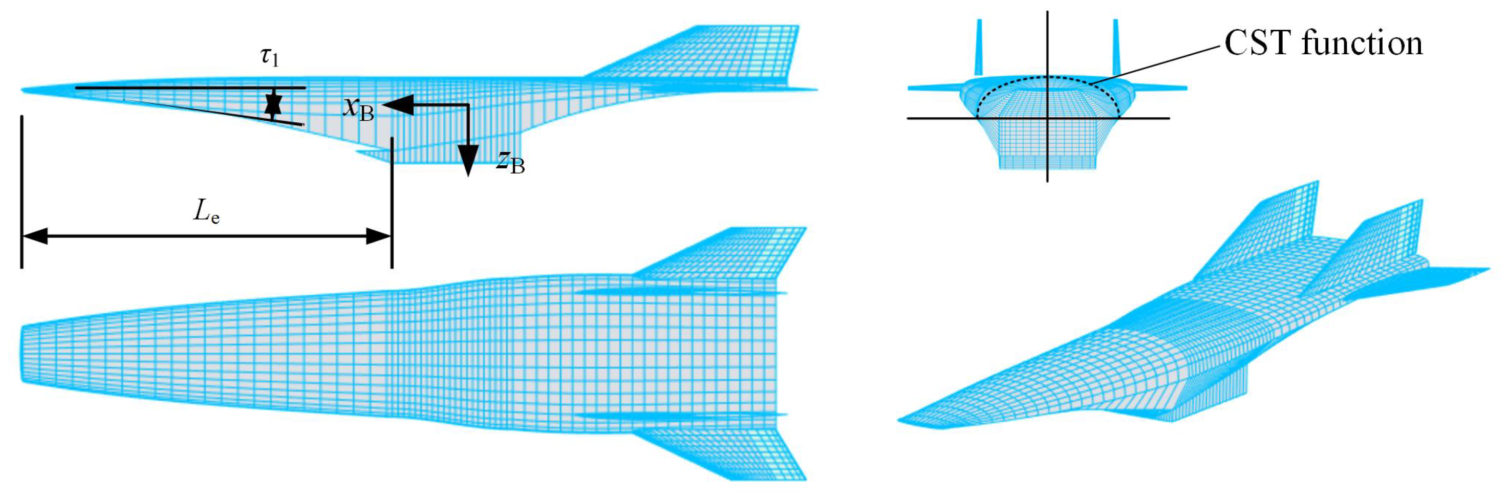
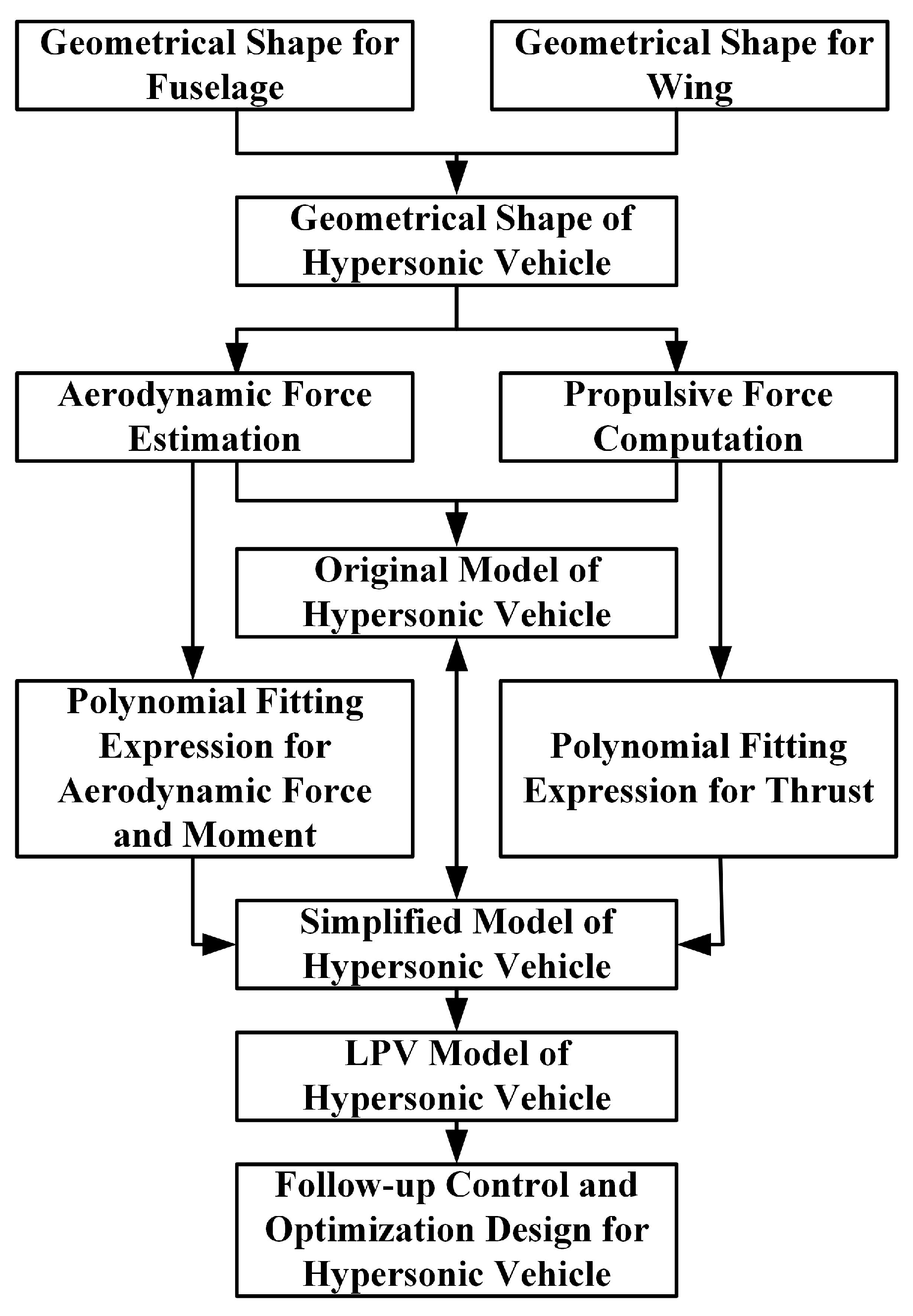
2. Model Description

In this paper, the parametric keel-line is firstly formulated based on the second-order curve method, and then the section along with the body x-axis x is identified using the “shape function/class function” transformation (CST) technique [19]. To this end, the geometrical configuration of the aerospace vehicle is divided into two classes: the fuselage and wing. In particular, the fuselage shape is considered to be the stretching results of the profile curve for the body axis x B , and thus the fuselage design needs to first determine the relevant equation of each profile curve.
Afterward, the relations of the profile parameters along with the body axis need to be determined according to the top, bottom, and front view. Aside from the fuselage, the wing is considered to be a flat plate with variable thickness [20]. In addition, the installation position of the wing has a significant impact on the control capacity. As a result, the relative position of the leading edge from the fuselage to the wing, the relative position from the wing’s leading edge to the bottom of the vehicle, and the wing mounting angle are selected as the main parameters to describe the wing placement.
The aerospace vehicle adopts an integrated structure such that the airframe and the engine are changed into a whole. That is, the outer surface of the engine is treated as a part of the fuselage. Thus, the internal geometry structure will affect the thrust. Typically, the engine configuration is considered to be a ladder tube with a variable area including five parts: the inlet part, intake part, isolation section, combustion chamber, and internal nozzle [21]. In principle, the inlet is designed as the ladder tube with variable area to make the airflow compressed; the isolation section is given as the ladder tube with the same area to suppress the unfavorable effect on the inlet due to the combustion; the internal nozzle is considered to be the ladder tube with variable area when the airflow is expanded. Furthermore, the given parameters associated with the fuselage, aerofoil, and engine are interrelated as a result of the fact that the constrained relations need to be identified to construct the complete configuration. To this end, the configuration of the aerospace vehicle is built in Figure 1.

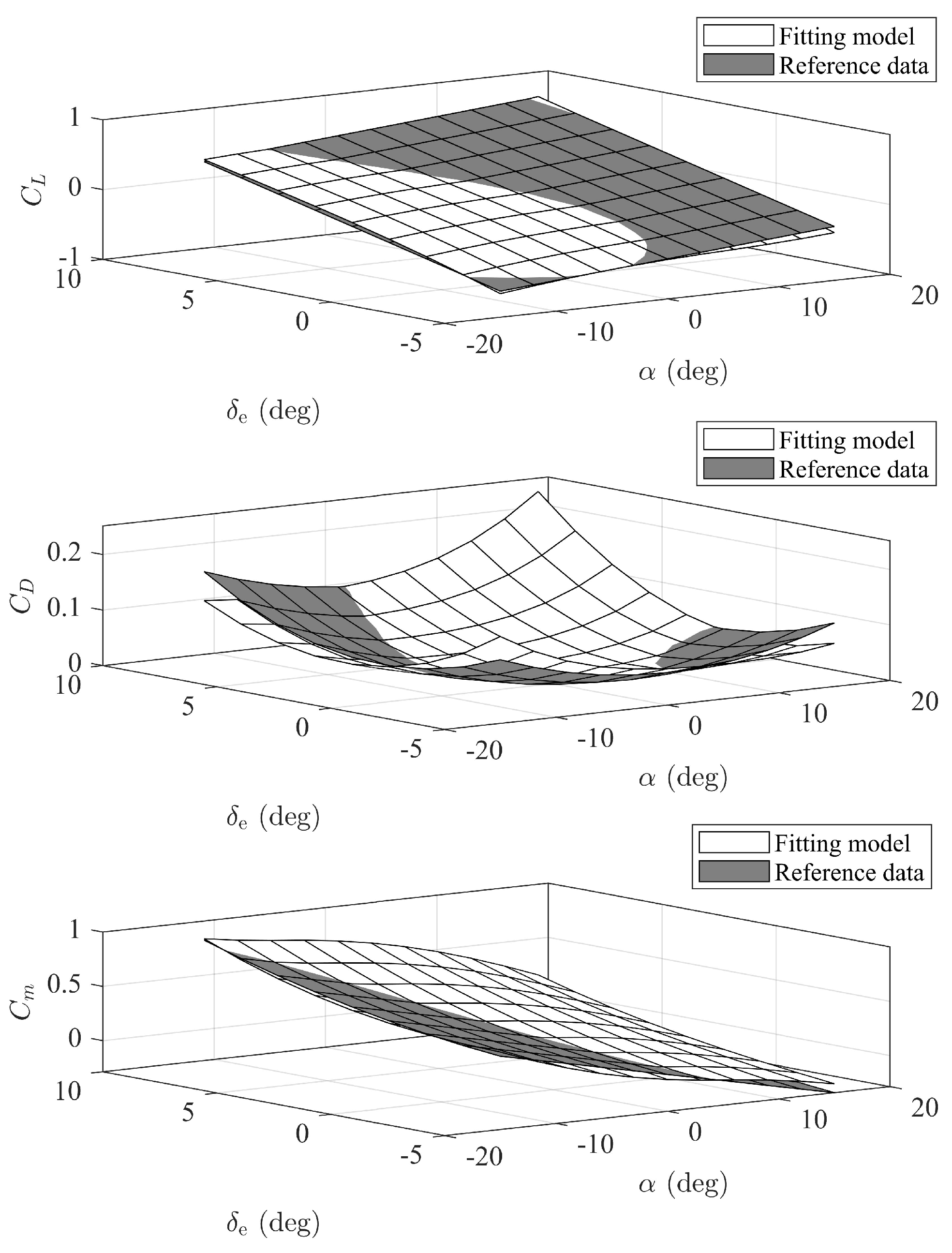
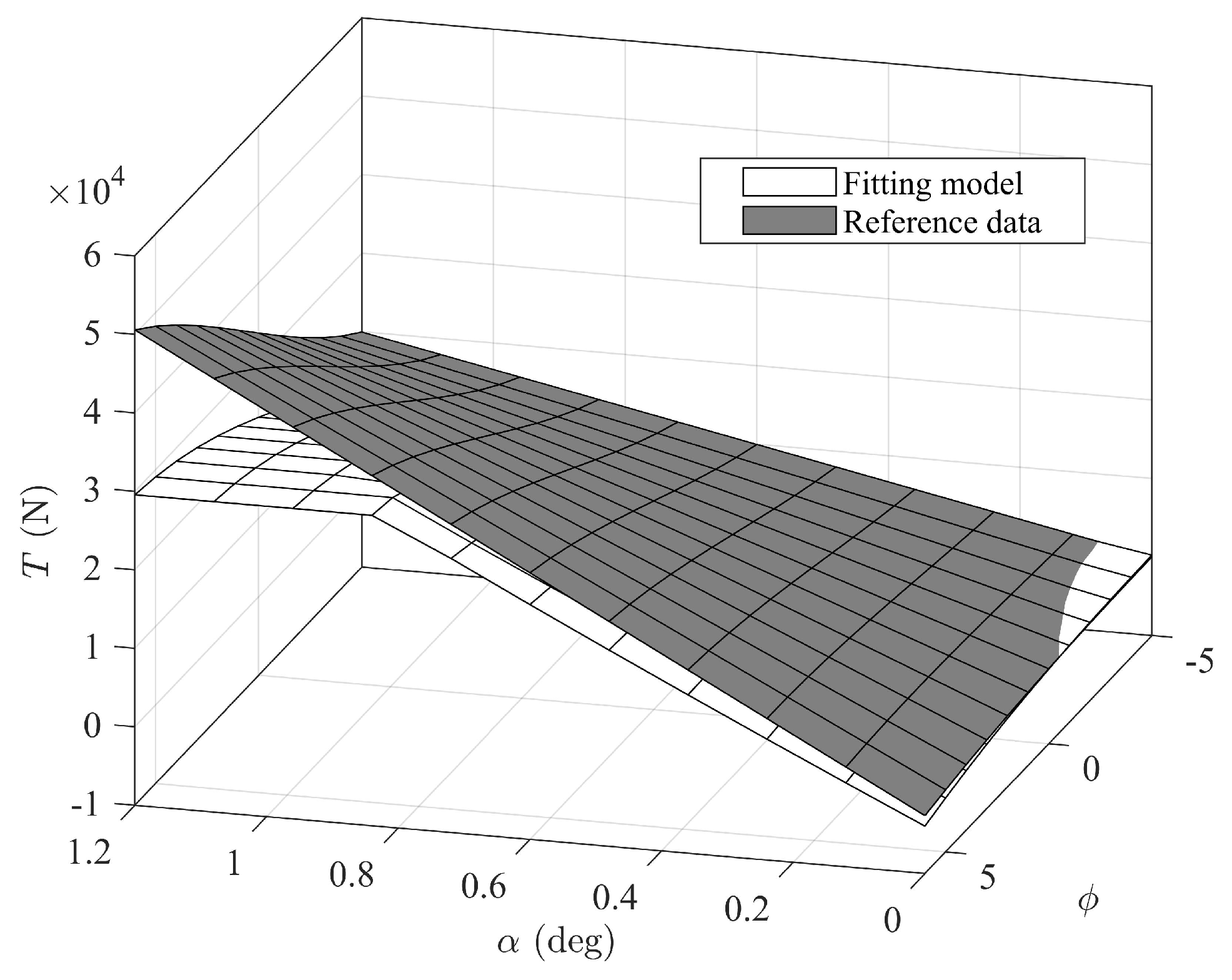
2.1. Force Estimation

As soon as the configuration of the aerospace vehicle is identified, the following task is to acquire the forces for establishing the dynamic model. In this article, we divide the vehicle body into several surface elements, considered the triangle surface [22]. For each surface element in the face of freeflow, the oblique shock theory is used to estimate the enforced pressure coefficient C p , and it is expressed by [23]
C p = 4 γ c + 1 ( sin 2 β s 1 M a 2 )
where γ c denotes the specific heat ratio; M a is the flight Mach number; and β s is the shock wave angle, which is solved based on the flow turning angle δ by the following equation:
tan δ = 2 cot β s · M a 2 sin 2 β s 1 M a 2 γ c + cos 2 β s + 2
Alternatively, if the surface element lies on the leeward side, the Prandtl–Meyer theory is adopted to estimate the pressure coefficient, which is calculated by [24]
C p = 2 γ c M a u 2 1 + γ c 1 2 M a u 2 1 + γ c 1 2 M a d 2 γ c γ c 1 1
where the subscripts u and d denote the parameters before and after the shock wave, respectively, which are solved based on the flow turning angle by
δ = ν M a d ν M a u
where ν ( M a ) is the Prandtl–Meyer function.
Once the pressure coefficient is obtained for the surface element, the suffered pressure is computed by
P i = C p i s a , i + P
where P denotes the static pressure, and s a , i denotes the area of the i-th surface element. The aerodynamic forces and moments are yielded by superimposing these pressures for all surface elements, and they are expressed by [25]
F x = P i n x i S i F y = P i n y i S i F z = P i n z i S i
M x = P i ( r z i n y i r y i n z i ) S i M y = P i ( r x i n z i r z i n x i ) S i M z = P i ( r y i n x i r x i n y i ) S i
where r i = r x i e x + r y i e y + r z i e z represents the distance vector from the vehicle centroid to the center of each surface element.
Aside from aerodynamic forces, the thrust is calculated using the momentum theorem, and it is expressed by [26]
F T = m ˙ a [ ( 1 + f s t ) V 5 V 1 ] + ( P 5 P 1 ) A e ( P 2 P 1 ) A 1
where m ˙ a denotes the air flow rate; ϕ is the stoichiometric ratio; f s t represents the stoichiometric fuel–air ratio; V 1 and P 1 indicate the airflow parameters at the inlet; V 5 and P 5 denote the airflow parameters at the nozzle; A e and A 1 are the areas in relation to the nozzle exit plane and inlet plane, respectively; P 2 represents the pressure of the compressed section.
Furthermore, the pitching moment induced by the propulsive force is expressed by
M T = r T G × F T
Similar to the aerodynamic coefficient, the thrust coefficient and propulsive moment coefficient are formulated by
C T = 2 F T ρ V 2 S cap
where S cap denotes the capture area of the engine and ρ indicates freeflow density.

2.2. Longitudinal Dynamics

The longitudinal dynamic equation of the aerospace vehicle in the air flow coordination is established as follows [27]:
h ˙ = V sin θ α V ˙ = F T cos α D m g sin θ α α ˙ = F T sin α L m V + q + g V cos θ α θ ˙ = q q ˙ = 1 I y M y
where h denotes the flight altitude, V is the flight velocity, α is the angle of attack (AOA), θ is the pitch angle, and q is the pitch angle rate. g is the gravity constant; m and I y denote the mass and moment of inertia of the aerospace vehicle, respectively. In addition, L, D, and M y denote the lift, drag, and pitch moment, respectively. The forces and moments are estimated by the methods described above, and the mechanical properties should be further analyzed for control system design.

2.3. Polynomial Fitting Modeling

The mechanical model based on the finite element method is very complicated for implementing the control design and integrated optimization for the aerospace vehicle. Hence, the surrogate models of the aerodynamic forces and moments need to be first acquired, and they are expressed by [28]
L = q ¯ S ref C L D = q ¯ S ref C D F T = q ¯ S cap C T M y = q ¯ S ref l ref C m + z T F T
where q ¯ is the dynamic pressure, and S ref and l ref are the reference area and length, respectively. z T is the shift of the thrust axis from the center of gravity.
Furthermore, the polynomial fitting method is applied to identify the specific forms concerning C L , C D , C T , and C m . The surrogate procedure consists of four steps: the design of the sample points, selection of the model structure, identification of the model parameters, and verification of the acquired model. Without loss of generality, we first select y = C L as the identification parameter to expatiate this design course.
The sampling points for C L are constructed using the Latin hypercube sampling method with the subsequent evaluation criterion:
E e = i = 1 N j = i + 1 N 1 x i x j 2
where N is the number of the sample points; x i and x j denote the positions of the i-th and j-th sample points.
In principle, the selected sample points can ensure that the distance among the sample points is the maximum, matching the minimum evaluation criterion of (14). According to these obtained sample points, we consider further the surrogate model (SM) of C L with the following form:
y = f A cof , x
where A cof denotes the contingent coefficients which need to be determined in terms of the trust region method. Furthermore, we define the residual errors as
Δ y = min A cof f A cof , x y obs 2 2
where y obs denotes the outputs of the sample points. In particular, the SM is comprised of first-degree terms, quadratic terms, and two crossing terms. However, such polynomial items complicate the iterative computation for obtaining these contingent coefficients. Therefore, the optimum selection of these items aids in simplifying the modeling courses.
In this paper, a sensitivity analysis method is adopted to choose the identified items, and this method is based on the iterative fractional factorial design (IFFD), which distinguishes the influence relation between outputs and inputs.
The basic design matrix of FFD with k parameters is donated as J n i , columns of which represent the sampling level of parameters. The orientation of an iteration is defined as positive, negative, or null. A positive orientation means the sampling values of the parameter agree with the notation of the basic design matrix (high: +1, low: −1), while negative means the opposite, and null represents sampling at the median 0.
The procedure of IFFD consists of two steps of randomization [13]. The first step affects the whole set of iterations. The orientation of each iteration is randomized with a specified proportion of null orientation. The random direction matrix O n k is identified. The parameters are randomly assigned to columns of the basic design matrix J n i and generate the new basic design matrix J n i . After that, the sampling matrix Q k and response matrix Y k = y are determined for the k-th iteration wherein Q k is expressed by
Q k = J n i · d i a g O n k : , k
For IFFD screening analysis, one must simulate the experiments according to the sampling matrix. The main effect of the i-th parameter is identified by the difference in average response between the two levels (1 and −1), which is assumed to be a linear effect:
M E i , Y = k = 1 n k Q k : , i Y k k = 1 n k O k i , k
The analysis of the interaction effect of parameters is similar to the main effect. Nonlinear effects of the i-th parameter are identified by the difference in average response between the median (0) and the boundary (1, −1), which is assumed to be a quadratic effect:
M E i , Y = k = 1 n k j = 1 2 n i 1 Q k j , i Y k j k = 1 n k 1 O k i , k k = 1 n k j = 1 2 n i Q k j , i Y k j k = 1 n k O k i , k
The factors in polynomial approximation are sequentially selected from the sensitivity analysis based on IFFD. The number of factors is increased until the fitting performance is satisfied. Following that, the structure of the polynomial expression of C L is yielded.
Similarly, we can obtain the polynomial interpolation expressions regarding C D , C T , and C M . Furthermore, the matching functions, including the goodness of fit V A F , mean square error R M S E , and maximum standard error M S R , are applied to evaluate the accuracy of the SM, and they are provided by
V A F = 1 y obs y fit 2 2 y obs 2 2 × 100 % R M S E = y obs y fit 2 N s M S R = max y obs , i y fit , i
The structure of the SM regarding the aerodynamic and thrust coefficients is identified as the following fitting expressions:
C L = 0.0182 + 2.5138 α + 0.5255 δ e + 0.3347 M a 1 + 17.9879 α M a 1 + 2.4639 δ e M a 1 + 0.2754 δ e 2 3.4 M a 2 + 0.0324 ϕ C D = 0.0066 + 0.0336 α 0.00045 δ e + 2.225 α δ e + 6.3216 α 2 + 0.8627 δ e 2 + 0.7869 M a 2 + 7.5902 δ e 2 M a 2 0.0146 ϕ C m = 0.1699 + 1.2296 α 0.8943 δ e 0.7209 α δ e + 8.1079 α 2 0.3636 δ e 2 + 4.4097 α M a 1 4.3520 δ e M a 1 + 4.9149 M a 2 0.0392 ϕ C T = 1.0771 0.2034 M a + 1.7564 α 0.2389 α M a 5.1418 α 2 + 0.0096 M a 2 + 1.4256 e 6 h ϕ ( 1.5368 0.5322 M a 1.1112 α 0.2319 α M a + 5.0981 α 2 + 0.0310 M a 2 )
Once the matching degree between the SM and original model is satisfactory, the model features can be further analyzed to understand the internal dynamics and to design the applicable control law. In particular, Equation (20) shows that the lift coefficient, drag coefficient, and pitch moment coefficient are relevant to the angle of attack and flight Mach with which the propulsive coefficient and thrust moment are correlated. As a result, when the changes in the angle of attack and flight Mach lead to the change in the engine’s thrust, the variation in the propulsive force will affect the flight states such that the aerodynamics and propulsion are inseparable.
The goodness of fit VAF and mean square error RMSE of the polynomial model in Equation (20) are given in Table 1. In addition, the comparative results between the original model and the polynomial model at the flight condition of Ma 4 and 25.9 km are provided in Figure 2 and Figure 3.
Some errors exist between the original model and the fitted model, but these errors are minor and the changing trends of the aerodynamic coefficients along with the flight states are consistent. Once the matching degree between the SM and original model is satisfactory, the model features can be further analyzed to understand the internal dynamics and to design the suitable control law.

3. LPV Modeling Based on Gap Metric

The linear model is obtained using the Taylor expansion method, and it is expressed by [29]
Δ X ˙ = A Δ X + B Δ U
where Δ X = X X eq , Δ U = U U eq , X = h , V , α , θ , q , T , and U = ϕ , δ e ; the subscript   eq indicates the trim value; A and B denote the linear model matrices.
In addition, we select the normalized height δ h and velocity δ V as the scheduling variable, and they are expressed by
δ V = 2 V V max + V min V max V min δ h = 2 h h max + h min h max h min
where V max , V min , h max , and h min are maximum velocity, minimum velocity, maximum height, and minimum height over the whole flight range, respectively, and the flight envelope is divided into N V × N h grid points where
N V = δ V max δ V min Δ δ V + 1 , N h = δ h max δ h min Δ δ h + 1
For each flight point, the linear model G i j where i = 1 , , N V and j = 1 , , N h can be obtained. Based on that, the gap metric of the linear model for any two operating points is defined as δ gap G i , j , G i + 1 , j , and the gap metrics of V and h need to satisfy the following condition:
δ gap δ V d δ V ε max δ gap δ h d δ h ε max
where ε max denotes the expected threshold of the gap metric.
Based on the gap metric strategy, the linear variable parameter model of the aerospace vehicle is formulated. All operation points throughout the whole envelope are built as
X ˙ = A δ V , δ h X + B δ V , δ h U Y = C δ V , δ h X
The matching relation between the linear variable parameter model and the original model is required, resulting in the following design. As soon as the testing results are satisfactory, this simplified model will substitute the original model for implementing the control law design and integrated optimization for the aerospace vehicle. The flowchart of the rapid modeling process and simulation is shown in Figure 4.

4. Climbing Command and Track Controller Design

The trajectory profile of the mission needs to be designed based on various constraints, and a feasible scheme is provided in this paper. In particular, the hypersonic vehicle climbs along the constant dynamic pressure, remains at the flight Mach number to reach the cruise point, and finally maintains the cruise state. According to this design profile, the whole flight process is divided into the constant dynamic pressure climb phase, constant Mach climb transition phase, and cruise phase.
A velocity-driven trajectory design method is proposed to translate a trajectory optimization to path optimization. The velocity-driven design method is restricted to solving trajectory with acceleration or deceleration.

4.1. Velocity-Driven Climbing Command

The acceleration profile a c = a ( V ) is solved to generate the optimal climbing trajectory. The climb rate can be expressed as
h ˙ = d h d V d V d t = d h d V · a c
considering h ˙ = V s i n ( γ ) , where γ = θ α is the flight path angle (FPA). The relation between the FPA and the acceleration is deduced as
s i n γ = 1 V d h d V · a c
The change rate of the FPA is limited by
γ ˙ = 1 V cos γ d 2 h d V 2 · a c + d a c d V a c V d h d V a c
where the range of the FPA rate is [ 0.04 , 0.02 ] rad/s.
The maximum climb acceleration at constant dynamic pressure can be deduced as
a cmax = T cos α D 1 2 d h ρ g d ρ V 2 · m
Once the climb condition is determined, the trajectory parameters are estimated accordingly. In the process of constant Mach climb, the acceleration and change rate of the flight path angle of hypersonic vehicles are computed by
a c = M a · V sin γ · d a d h
γ ˙ = 1 V cos γ d 2 h d a 2 · a c 2 M a 2 V ˙ sin γ
where a is the local sonic speed. The final climbing states in the constant dynamic pressure phase are considered the initial states in the constant Mach phase. Thus, the following relations are satisfied, and this is expressed by
a c = T cos α D m g sin γ m 1 V cos γ d 2 h d a 2 · a c 2 M a 2 V ˙ sin γ = T sin α + L m g cos γ m V M y = 0

4.2. Track Controller Design

The control commands are identified to reach the desired cruise states. Furthermore, the linear time-invariant system of hypersonic vehicles can be considered as
x ˙ p x ˙ e = A p 0 C p 0 x p x e + B p 0 Δ u + 0 I r
where A p , B p , and C p are the state, control, and output matrices, respectively. x p = [ Δ V , Δ γ , Δ h , Δ α , Δ q ] are the states relative to the trim values, Δ u = [ Δ δ e , Δ ϕ ] indicates the control inputs relative to the trim values, and r = [ Δ V r , Δ h r ] shows the given control commands. Additionally, the integral errors of the state variables x e are written as
x e = 0 t r C p x p d t
The above equation is abbreviated as
x ˙ = Ax + B Δ u + Gr
The quadratic performance index is considered as
J = 1 2 0 e T Qe + Δ u T R Δ u d t
where Q and R are positive semidefinite matrices and positive definite matrices, respectively. The tracking error is defined as
e = [ r C p x p , x e ] = M r + H x
Furthermore, the control law for Equations (34) and (35) is provided as
u = u trim + Δ u = u trim K x x K z r
where u trim is the trim control inputs, and
K x = R 1 B T P
K z = R 1 B T PB R 1 B T A T 1 H T QM + PG
For Equation (36), the control gains can be determined by selecting Q and R to make the track errors close to zero. Hereto, we design an optimal controller for ascent tracking, whereas the robustness of the closed-loop system should be further discussed.
The normalized coprime robust stability margin (NCSM), the gap metric stability margin, indicates closed-loop robustness to unstructured perturbations. Values of NCSM greater than 0.3 generally indicate good robustness margins. Furthermore, the open-loop dynamics vary dramatically due to trajectory flight. The gap metric has been introduced to perform LPV modeling. Moreover, the gap metric can also be applied to quantified open-loop model differences.
Let A i denote the open-loop system of the i-th plant and K i denote the control parameters obtained based on A i . The gap metric between the i-th plant and j-th plant is ν ( i , j ) , and the NCSM for the i-th plant with j-th controller is μ ( i , j ) . If μ ( i , j ) > ν ( i , j ) , we can deduce the closed-loop system process robustness to deal with the varying of the plant. Herein, we assume that the control parameters are designed for the i-plant and remain constant for the other operating conditions. The gap margin is defined as the margin between the NCSM and the gap metric.
ν m ( i , j ) = μ ( i , j ) ν ( i , j )
Generally, the initial controller parameters are obtained at the initial point of ascent. The plant dynamics vary as the trajectory tracking flight. If we keep the controller parameters constant, μ ( i , j ) decreases with an increase in ν ( i , j ) . Hence, we can locate the flight conditions where the gap margin vanishes to evaluate the closed-loop robustness.

5. Simulation Analysis

5.1. Static and Dynamic Analysis

The given flight envelope consists of flight Mach range from 6 to 10 and flight altitude range from 25 km to 29 km. Correspondingly, the trim states and control inputs regarding the different heights and speeds are listed in Table 2.
The trim angle of attack, elevon deflection angle, and stoichiometric ratio increase with the increase in the flight height, whereas they will decrease with the increase in the flight velocity. In addition, the poles and zeros of the right half plane are plotted in Figure 5.
According to Figure 5, poles and zeros of the right half plane show that the model is unstable and difficult to control with the fixed structure. Furthermore, there are three motion modes: short-period modes, long-period modes, and height mode. Among them, the eigenvalues corresponding to the short period mode are positive and negative roots, and this indicates that the short-period mode is unstable. Additionally, the long-period mode is stable in neutrality as the characteristic root is close to zero.

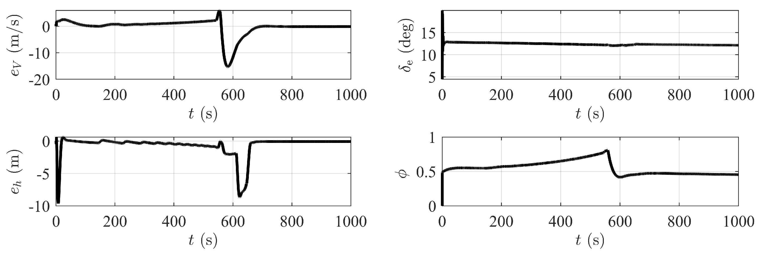
5.2. Tracking Control

The ascent trajectory consists of three phases: constant dynamic ascent, constant Mach ascent, and cruise. The trajectory profile of the mission is designed in Table 3. The initial velocity and altitude are selected as 6.5 and 23,408 m, and the final cruise velocity and altitude are given as 7.8 and 26,759 m.
The tracking errors and control are provided in Figure 6. The velocity and altitude can track the given commands well, and the angle of attack and control inputs can keep within the expected range. These results show the effectiveness of the designed control system, and the relative tracking error is too small to climb the given task point.

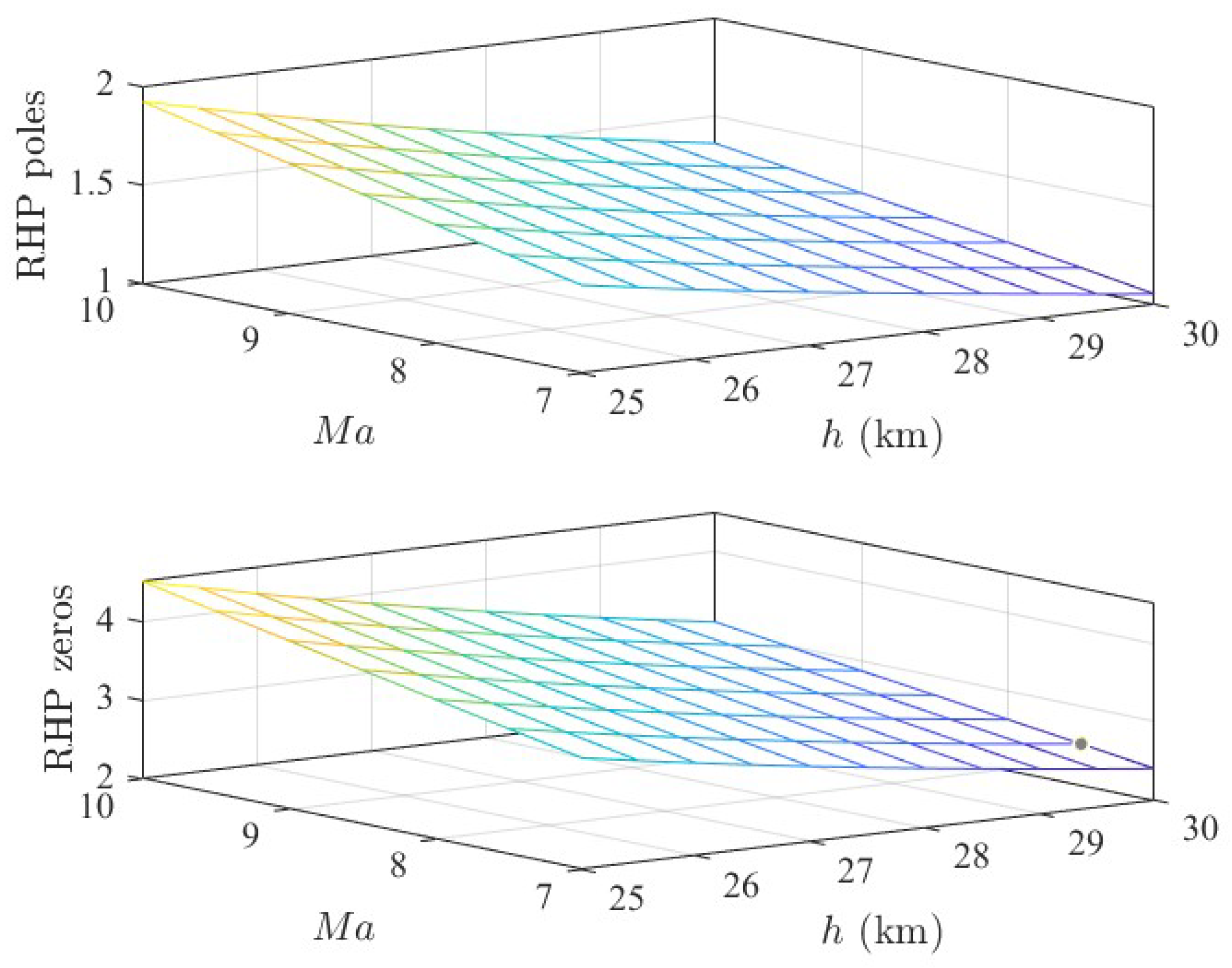
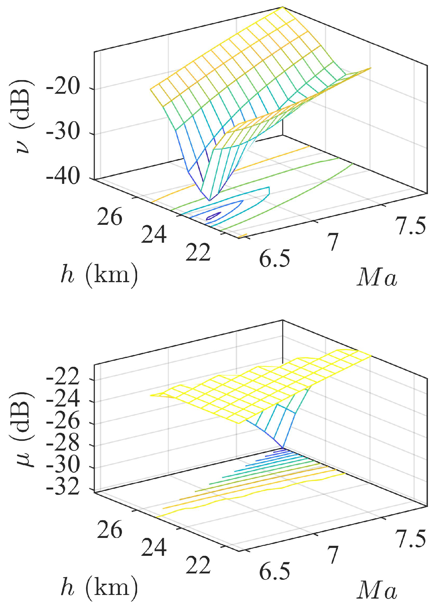
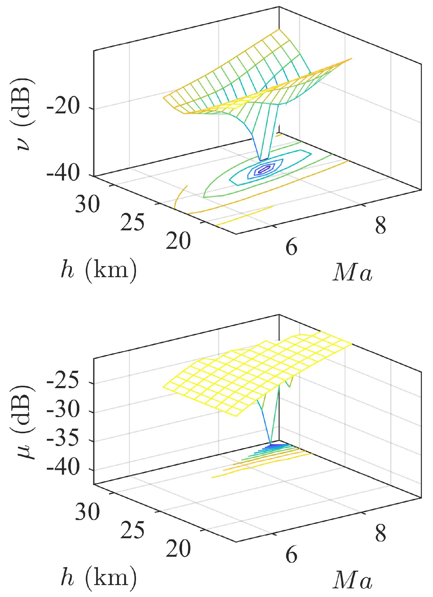
5.3. Robust Analysis

The initial parameters of the tracking controller are obtained at the start point in constant dynamic pressure climb. The gap metric is computed for the open-loop system varying due to flight condition. The normalized coprime stability margin (NCSM) of the closed-loop system is calculated for the same controller obtained at the design point. Here, we provide two examples to illustrate the robust analysis based on gap margin, as shown in Figure 7 and Figure 8.
The value of NCSM and the gap metric are expressed in dB. The tendency of the gap metric shows a significant relation with dynamic pressure. Furthermore, it decreases as the velocity deviates from the design point, revealing the variation in open-loop dynamics with flight conditions. As for closed-loop dynamics, the nominal controller at the initial point is used for all cases in the flight envelope. Hence, the NSCM reveals the robustness of the closed-loop system if we keep the controller the same. The nominal value of NSCM for the start point is approximately 0.1. It dramatically decreases as the flight altitude increases by 2 km, whereas it remains as velocity increases. Moreover, simulation results show the same tendencies for the terminal points compared with the initial point. The evaluated gap margins for these two cases are provided in Figure 9. The circle in these figures represents the initial flight condition of ascent, whereas the square is the terminal point. Besides, the blue line denotes the constant dynamic pressure profile, and the orange line denotes the constant Mach number provile.
A positive gap margin reveals the robustness of the closed-loop system, whereas a negative gap margin indicates that the closed-loop system lacks robust stability. Simulation results reveal that the trajectory tracking control is more sensitive to altitude variation. A deviation of 800 m will cause stability problems, whereas the range of velocity deviation is about 210 m/s. It indicates that climbs with constant velocity for hypersonic vehicles need more attention for precise altitude control.

6. Conclusions

This paper develops a rapid modeling method of an aerospace vehicle and proposes a robust analysis method based on the gap metric. Simulation results validate the proposed model of the aerospace vehicle in terms of longitudinal dynamics. The structure of the polynomial fitting model is proven to be efficient for guidance and flight control. Hypersonic ascent trajectory is optimized by accelration profile using the velocity-driven method. Moreover, a robust analysis method is proposed and validated for ascent tracking control. The difference in hypersonic dynamics tends to be more sensitive to dynamic pressure. Furthermore, the closed-loop robustness regarding the normalized coprime stability margin (NCSM) is closely related to altitude. The gap margin is proposed to qualify the robustness. Simulation results reveal that a deviation of 800 m in altitude will cause stability problems, whereas the range of velocity deviation is about 210 m/s. Hence, the ascent tracking control for hypersonic vehicles needs more attention for precise altitude control.

Author Contributions

Methodology, Y.L. (Yiran Liu); Software, B.C.; Validation, Y.L. (Yanbin Liu); Formal analysis, J.C. All authors have read and agreed to the published version of the manuscript.

Funding

This study was co-supported by the Natural Science Foundation of Jiangsu Province, China (No. BK20200437), the National Natural Science Foundation of China (No. 62103187) and the Fundamental Re-search Funds for the Central Universities, China (No. NT2022025 and No. NS2021061).

Institutional Review Board Statement

Not applicable.

Informed Consent Statement

Not applicable.

Data Availability Statement

Not applicable.

Conflicts of Interest

The authors declare no conflict of interest.

References

  1. Chen, K.; Pei, S.; Shen, F.; Liu, S. Tightly Coupled Integrated Navigation Algorithm for Hypersonic Boost-Glide Vehicles in the LCEF Frame. Aerospace 2021, 8, 124. [Google Scholar] [CrossRef]
  2. Wang, G.Z.; Huang, W.; Yan, L. Multidisciplinary design optimization approach and its application to aerospace engineering. Chin. Sci. Bull. 2014, 59, 5338–5353. [Google Scholar] [CrossRef]
  3. Liu, Y.; Chen, B.; Li, Y.; Shen, H. Overview of control-centric integrated design for hypersonic vehicles. Astrodynamics 2018, 2, 307–324. [Google Scholar] [CrossRef]
  4. Chavez, F.R.; Schmidt, D.K. Analytical Aeropropulsive/Aeroelastic Hypersonic-Vehicle Model with Dynamic Analysis. J. Guid. Control Dyn. 1994, 17, 1308–1319. [Google Scholar] [CrossRef]
  5. Clark, A.; Mirmirani, M.; Choi, S.; Wu, C.; Mathew, K. An Aero-Propulsion Integrated Elastic Model of a Generic Airbreathing Hypersonic Vehicle. In Proceedings of the AIAA Guidance, Navigation, and Control Conference and Exhibit, Keystone, CO, USA, 21–24 August 2006. [Google Scholar]
  6. Bolender, M.A.; Doma, D.B. Nonlinear Longitudinal Dynamical Model of an Air-Breathing Hypersonic Vehicle. J. Spacecr. Rocket. 2007, 44, 374–387. [Google Scholar] [CrossRef]
  7. Oppenheimer, M.W.; Doman, D.B. A Hypersonic Vehicle Model Developed With Piston Theory. In Proceedings of the AIAA Atmospheric Flight Mechanics Conference and Exhibit, Keystone, CO, USA, 21–24 August 2006. [Google Scholar]
  8. Parker, J.T.; Serrani, A.; Yurkovich, S.; Bolender, M.A.; Doman, D.B. Control-Oriented Modeling of an Air-Breathing Hypersonic Vehicle. J. Guid. Control. Dyn. 2007, 30, 856–869. [Google Scholar] [CrossRef]
  9. Frendreis, S.G.; Cesniky, C.E. 3D Simulation of Flexible Hypersonic Vehicles. In Proceedings of the AIAA Atmospheric Flight Mechanics Conference, Toronto, ON, Canada, 2–5 August 2010. [Google Scholar]
  10. Whitmer, C.; Kelkar, A.; Vogel, J.; Chaussee, D.; Ford, C. Control Centric Parametric Trade Studies for Scramjet-Powered Hypersonic Vehicles. In Proceedings of the 2010 AIAA Guidance, Navigation, and Control Conference, Toronto, ON, Canada, 2–5 August 2010. [Google Scholar]
  11. Tsuchiya, T.; Takenaka, Y.; Taguchi, H. Multidisciplinary Design Optimization for Hypersonic Experimental Vehicle. AIAA J. 2007, 45, 1655–1662. [Google Scholar] [CrossRef]
  12. Chen, B.; Liu, Y.; Lei, H.; Shen, H.; Lu, Y. Ascent trajectory tracking for an air-breathing hypersonic vehicle with guardian maps. Int. J. Adv. Robot. Syst. 2017, 14, 1–11. [Google Scholar] [CrossRef]
  13. Chen, B.; Liu, Y.; Shen, H.; Lu, Y. Surrogate modeling of a 3D scramjet-powered hypersonic vehicle based on screening method IFFD. Proc. Inst. Mech. Eng. Part J. Aerosp. Eng. 2017, 231, 265–278. [Google Scholar]
  14. Starkey, R.P.; Rankins, F.; Pines, D. Coupled Waverider/Trajectory Optimization for Hypersonic Cruise. In Proceedings of the 43rd AIAA Aerospace Sciences Meeting and Exhibit, Reno, NV, USA, 10–13 January 2005. [Google Scholar]
  15. Chen, B.; Liu, Y.; Shen, H.; Lei, H.; Lu, Y. Performance limitations in trajectory tracking control for air-breathing hypersonic vehicles. Chin. J. Aeronaut. 2019, 32, 167–175. [Google Scholar] [CrossRef]
  16. Xu, B. Robust adaptive neural control of flexible hypersonic flight vehicle with dead-zone input nonlinearity. Nonlinear Dyn. 2015, 80, 1509–1520. [Google Scholar] [CrossRef]
  17. Qin, W.; He, B.; Liu, G.; Zhao, P. Robust model predictive tracking control of hypersonic vehicles in the presence of actuator constraints and input delays. J. Frankl. Inst. 2016, 353, 4351–4367. [Google Scholar]
  18. Xiao, D.; Liu, M.; Liu, Y.; Lu, Y. Switching control of a hypersonic vehicle based on guardian maps. Acta Astronaut. 2016, 202, 294–306. [Google Scholar] [CrossRef]
  19. Kulfan, B.M. Universal Parametric Geometry Representation Method. J. Aircr. 2007, 45, 142–158. [Google Scholar] [CrossRef]
  20. Skujins, T.; Cesnik, C.E.; Oppenheimer, M.W.; Doman, D.B. Canard-Elevon Interactions on a Hypersonic Vehicle. J. Spacecr. Rocket. 2010, 47, 90–100. [Google Scholar] [CrossRef]
  21. Torrez, S.M.; Driscoll, J.F.; Dalle, D.J. Hypersonic Vehicle Thrust Sensitivity to Angle of Attack and Mach Number. In Proceedings of the AIAA Atmospheric Flight Mechanics Conference, Chicago, IL, USA, 10–13 August 2009. [Google Scholar]
  22. Dalle, D.J.; Torrez, S.M.; Driscoll, J.F.; Bolender, M.A.; Bowcutt, K.G. Minimum-Fuel Ascent of a Hypersonic Vehicle Using Surrogate Optimization. J. Aircr. 2014, 51, 1973–1986. [Google Scholar] [CrossRef]
  23. Dickeson, J.; Rodriguez, A.; Sridharan, S.; Korad, A. Elevator Sizing, Placement, and Control-Relevant Tradeoffs for Hypersonic Vehicles. In Proceedings of the AIAA Guidance, Navigation, and Control Conference, Toronto, ON, Canada, 2–5 August 2010. [Google Scholar]
  24. Kelkar, A.G.; Vogel, J.M.; Inger, G.; Whitmer, C.; Sidlinger, A.; Ford, C. Modeling and Analysis Framework for Early Stage Trade-off Studies for Scramjet-Powered Hypersonic Vehicles. In Proceedings of the 16th AIAA/DLR/DGLR International Space Planes and Hypersonic Systems and Technologies Conference, Norfolk, VA, USA, 19–22 October 2009. [Google Scholar]
  25. Morelli, E.A. Flight-Test Experiment Design for Characterizing Stability and Control of Hypersonic Vehicles. J. Guid. Control. Dyn. 2009, 32, 949–959. [Google Scholar] [CrossRef]
  26. Frendreis, S.G.; Skujins, T.; Cesnik, C.E. Six-Degree-of-Freedom Simulation of Hypersonic Vehicles. In Proceedings of the AIAA Atmospheric Flight Mechanics Conference, Chicago, IL, USA, 10–13 August 2009. [Google Scholar]
  27. Wang, S.X.; Zhang, Y.; Jin, Y.Q.; Zhang, Y.Q. Neural control of hypersonic flight dynamics with actuator fault and constraint. Sci. China Inf. Sci. 2015, 58, 1–10. [Google Scholar] [CrossRef]
  28. Liu, Z.Y.; Li, Z.Y. L1 Adaptive Loss Fault Tolerance Control of Unmanned Hypersonic Aircraft with Elasticity. Aerospace 2021, 8, 176. [Google Scholar] [CrossRef]
  29. Marcos, A.; Balas, G.J. Development of Linear-Parameter-Varying Models for Aircraft. J. Guid. Control Dyn. 2004, 27, 218–228. [Google Scholar] [CrossRef]
Figure 1. Geometrical configuration of aerospace vehicle.
Applsci 13 05189 g001
Figure 2. Comparison diagram for the aerodynamic model.
Applsci 13 05189 g002
Figure 3. Comparison diagram for the propulsive model.
Applsci 13 05189 g003
Figure 4. Research course on the simulation model.
Applsci 13 05189 g004
Figure 5. Poles and zeros of the right half plane.
Applsci 13 05189 g005
Figure 6. Response of trajectory tracking.
Applsci 13 05189 g006
Figure 7. NCSM and gap metric of ascent tracking at Mach 6.5, h = 23,408 m.
Applsci 13 05189 g007
Figure 8. NCSM and gap metric of ascent tracking at Mach 7.8, h = 26,495 m.
Applsci 13 05189 g008
Figure 9. Gap margin of ascent tracking.
Applsci 13 05189 g009
Table 1. The matching function of the polynomial model.
CoefficientsVAFRMSE
C L 99.08%0.0007
C D 98.04%0.00008
C m 98.36%0.0022
C T 90.82%0.0094
Table 2. Trim values of hypersonic vehicles.
MachAltitude (km)AOA (deg)Elevon Deflection Angle (deg)FER
6252.164514.44880.391
7261.907313.65130.4044
8271.725313.12180.4393
9281.601612.76700.4811
10291.522412.53510.5309
Table 3. Initial points of the different phases.
Phases h 0 ( m ) V 0 ( m ) Ma 0 Ma 1
Constant dynamic pressure23,40825,7696.57.8
Constant Mach number25,76926,4957.87.8
Cruise flight26,49526,4957.87.8
Disclaimer/Publisher’s Note: The statements, opinions and data contained in all publications are solely those of the individual author(s) and contributor(s) and not of MDPI and/or the editor(s). MDPI and/or the editor(s) disclaim responsibility for any injury to people or property resulting from any ideas, methods, instructions or products referred to in the content.

