Convolved Feature Vector Based Adaptive Fuzzy Filter for Image De-Noising

Featured Application

The proposed mechanism can be used as pre-processing module in any image processing related application.

Abstract

In this paper, a convolved feature vector based adaptive fuzzy filter is proposed for impulse noise removal. The proposed filter follows traditional approach, i.e., detection of noisy pixels based on certain criteria followed by filtering process. In the first step, proposed noise detection mechanism initially selects a small layer of input image pixels, convolves it with a set of weighted kernels to form a convolved feature vector layer. This layer of features is then passed to fuzzy inference system, where fuzzy membership degrees and reduced set of fuzzy rules play an important part to classify the pixel as noise-free, edge or noisy. Noise-free pixels in the filtering phase remain unaffected causing maximum detail preservation whereas noisy pixels are restored using fuzzy filter. This process is carried out traditionally starting from top left corner of the noisy image to the bottom right corner with a stride rate of one for small input layer and a stride rate of two during convolution. Convolved feature vector is very helpful in finding the edge information and hidden patterns in the input image that are affected by noise. The performance of the proposed study is tested on large data set using standard performance measures and the proposed technique outperforms many existing state of the art techniques with excellent detail preservation and effective noise removal capabilities.

1. Introduction

Image de-noising is a challenging pre-processing step in the domain of digital image processing (DIP) and computer vision (CV). The main goal of image de-noising is to reinstate the noisy pixel as close as possible to the original pixel using image de-noising techniques. Noise is an uncertain phenomenon which may introduce in an image by faulty sensors during image acquisition, storage or transmission, etc. Furthermore, when we quantize on an image, we may lose some important details of that image [1]. If the image contains noise, then succeeding image processing processes such as object detection, image segmentation and tracking etc., may perform poorly on the input image [2]. Therefore, image de-noising is a vital part and may require additional pre-processing steps in all the domains that uses images as input.

A number of linear and non-linear image de-noising techniques have been proposed during the last few decades. Linear techniques replace noisy pixels by average value of the kernel causing blurry effects on the edges due to the removal of crisp information. On the other hand, non-linear techniques [3,4,5,6,7,8,9,10] are preferred over linear techniques [11,12,13] because of their non-linear nature and robustness against noise. These techniques do not interrupt the image details to great extent causing better restored results. In this review section, we will focus mainly on non-linear techniques. The main filter in non-linear techniques is median filter, easy in implementation, and is used as most common tool in many other techniques. It gives best performance for images having smooth variations and low level of impulse noise but gives inadequate performance for highly contrast detailed images corrupted with high noise densities because its mechanism simply use median to replace the central corrupted pixel in both the cases. Furthermore, edges [14] are most important parts of the image and they are directly affected by the size of the kernel. So design of the kernel in non-linear filters is equally important to avoid blurring effects at edges. Kernel with a small size (say 3 × 3) is very effective for low noise densities or where the total number of corrupted pixels are fewer than half of the size of kernel. Kernel sizes greater than previously described size might smear lines and edges in detailed regions of the image due to indiscriminate gray level substitutions.

In last few decades, a large number of variations [4,5,6,7,8,9,10,15,16,17,18] have been proposed in median filter to enhance its computational power, detail preservation and noise suppression capabilities. Median filters based techniques [4,5,6,7,8,9,10] simply replace the degraded pixel value by median of neighborhood pixels whereas weighted median techniques [5,6,8,16] use weighing mechanism for good and bad ones. All of the above filters are efficient against impulse noise but fail due to blurring [11,12,13] at edges and loss of actual details in an image. Switching mechanisms [9,17], fuzzy based techniques [19,20,21,22,23,24,25,26,27,28], directional filters [15,16,22,24] and others [29,30,31,32,33,34,35,36,37,38,39] are good de-noising filters against random and universal noise but still lacking in detail preservation due to poor or no proper edge detection.

Fuzzy logic has added excellent noise removal capabilities against different types of noise due to uncertainty features [19,20,21,22,23,24,25,26,27,28,32]. A fuzzy logic based filtering mechanism is proposed in [19] for additive noise, which is mainly, based on fuzzy image derivatives in eight directions. This fuzzy filter gives good results but edges and sharp details of the image are not well preserved. Schulte et al. in [20] proposed a fuzzy logic based nonlinear filtering mechanism to address the problem in above said filter. Kang et al. in [22] proposed a directional mechanism in four directions based on fuzzy reasoning. The main drawback was in non-adaptive behavior of the threshold parameters. Toh et al. in [23] proposed cluster-based approach for better classification of impulse noise but was unsuccessful at low and very high noise densities. Hussain et al. in [24,25] proposed fuzzy reasoning based clustering criteria of pixels to address the problems in above filters. Similar fuzzy logic based other filters [26,27,28,32] address neighboring issues and hybrid approaches for effective impulse noise removal.

In this paper, a new fuzzy inference system based impulse noise removal technique is proposed that uses a convolved feature vector layer to effectively restore the corrupted image details. The proposed technique first extracts a small layer of pixels from input image, convolves it to form a convolved feature vector layer and forward this layer to fuzzy inference system to determine the noise type in that particular patch. Fuzzy membership degrees play a vital role in filtering phase to remove the corrupted pixels. Noise-free pixels remain unaffected throughout this process contributing maximum detail preservation.

The paper is organized as follows: Noise model and reviews are presented in Section 2 and Section 3, respectively. Methodology of the proposed filter is described in Section 4. Experimental setup, results and discussions are briefly explained in Section 5 whereas conclusions are drawn in Section 6.

2. Noise Model

In this paper, we mainly focused on impulse noise [1] which can be categorized into two types, fixed value impulse noise (FVIN) and random value impulse noise (RVIN). In FVIN, corrupted image pixels are replaced with either 0 or 255 whereas in RVIN corrupted pixels can be replaced by any grayscale value from [0–255]. It is clear from the above description that removal of RVIN is more challenging than FVIN. Let N_i,j and x_i,j represent noisy and noise-free pixel values at (i,j) then impulse noise model for RVIN can be described as follows:

$$N_{i,j}=\{\begin{array}{ll}{g}_{i,j},& \mathrm{with}\mathrm{probability}\eta \\ x_{i,j},& \mathrm{with}\mathrm{probability}1-\eta \end{array}$$

(1)

where g_i,j represents gray level value of corrupted pixel. The main sources of noise include all those processes involved in acquisition, storage and transmission of the digital image.

3. Basic Reviews

In this part, we first review a couple of basic components that are widely used in development of impulse noise removal filters.

3.1. Median Filter

In Section 1 (literature review), we have seen that median filter and its different variants are still very effective and widely used for impulse noise removal as well as image detail preservation. The mechanism of median filter is very simple, returns the central value of any processing window/kernel after sorting in ascending or descending order. A simple median filter can be modeled as,

$$M=Median\{a_1,a_2,\dots ,a_n\}$$

(2)

where a_n represent ordered list elements of the processing window/kernel.

3.2. Deviation from a Reference Point

Simple median filter and its variations are quite effective for the images having smooth regions/variations or when the noise ratio in an image is very low. For all other cases, the performance is badly affected due to non-utilization of neighboring pixels. To address this problem, the second most important component used in filter design is absolute deviation of each element/pixel from a certain reference point. This reference point can be any constant number, median type variable or a statistical parameter which can be modeled as,

$$AD(p_{i,j})=|p_{i,j}-r|,p_{i,j}\in \mathsf{\Omega }$$

(3)

where r is a reference point, p_i,j represents each element of Ω which is a kernel in this case. The subsequent values are then further checked with a certain value called ‘threshold’ to construct a noise map (NM) as,

$$NM=\{\begin{array}{l}1,\hspace{1em}AD(p_{i,j})\ge threshold\\ 0,\hspace{1em}Otherwise\end{array}$$

(4)

where ‘threshold’ can be fixed or adaptive.

The techniques explained above are essential part of most of the impulse noise removal filters. Fuzzy logic based pixel density based models [19,20], reasoning model [22], switching [23], directional [24], clustering model [25], computation models [27] and hybrid filter [28] use generic linear and non-linear statistical methods which may produce good results under certain conditions due to non-linear nature of the median filter but generality is not true. Cluster based median filter (CMF) [25], region adaptive filter (RAF) [26], new weighted mean (NWM) filter [29] and others [5,6,7,8,9,10,11,12,13,14,15,16,17,18,19,20,30,31,32,33,34] mainly use above said criteria’s in noise detection phases. CMF works well against salt & peppers noise but gives unsatisfactory results against random noise. CMF, RAF and NWM use fixed threshold values (threshold = 12 to threshold = 22) during noise detection process which may give satisfactory performance for certain type of images but may lead to wrong classification of noisy and noise free pixels for large datasets against random noise.

3.3. Why Convolved Feature Vector (CFV)?

Most of the impulse noise removal techniques explained and reviewed in previous sections use specific computational mechanisms to estimate the central pixel value of the kernel to be noisy or noise-free. These mechanisms may produce good results under certain conditions but generality is not true in all cases. For example, median filter outperforms many filters if the input image is smooth and have low noise densities, i.e., when the number of degraded pixels are fewer than half of the size of kernel. In all other cases, median filter may replace incorrect pixel values causing blurry effects. This idea is explained in Figure 1 where a standard ‘Barbara’ image is artificially degraded with three types of impulses. In Figure 1a, a smooth region is artificially degraded with RVIN, whereas Figure 1b,c are degraded with high noise ratio of salt and peppers like impulses. In Figure 1b,c central pixels are identified as noise-free when a simple median filter defined in (2) is used to detect or remove the additive noise. Furthermore, absolute differences or deviations from their medians and central pixels are zero, which indicates strong relationship among the majority of neighboring pixels. In Figure 1c, two kernels are considered where the upper kernel is degraded artificially with random noise and lower kernel is noise-free. Median values of upper and the lower kernels are 171 and 169, respectively. Likewise, absolute differences are 9 and 10, respectively. These features establish a fact that both the kernels contain almost are similar features whereas one kernel is noise-free and the other one is noisy. Similar noise detection and removal problems ascend in [35,36,37] due to ineffective use of median filter and thresholds. In most cases, when features are alike, noise detection and removal becomes problematic. Furthermore, when noise ratio becomes high in small size kernels (as in Figure 1a,b), similar problem arises. To overcome this problem, we have proposed a new convolved feature vector based fuzzy mechanism in this paper.

4. Proposed Methodology: Convolved Feature Vector Based Fuzzy Filter

Generally, in noise removal techniques, two key conventions are considered. Firstly, the image that is noise-free usually comprises of smooth regions separated by edges and lines. Secondly, smooth regions, edges and lines in a noisy image do not disclose compatibility with neighboring pixels and intensity transformations are also very abrupt. Furthermore, kernel size is very important for feature extraction and analysis. Small size kernel i.e., 3 × 3 is considered very effective in terms of computation but gives inadequate performance at high noise. Also, the edge and texture information is limited in small size kernel. Large size kernels, i.e., 5 × 5 and above adds more textures and edges information around a certain pixel but they are cost effective in terms of computation. Furthermore, median drifting problems usually occur in large size kernels causing blurry effects on restored images.

Keeping in view the above assumptions and limitations, a convolved feature vector (CFV) based fuzzy mechanism is introduced which consists of two steps, noise detection followed by noise filtering. In noise detection phase, noisy pixels are judged based on its neighboring pixels as well as fuzzy rules-based mechanism. Pixel having traces of noise are filtered out in filtering phase based on fuzzy membership degrees.

4.1. Noise Detection Mechanism

Our noise detection mechanism plays a vital role to isolate the noisy pixels and is mainly comprises of two steps: ‘divide and conquer strategy’ and fuzzy based contextual model.

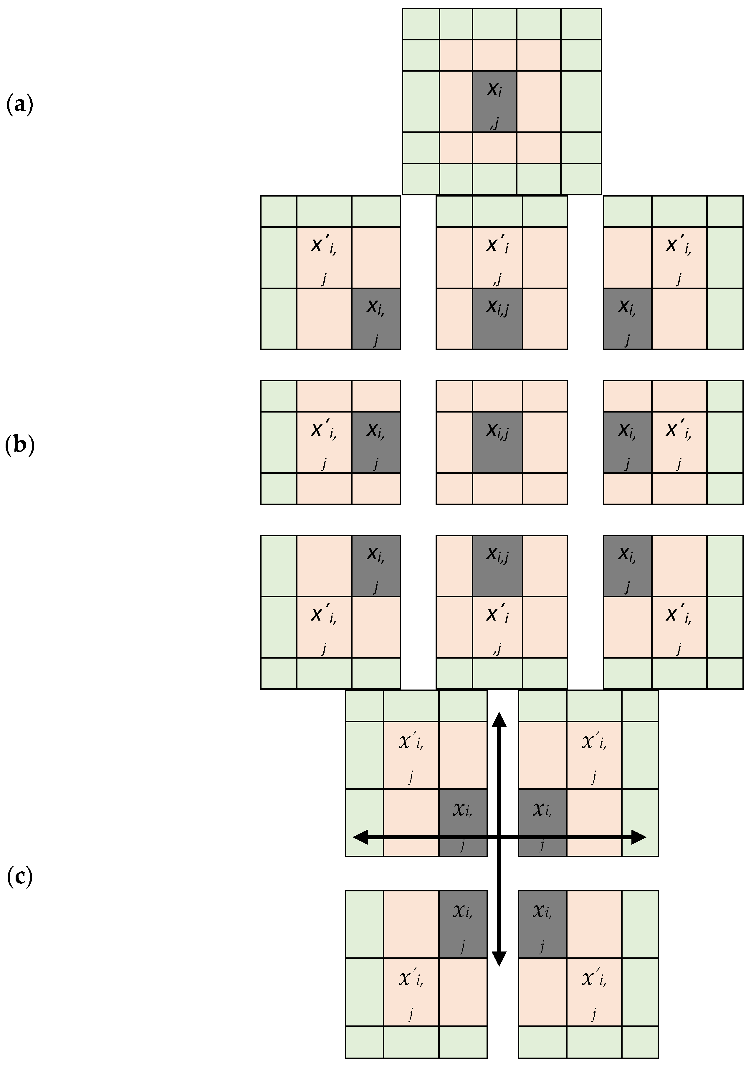
4.1.1. Divide and Conquer Strategy

Existing noise removal techniques use a typical style of noise detection, i.e., central pixel is judged based on its neighboring pixels and some threshold. We have introduced a new mechanism in which the central location of each kernel is changed all together by adding more neighbors to existing kernel and dividing the new (large) kernel to produce more kernels of the same size of original kernel. For example, if we have a 3 × 3 kernel then by adding one neighbor along its each side will produce a 5 × 5 kernel with the same center as shown in Figure 2a. Now, by diving 5 × 5 kernel to the same size as of the original kernel will produce 9 subsets of size 3 × 3 as shown in Figure 2b. It can be seen from the Figure 2b that the position of central pixel has changed and is no more at central location in eight kernels except one kernel lying at center. This strategy can be further extended to 7 × 7, 9 × 9 and 11 × 11 based on noise ratio and noise type but we have restricted our algorithm to just 5 × 5 to avoid computational complexity. Furthermore, in noise detection mechanism, the most critical task is to differentiate the noisy and edge pixels as they possess similar attributes. This division strategy will provide us an extra check to evaluate the noisy and edge pixel lying at central location. Kernels with no or less traces of noise are best candidates for noise estimation.

4.1.2. Fuzzy Based Contextual Model

Nadeem et al. in [38] used nine overlapping sub-windows as shown in Figure 3 for basic processing of noise estimation. In case of low and medium noise, median values of majority of the sub-windows remain unchanged and do not contribute enough in noise estimation process except the limited number. In case of high noise, the probability of lack of texture problem increases in most of the sub-windows. So, the use of all the nine sub-windows increases the computational cost as well as reduces the noise detection capability of the noise detector. The lack of texture problem usually arises when the number of noisy pixels are in large number than half of the size of the kernel and the median value which is now a noisy one replaces the central pixel value of the kernel, resulting in poor detail preservation.

The problem described above can be addressed by selecting limited number of sub-windows/kernels which ultimately help the noise detector for better decision making at noise detection level. In this paper, we have used a simple mechanism for kernel selection, i.e., kernels lying at corners as shown in Figure 2b are selected as potential candidates as these kernels have large number of non-overlapping pixels. The selected kernels reduce the computational cost as well as the lack of texture problem at high noise. These kernels act like quadrants of a Cartesian plane as shown in Figure 2c. Let $W=\left\{x_{i-2,j-2},\dots , x_{i+2,j+2}\right\}$ be a kernel of size 5 × 5 centered at (i,j) containing twenty five (25) pixel locations. After division and kernel selection, let $Q_k^W, k=1, 2, 3, 4,$ be the four subsets of W with new central location at $x_{i,j}^{\prime }$. The pixel locations in four subsets/quadrants are as follows,

$$Q_1^W=\left\{x_{i+l,j+m}:0\le l\le 2,0\le m\le 2\right\}$$

$$Q_2^W=\left\{x_{i+l,j+m}:-2\le l\le 0,0\le m\le 2\right\}$$

$$Q_3^W=\left\{x_{i+l,j+m}:-2\le l\le 0,-2\le m\le 0\right\}$$

$$Q_4^W=\left\{x_{i+l,j+m}:0\le l\le 2,-2\le m\le 0\right\}$$

Median filter defined in Equation (2) can be used to extract the features from the above four quadrants centered at new locations $x_{i,j}^{\prime }$ as fellows,

$$M_k=MED\left\{Q_k^W\right\},k=1,2,3,4,$$

(5)

where M_k is a feature set of pixel locations in four quadrants namely top right, top left, bottom left and bottom right kernels, respectively. Sort the feature set values $M_k, k=1,2,3,4,$ in descending order as $m_1\le m_2\le m_3\le m_4$, where $m_1$ and $m_4$ are the lowest and highest feature values, respectively.

$$\overrightarrow{V}=(m_k),k=1,2,3,4.$$

(6)

$$D^1={\displaystyle \sum _2^4{(\mathrm{m}}_i-m_{i-1})}$$

(7)

$D^1$ is the rank order difference [19] of vector $\overrightarrow{V}$ given in (6). An edge pixel can be separated from noisy pixel if its directional rank-ordered absolute difference (DROAD) [25] in any direction is minimum. For example, after division strategy when the central location of small kernel (subset of large kernel) shifts from $x_{i,j}$ to a new central location $x_{i,j}^{\prime }$ the new and the previous location lie in a certain direction, which should be minimum in case of edge pixel. DROAD values $d_k, k=1,2,3,4,$ in four direction can be calculated as,

$$d_k=\left|{x^{\prime }}_{i,j}-x_{i,j}\right|,k\in Di{r}_k$$

(8)

$$D^2=Min(d_k),k=1,2,3,4.$$

(9)

$D^2$ gives a measure of deviation of central pixel in a certain direction. Large values of $D^1$ and $D^2$ indicate that the pixel under consideration is more likely to be a noisy pixel and vice versa. Any crisp decision at this stage may lead to false prediction and ultimately degradation of the restored image. To avoid this, fuzzy membership degrees can be used to approximate the noise added to the pixels.

We have utilized two fuzzy membership functions Small and Large [22] as shown in Figure 3 and simplified rule base for two inputs of contextual model. Let $Rul{e}_1, n=1,2,3,$ be reduced set of rule numbers defined as,

$${Rule}_1=\mathrm{Small}(D^1,{\lambda }_1,{\lambda }_2)·\mathrm{Small}(D^2,{\lambda }_1,{\lambda }_2)$$

$${Rule}_2=\mathrm{Small}(D^1,{\lambda }_1,{\lambda }_2)\cdot \mathrm{Large}(D^2,{\lambda }_1,{\lambda }_2)|\mathrm{Large}(D^1,{\lambda }_1,{\lambda }_2)\cdot \mathrm{Small}(D^2,{\lambda }_1,{\lambda }_2)$$

$${Rule}_3=\mathrm{Large}(D^1,{\lambda }_1,{\lambda }_2)\cdot \mathrm{Large}(D^2,{\lambda }_1,{\lambda }_2)$$

The two fuzzy membership functions Small and Large are as follows,

$$\mathrm{Small}(D^{\ast },{\lambda }_1,{\lambda }_2)=\{\begin{array}{cc}\hfill 1,\hfill & D^{\ast }<{\lambda }_1\hfill \\ \hfill \left(\frac{D^{\ast }-{\lambda }_2}{{\lambda }_1-{\lambda }_2}\right),\hfill & {\lambda }_1\le D^{\ast }<{\lambda }_2\hfill \\ \hfill 0,\hfill & D^{\ast }\ge {\lambda }_2\hfill \end{array}$$

(10)

$$\mathrm{Large}(D^{\ast },{\lambda }_1,{\lambda }_2)=\{\begin{array}{cc}\hfill 0,\hfill & D^{\ast }<{\lambda }_1\hfill \\ \hfill \left(\frac{D^{\ast }-{\lambda }_1}{{\lambda }_2-{\lambda }_1}\right),\hfill & {\lambda }_1\le D^{\ast }<{\lambda }_2\hfill \\ \hfill 1,\hfill & D^{\ast }\ge {\lambda }_2\hfill \end{array}$$

(11)

where ${\lambda }_1$ and ${\lambda }_2$ are threshold parameters which are set adaptively based on neighboring pixels and are discussed in upcoming section. Fuzzy membership degrees ${\mu }_{Degree}$ for simplified set of rules is calculated as,

$${\mu }_{Degree}=Max[Rul{e}_1,Rul{e}_2,Rul{e}_3]$$

(12)

4.1.3. Adaptive Threshold

A number of existing methods [7,8,9,23,26] for impulse noise removal need either ad-hoc or pre-defined threshold values or settings. There is normally a tradeoff between simple and complex methods, simple methods are good but they may perform poorly under certain conditions whereas complex methods are not always a good choice but they perform better with an extra overhead of computational cost. Furthermore, complex methods sometime require unlike trainings for optimal arrangement of pixels which results in unpredictable responses due to unfitting procedures. Let’s consider an example in which a method is trained on data set containing fairly smooth images having small amount of impulse noise, then its output will surely be a smooth image irrespective of edges and fine details. Similarly, it may perform poorly for a smooth image if it is trained on a data set containing mostly the edges, lines and the fine image details. So the performance may be irregular for the methods that require trainings as they are normally designed for large outlier values and they may fail in prediction when the impulse noise causes a slight variation in the original pixel values.

In response, we have used an adaptive method which neither require training nor the user defined threshold values for noise estimation as well as noise removal. Consider an input image I and a sliding window ${\Omega }^2=\left\{x_{i-2,j-2},\dots , x_{i+2,j+2}\right\}$ of size 5 × 5 placed at center $x_{i,j}$. First of all, we calculate absolute gray-level variances between central pixel and its neighbors aligning in four directions as,

$$A_d(i,j)=\frac{1}{4}\left[{\displaystyle \sum _{p{\mathsf{\epsilon }\mathrm{Dir}}^k}|p-x_{i,j}|}\right]$$

(13)

where $Di{r}^k, k=1, 2, 3, 4,$ denote edge directions in horizontal, vertical and two diagonal directions as shown in Figure 3. Edge and the corrupted pixels usually contribute large A_d(i,j) values which makes the problem more critical. A crisp decision at this stage may lead to false detection as well as poor de-noising results. To avoid this situation, a fuzzy based mechanism is required. We have introduced two parameters α(i,j) and β(i,j) that are used to establish a relationship between edge and a noisy pixel and are calculated as,

$$\alpha (i,j)={\displaystyle \sum _{u=-2}^2{\displaystyle \sum _{v=-2}^2\frac{A_d(i+u,j+v)}{\left|Di{r}^k\right|+9}}}$$

(14)

$$\beta (i,j)=A_d(i,j)$$

(15)

where ${Dir}^k$ denotes total number of directional edge pixels. Consider a pixel lying at central location x_i,j of the sliding window, following fuzzy rule is used to decide whether a pixel under consideration is noisy, edge or noise free pixel.

Fuzzy Rule:

If |α − β| is Large, Then xi,j is a corrupted pixel. Else-If α and β both are Large, Then xi,j is an edge pixel. Else-If α = β, Then xi,j is a noise-free.

As discussed earlier, Large is a fuzzy set [21] and can be represented with a fuzzy membership function as shown in Figure 4. Fuzzy membership degrees which play important role are extracted from a fuzzy membership function Large as follows,

$${\mu }_D(i,j)={\mu }_{\mathrm{Large}}[|\alpha (i,j)-\beta (i,j)|,{\lambda }_1,{\lambda }_2]$$

(16)

In filtering phase, pixels are classified as corrupted or noise-free based on fuzzy membership degrees which are mapped from 0 to 1. Consider a simple example where endpoints of the interval are passed as input to Large, then zero (0) will return a noise-free pixel and one (1) will return a noisy pixel. For all the remaining options between the endpoints, the output remains ambiguous. To solve this problem, we have used another pair of parameters to draw boundary lines between noise free and noisy pixels which can be defined as follows:

$${\lambda }_1(i,j)=\underset{p,q\in \{-2,\dots ,2\}}{Min}[A_d(i+p,j+q)]$$

(17)

$${\lambda }_2(i,j)={\lambda }_1+0.2({\lambda }_1)$$

(18)

If a pixel’s membership degree lies below ${\lambda }_1$ then it’s a noise-free pixel and if its membership value goes beyond ${\lambda }_2$ then it’s a noisy pixel. For all other pixel values that lie in the interval [${\lambda }_1$,${\lambda }_2$] have some percentage of noise which can be easily calculated.

4.2. Noise Detection Mechanism

In filtering phase, fuzzy membership degrees and fuzzy rules play a vital role to classify noise-free, edge and noisy pixels. A pixel having no traces of noise will have membership degrees that lie in Small region. For example, if a pixel whose membership degree is equal to Rule₁, then it’s an edge or noise-free pixel. For all other possibilities, there is a chance of noise present in that pixel values. To remove noise at that locations, a fuzzy based median filter is used which is defined below:

$$\begin{array}{l}\mathit{Filtering} \mathit{Rule}{\displaystyle :}\hspace{1em}\mathit{If} ({\mu }_D=={\mathit{Rule}}_1)\\ \hspace{1em}\hspace{1em} \hspace{1em}\hspace{1em}\hspace{1em}\hspace{1em}\hspace{1em}\hspace{1em}\hspace{1em}\hspace{1em}\hspace{1em}\hspace{1em}\hspace{1em}{y}_{i,i}=x_{i,i}\\ \hspace{1em}\hspace{1em}\hspace{1em}\hspace{1em}\hspace{1em}\hspace{1em}\hspace{1em}\hspace{1em}\hspace{1em}\mathit{Else}\\ \hspace{1em}\hspace{1em}\hspace{1em}\hspace{1em}\hspace{1em}\hspace{1em}\hspace{1em}\hspace{1em}\hspace{1em}\hspace{1em}\hspace{1em}\hspace{1em}\hspace{1em}\hspace{1em}\hspace{1em}{y}_{i,j}={\mu }_D(i,j).Median({\mathsf{\Omega }}^2)+[1-{\mu }_D(i,j)].x_{i,j}\end{array}$$

(19)

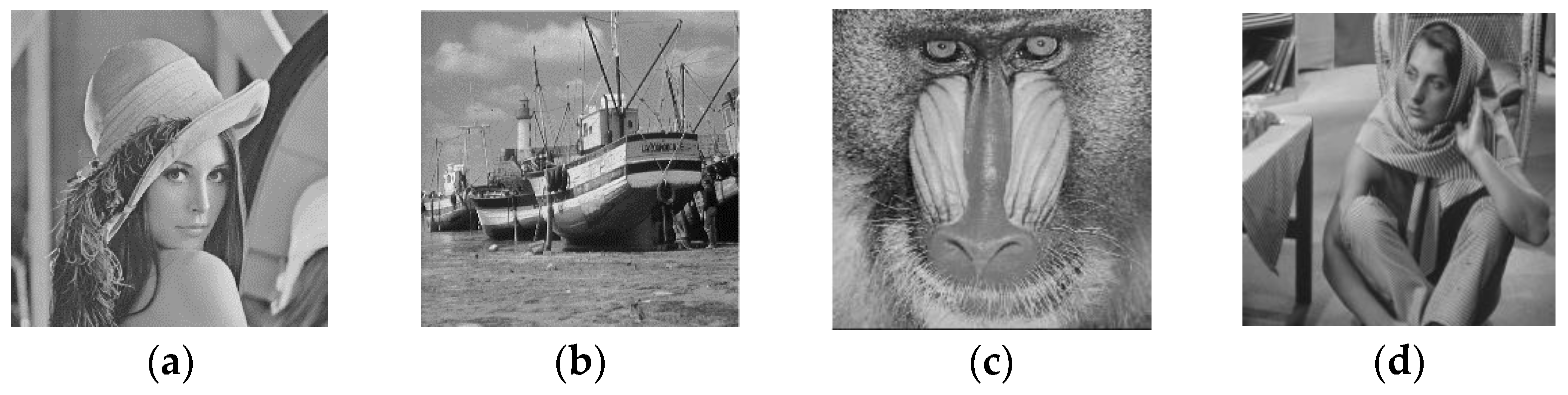
5. Results and Discussions

In this section, a comparison is drawn objectively (numerical results) and subjectively to evaluate the performance of proposed filter with different state of the art noise removal algorithms. The performance of the proposed filter is analyzed based on a large data set of images including medical images dataset MedPix obtainable at http://www.imageprocessingplace.com (accessed on 1 July 2022). The evaluation is not restricted to 512 × 512 only but of different sizes. Image are first degraded with impulse noise defined in (1) with different noise ratios starting from 10% and above and then proposed algorithm is tested. MATLAB R2021a is used for implementation of proposed model. All the experiments are performed on Intel Core i7 processor with 2.11 GHz clock speed and 16 GB of RAM.

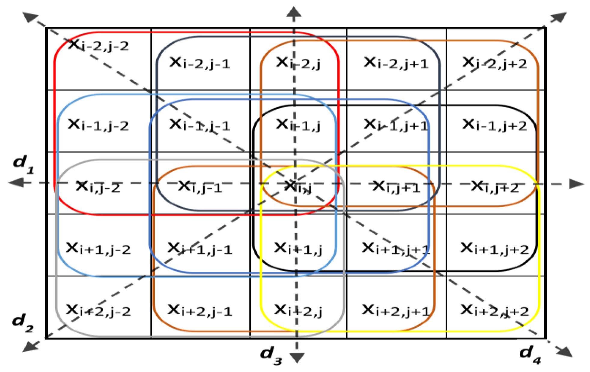
5.1. Settings: Processing Windows/Kernels

As discussed in previous section, the proposed algorithm is based on divide and conquer mechanism which divides as large size processing window into small size sub-windows for effective noise estimation. Any processing window larger than 3 × 3 can be used for implementation purposes. We have tested our technique on different processing windows of sizes 5 × 5, 7 × 7, 9 × 9 and 11 × 11 and have found that larger is the size of processing window greater is the blurry effects at edges and borders. The processing window of size 5 × 5 gives best results in terms of PSNR and visual quality. So, in this paper, we have chosen a processing window of size 5 × 5 as our initial basic window size as it gives optimum results at different noise densities ranging from low to high. Another parameter that is equally important is the number of iterations at which the proposed technique gives best PSNR values. Figure 5 shows ten (10) times filtered results in terms of PSNR of four images corrupted with noise ratio of 50%. The PSNR value of each image at first iteration is less than the upcoming iterations because some corrupted pixels are not detected and not filtered out. It is also clear from Figure 5 that that proposed filter achieves its optimum PSNR values at 4th iteration and remains unchanged at subsequent iterations just because most of the corrupted pixels have been detected and filtered out in previous iterations.

5.2. Performance of the Proposed Noise Detector

In gray-scale images, the performance of noise detector badly affects when noise brings slight or abrupt changes to image pixel values as slight changes are sometimes ignored whereas abrupt change is an indication of an edge. So, there is a strong possibility that noisy and clean pixels are miss or falsely classified by the noise detector. A good noise detector with less number of miss detection (MD) and false detection (FD) cases can lead to better restoration results.

Table 1. Detection results comparison of different methods for Lena image when corrupted with 30% to 60% RVIN.

Ratio Methods		30%			40%			50%			60%
	MD	FD	Total	MD	FD	Total	MD	FD	Total	MD	FD	Total
DWM [16]	9081	6550	15631	9499	7771	17,270	9511	11,380	20,891	12,701	12,298	24,999
NWM [29]	9578	6012	15,590	10,150	6220	16,370	11,126	8303	20,429	15,450	7551	23,001
ACWM [8]	14,340	2023	16,363	16,048	2164	18,212	23,690	3641	27,331	32,733	7702	40,435
SDOOD [39]	10,508	9672	20,180	12,273	10,325	22,598	13,745	15,599	27,344	14,952	12,833	27,785
SRM [40]	15,894	1998	17,892	21,076	2571	23,647	24,922	4204	29,126	32,719	6550	39,269
AEPWM [41]	9940	8028	17,968	10,910	7975	18,885	11,675	9617	21,292	13,571	9769	23,340
AFIDM [42]	7112	6334	13,446	8209	7069	15,278	8508	8375	15,483	8978	8894	17,872
QSAF [38]	5122	5899	11,021	5509	6311	11,820	6919	8025	14,944	9055	9240	18,295
TSA [35]	9890	5002	14,892	11,039	4215	15,254	13563	5284	18,847	15,070	7522	22,592
Proposed	5233	4865	10,098	5324	6208	11,532	7513	6828	14,341	9991	7428	17,419

shows a quantitative comparison of different noise detectors for Lena image corrupted with different noise ratios ranging from 30% to 60% random valued impulse noise (RVIN). QSAF at 30% RVIN has least number of MD pixels but large number of FD pixels whereas SRM has very low FD and high MD rate. Similarly, our proposed filter at 40% RVIN has a low MD rate but high FD rate whereas ACWM has very low FD rate and a very high MD rate. Furthermore, it can be seen from the Table 1 that total number of MD and FD pixels of our proposed filter has least number as compared to other noise detectors at different noise level.

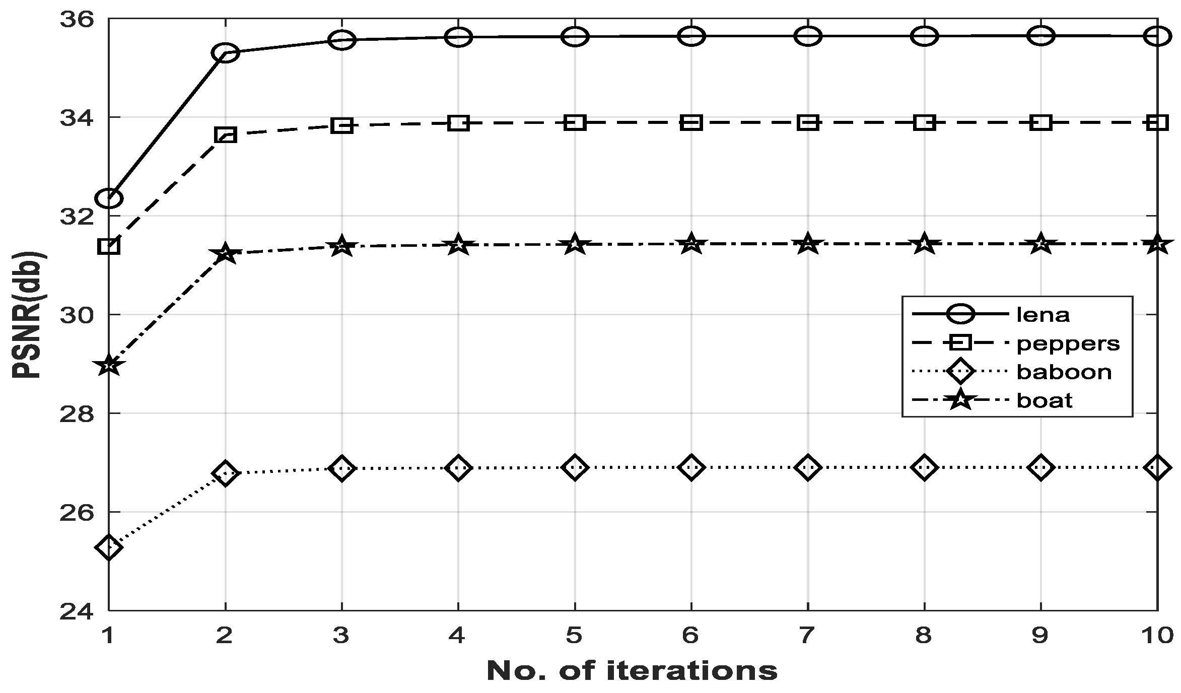
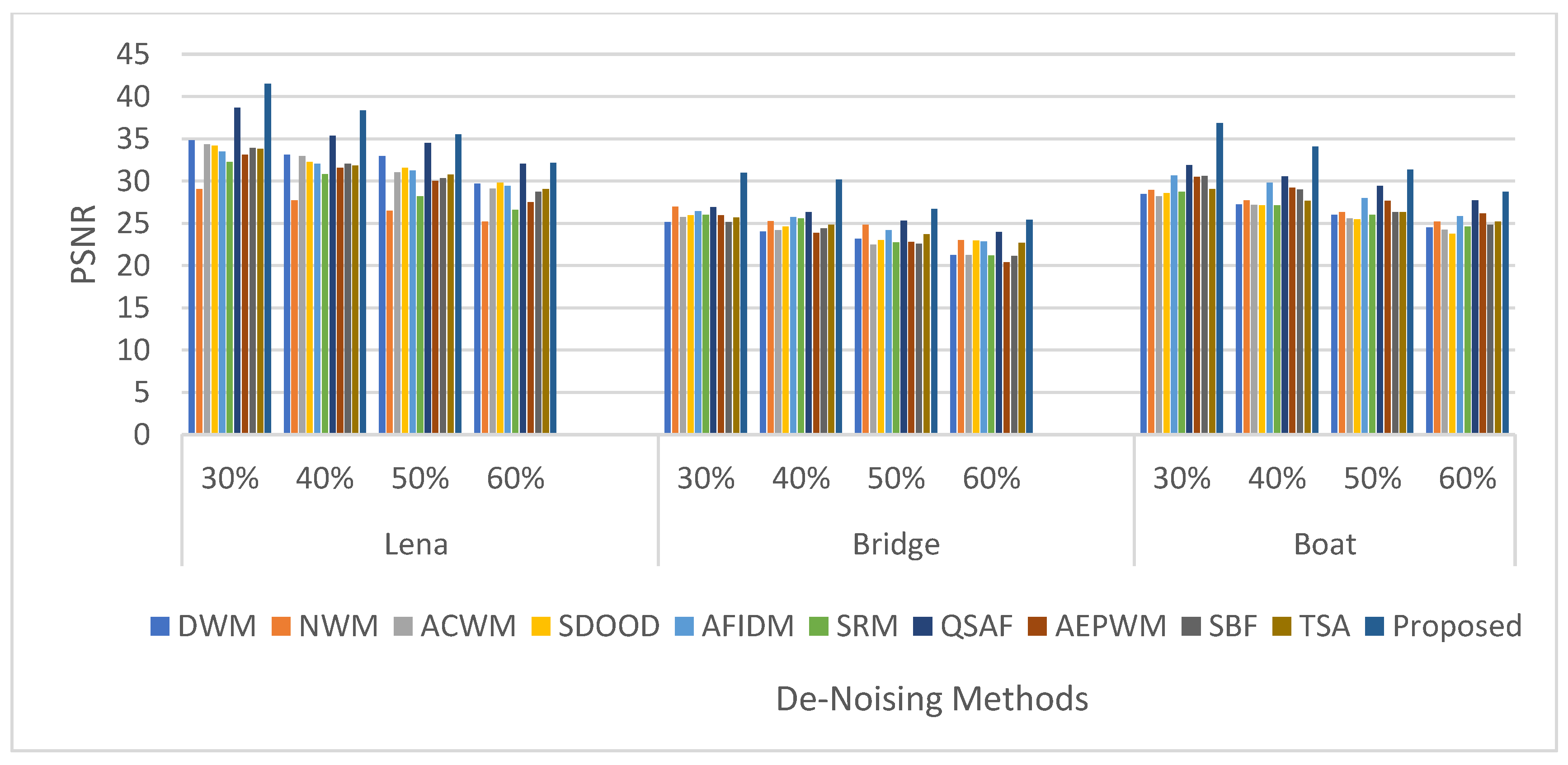
5.3. Performance of the Proposed De-Noising Filter

In this section, another quantitative analysis of de-noised images is performed to evaluate the performance of our proposed filter with other de-noising filters. Three performance measures, peak signal to noise ratio (PSNR), structure similarity index measure (SSIM) and edge preservation index (EPI) [33] are used on standard test images as shown in Figure 6 for basic quantitative comparisons. Figure 7 shows PSNR values for Lena, Bridge and Boat image against different noise densities of RVIN ranging from 30% to 60%. It is clear from the bar chart that that proposed de-noising filter gives excellent results in terms of PSNR against all the competing filters and outperforms them against different noise levels of RVIN with a good margin.

Table 2. Comparison of results in terms of SSIM for Lena, Bridge and Boat images corrupted with 30% to 60% RVIN.

Methods	DWM	NWM	ACWM	SDOOD	AFIDM	SRM	QSAF	AEPWM	SBF	TSA	Proposed
Lena
30%	0.914	0.831	0.936	0.920	0.938	0.918	0.948	0.932	0.913	0.923	0.950
40%	0.886	0.814	0.917	0.887	0.906	0.889	0.930	0.901	0.895	0.904	0.933
50%	0.847	0.762	0.860	0.849	0.869	0.836	0.879	0.866	0.846	0.868	0.881
60%	0.747	0.709	0.794	0.809	0.797	0.787	0.805	0.775	0.728	0.817	0.759
Bridge
30%	0.718	0.709	0.795	0.776	0.709	0.699	0.782	0.786	0.749	0.791	0.806
40%	0.617	0.655	0.734	0.725	0.641	0.628	0.728	0.735	0.655	0.740	0.759
50%	0.556	0.600	0.658	0.688	0.618	0.598	0.630	0.629	0.583	0.663	0.678
60%	0.492	0.524	0.557	0.502	0.498	0.514	0.591	0.581	0.501	0.580	0.586
Boat
30%	0.814	0.756	0.858	0.849	0.793	0.826	0.849	0.855	0.854	0.862	0.879
40%	0.731	0.714	0.827	0.819	0.756	0.764	0.818	0.816	0.822	0.805	0.843
50%	0.672	0.669	0.765	0.715	0.728	0.719	0.759	0.737	0.778	0.761	0.806
60%	0.639	0.609	0.696	0.579	0.649	0.656	0.703	0.665	0.707	0.693	0.755

shows SSIM values for Lena, Bridge and Boat images against different noise densities of RVIN ranging from 30% to 60%. It can be noted from the table that the proposed filter gives best results in terms of SSIM except two ratios of 60% where two stage algorithm (TSA) [35] and quadrant based spatially adaptive fuzzy (QSAF) filter [38] gives best results but overall the proposed filter leaves behind all the competing filters.

Table 3. Running time consumption comparison (in seconds) for Lena with 30% to 60% RVIN.

Methods	30%	40%	50%	60%
QSAF [38]	82.03	82.61	83.39	84.19
AFIDM [42]	46.96	47.14	47.56	48.09
ATFDF [24]	24.44	25.29	26.07	27.89
Proposed	13.63	14.03	15.44	16.05

shows running time comparison (in seconds) for Lena image against different noise densities of RVIN ranging from 30% to 60%. In this quantitative comparison, the proposed filter once again gives best results in terms of running time cost as the proposed filter is simple in implementation and require no further trainings and threshold computations. QSAF uses extra iterations and fuzzy control which increases its computational cost. We run our algorithm on a number of iterations but the PSNR value after 4th iteration becomes constant which can be seen from Figure 5. We set this parameter manually for all the experiments conducted.

$$MSE=\frac{1}{l\times m}{\sum }_{i=1}^l{\sum }_{j=1}^m{\left[O_{i,j}-R_{i,j}\right]}^2$$

(20)

$$PSNR=10\times {\log }_{10}\frac{N^2}{MSE}$$

(21)

$$EPI=\frac{{\sum }_{i=1}^l{\sum }_{j=1}^{m-1}\left|R_{i,j+1}-R_{i,j}\right|}{{\sum }_{i=1}^l{\sum }_{j=1}^{m-1}\left|O_{i,j+1}-O_{i,j}\right|}$$

(22)

where O_i,j and R_i,j represent noise-free original and de-noised images of size l × m at location (i,j) respectively and N represent maximum possible gray-level value of a 8-bits per pixel. EPI values ranges from 0 to 1, higher value indicates better edge preservation.

A subjective comparison is performed on a small sample of standard images as shown in Figure 6 as well as randomly selected medical images of MedPix dataset and the restoration results are shown in Figure 8, Figure 9 and Figure 10. In Figure 8, the restored images of NWM [29], SRM [40] and AEPWM [41] have some traces of noise clearly visible on the restored images whereas AFIDM [42], QSAF, TSA and the proposed filter de-noised the noisy image well. It is clear from the visual results that the proposed filter has preserved the edges and detailed regions of the Lena image very well as compared TSA, QSAF and other competing filters. The performance of the proposed filter is tested on detailed images, i.e., Baboon and Barbara, of size 512 × 512 at high noise densities, 50% and 60% RVIN, and the results are tabulated in Figure 9. It can be seen from the restored results that the proposed filter has effectively preserved the edges and fine details in both the images. Similarly, when the proposed technique is further tested on medical images of MedPix dataset as shown in Figure 10, it is clear from subjective results that the proposed filter outperforms QSAF and AFIDM filters. Figure 11 shows EPI values of different de-noising methods for Lena image at 30% noise ratio. It is evident from quantitative as well as subjective comparisons that the proposed filter gives best results and outperforms many existing filters against different noise densities ranging from low to high.

6. Conclusions

In this paper, a convolved feature vector based adaptive fuzzy filter is proposed which converts a large size processing window to multiple small size sub-windows for better noise estimation and removal. A simple mechanism is introduced to select optimal number of sub-windows that will ultimately reduce the computational cost of the noise detector as well as remove un-necessary information due to multiple windows. The selected windows add more information of neighbors for better noise estimation and removal. Furthermore, fuzzy rules and fuzzy membership functions play a vital to avoid crisp decision in noise detection and noise removal phases.

The proposed filter is tested on a large datasets including standard as well as medical data set from MedPix. We have found satisfactory results in term of noise detection as well noise removal. Our method uses limited number of iterations, maximum of four, to achieve the best PSNR value against different types of images which ultimately reduces the algorithm running as well as hardware utilization cost. Our noise detector has less number of MD and FD which adds more power to noise detector and in results better noise estimation and detail preservation in noise removal phase.

In subsequent work, we will discuss and analyze different fuzzy membership functions and weighted parameters in noise detection as well as noise removal phases.

References

1. Zhu, Z.; Zhang, X. A random-valued impulse noise removal algorithm via just noticeable difference threshold detector and weighted variation method. Int. J. Comput. Appl. 2022, 44, 187–200. [Google Scholar] [CrossRef]
2. Aslam, N.; Ehsan, M.K.; Rehman, Z.U.; Hanif, M.; Mustafa, G. A modified form of different applied median filter for removal of salt & pepper noise. Multimed. Tools Appl. 2022, 82, 7479–7490. [Google Scholar]
3. Luo, W. Efficient removal of impulse noise from digital images. IEEE Trans. Consum. Electron. 2006, 52, 523–527. [Google Scholar]
4. Nodes, T.; Gallagher, N. Median filters: Some modifications and their properties. IEEE Trans. Acoust. Speech Signal Process. 1982, 30, 739–746. [Google Scholar] [CrossRef]
5. Brownrigg, D.R.K. The weighted median filter. Commun. ACM 1984, 27, 807–818. [Google Scholar] [CrossRef]
6. Ko, S.-J.; Lee, Y.H. Center weighted median filters and their applications to image enhancement. IEEE Trans. Circuits Syst. 1991, 38, 984–993. [Google Scholar] [CrossRef]
7. Hwang, H.; Haddad, R.A. Adaptive median filters: New algorithms and results. IEEE Trans. Image Process. 1995, 4, 499–502. [Google Scholar] [CrossRef] [Green Version]
8. Lin, T.-C. A new adaptive center weighted median filter for suppressing impulsive noise in images. Inf. Sci. 2007, 177, 1073–1087. [Google Scholar] [CrossRef]
9. Zhang, Z.; Han, D.; Dezert, J.; Yang, Y. A new adaptive switching median filter for impulse noise reduction with pre-detection based on evidential reasoning. Signal Process. 2018, 147, 173–189. [Google Scholar] [CrossRef]
10. Chen, T.; Ma, K.-K.; Chen, L.-H. Tri-state median filter for image denoising. IEEE Trans. Image Process. 1999, 8, 1834–1838. [Google Scholar] [CrossRef] [Green Version]
11. Utaminingrum, F.; Uchimura, K.; Koutaki, G. High density impulse noise removal based on linear mean-median filter. In Proceedings of the 19th Korea-Japan Joint Workshop on Frontiers of Computer Vision, Incheon, Republic of Korea, 30 January–1 February 2013; pp. 11–17. [Google Scholar]
12. Lin, P.-H.; Chen, B.-H.; Cheng, F.-C.; Huang, S.-C. A morphological mean filter for impulse noise removal. J. Disp. Technol. 2016, 12, 344–350. [Google Scholar] [CrossRef]
13. Malinski, L.; Smolka, B. Fast averaging peer group filter for the impulsive noise removal in color images. J. Real-Time Image Process. 2016, 11, 427–444. [Google Scholar] [CrossRef] [Green Version]
14. Mittal, M.; Verma, A.; Kaur, I.; Kaur, B.; Sharma, M.; Goyal, L.M.; Roy, S.; Kim, T. An efficient edge detection approach to provide better edge connectivity for image analysis. IEEE Access 2019, 7, 33240–33255. [Google Scholar] [CrossRef]
15. Chen, Z.; Zhang, L. Multi-stage directional median filter. Int. J. Signal Process. 2009, 5, 249–252. [Google Scholar]
16. Dong, Y.; Xu, S. A new directional weighted median filter for removal of random-valued impulse noise. IEEE Signal Process. Lett. 2007, 14, 193–196. [Google Scholar] [CrossRef]
17. Lin, C.-H.; Tsai, J.-S.; Chiu, C. Switching bilateral filter with a texture/noise detector for universal noise removal. IEEE Trans. Image Process. 2010, 19, 2307–2320. [Google Scholar] [PubMed]
18. Garnett, R.; Huegerich, T.; Chui, C.; He, W. A universal noise removal algorithm with an impulse detector. IEEE Trans. Image Process. 2005, 14, 1747–1754. [Google Scholar] [CrossRef] [PubMed] [Green Version]
19. Ville, V.D.; Nachtegael, D.M.; Weken, D.V.; Kerre, E.E.; Philips, W.; Lemahieu, I. Noise reduction by fuzzy image filtering. IEEE Trans. Fuzzy Syst. 2003, 11, 429–436. [Google Scholar] [CrossRef] [Green Version]
20. Schulte, S.; Nachtegael, M.; Witte, V.D.; Weken, D.V.; Kerre, E.E. A fuzzy impulse noise detection and reduction method. IEEE Trans. Image Process. 2006, 15, 1153–1162. [Google Scholar] [CrossRef] [PubMed]
21. Dubois, D.; Prade, H. Fuzzy sets in approximate reasoning, Part 1: Inference with possibility distributions. Fuzzy Sets Syst. 1991, 40, 143–202. [Google Scholar] [CrossRef]
22. Kang, C.; Chia, C.; Wang, W. Fuzzy reasoning-based directional median filter design. Signal Process. 2009, 89, 344–351. [Google Scholar] [CrossRef]
23. Toh, K.; Vin, K.; Isa, N.A.M. Cluster-based adaptive fuzzy switching median filter for universal impulse noise reduction. IEEE Trans. Consum. Electron. 2010, 56, 2560–2568. [Google Scholar] [CrossRef]
24. Habib, M.; Hussain, A.; Choi, T. Adaptive threshold based fuzzy directional filter design using background information. Appl. Soft Comput. 2015, 29, 471–478. [Google Scholar] [CrossRef]
25. Hussain, A.; Habib, M. A new cluster based adaptive fuzzy switching median filter for impulse noise removal. Multimed. Tools Appl. 2017, 76, 22001–22018. [Google Scholar] [CrossRef]
26. Roy, A.; Manam, L.; Laskar, R.H. Region adaptive fuzzy filter: An approach for removal of random-valued impulse noise. IEEE Trans. Ind. Electron. 2018, 65, 7268–7278. [Google Scholar] [CrossRef]
27. Nadeem, M.; Hussain, A.; Munir, A. Fuzzy logic based computational model for speckle noise removal in ultrasound images. Multimed. Tools Appl. 2019, 78, 18531–18548. [Google Scholar] [CrossRef]
28. Selvi, A.S.; Kumar, K.P.M.; Dhanasekeran, S.; Maheswari, P.U.; Ramesh, S.; Pandi, S.S. De-noising of images from salt and pepper noise using hybrid filter, fuzzy logic noise detector and genetic optimization algorithm (HFGOA). Multimed. Tools Appl. 2020, 79, 4115–4131. [Google Scholar] [CrossRef]
29. Liu, L.; Chen, C.P.; Zhou, Y.; You, X. A new weighted mean filter with a two-phase detector for removing impulse noise. Inf. Sci. 2015, 315, 1–16. [Google Scholar] [CrossRef]
30. Veerakumar, T.; Subudhi, B.N.; Esakkirajan, S.; Pradhan, P.K. Context model based edge preservation filter for impulse noise removal. Expert Syst. Appl. 2017, 88, 29–44. [Google Scholar] [CrossRef]
31. Bruntha, P.M.; Dhanasekar, S.; Hepsiba, D.; Sagayam, K.M.; Neebha, T.M.; Pandey, D.; Pandey, B.K. Application of switching median filter with L2 norm-based auto-tuning function for removing random valued impulse noise. Aerosp. Syst. 2022, 6, 53–59. [Google Scholar] [CrossRef]
32. Wu, J.; Tang, C. Random-valued impulse noise removal using fuzzy weighted non-local means. Signal Image Video Process. 2014, 8, 349–355. [Google Scholar] [CrossRef]
33. Kumar, M.; Tounsi, Y.; Kaur, K.; Nassim, A.; Mandoza-Santoyo, F.; Matoba, O. Speckle denoising techniques in imaging systems. J. Opt. 2020, 22, 06300. [Google Scholar] [CrossRef]
34. Kusnik, D.; Smolka, B. Robust mean shift filter for mixed Gaussian and impulsive noise reduction in color digital images. Sci. Rep. 2022, 12, 14951. [Google Scholar] [CrossRef] [PubMed]
35. Lin, C.; Li, Y.; Feng, S.; Huang, M. A Two-Stage Algorithm for the Detection and Removal of Random-Valued Impulse Noise Based on Local Similarity. IEEE Access 2020, 8, 222001–222012. [Google Scholar] [CrossRef]
36. Pugalenthi, R.; Oliver, A.S.; Anuradha, M. Impulse noise reduction using hybrid neuro-fuzzy filter with improved firefly algorithm from X-ray bio-images. Int. J. Imaging Syst. Technol. 2020, 30, 1119–1131. [Google Scholar] [CrossRef]
37. Kamarujjaman; Maitra, M.; Chakraborty, S. A novel decision-based adaptive feedback median filter for high density impulse noise suppression. Multimed. Tools Appl. 2021, 80, 299–321. [Google Scholar] [CrossRef]
38. Nadeem, M.; Hussain, A.; Munir, A.; Habib, M.; Naseem, M.T. Removal of random valued impulse noise from grayscale images using quadrant based spatially adaptive fuzzy filter. Signal Process. 2020, 169, 107403. [Google Scholar] [CrossRef]
39. Awad, A.S. Standard deviation for obtaining the optimal direction in the removal of impulse noise. IEEE Signal Process. Lett. 2011, 18, 407–410. [Google Scholar] [CrossRef]
40. Deka, B.; Handique, M.; Datta, S. Sparse regularization method for the detection and removal of random-valued impulse noise. Multimed. Tools Appl. 2017, 76, 6355–6388. [Google Scholar] [CrossRef]
41. Iqbal, N.; Ali, S.; Khan, I.; Lee, B.M. Adaptive edge preserving weighted mean filter for removing random-valued impulse noise. Symmetry 2019, 11, 395. [Google Scholar] [CrossRef] [Green Version]
42. Habib, M.; Hussain, A.; Rasheed, S.; Ali, M. Adaptive fuzzy inference system based directional median filter for impulse noise removal. AEU-Int. J. Electron. Commun. 2016, 70, 689–697. [Google Scholar] [CrossRef]
Figure 1. Shows a Barbara image in which different regions are artificially corrupted with (a) random value impulse, (b) salt like impulse and (c) pepper like impulse.
Applsci 13 04861 g001
Figure 2. (a) Shows a 5 × 5 conceptual window formed by padding additional rows and columns to original 3 × 3 image window. (b) Shows a divide and conquer strategy mechanism: division of a 5 × 5 kernel to nine (09) subsets of 3 × 3 size kernels with new central locations x i , j . (c) Shows a new contextual model for noise detection.
Applsci 13 04861 g002
Figure 3. A large window of size 5 × 5 divided into 9 overlapping sub-windows of size 3 × 3 and four edge directions d 1 ,   d 2 , d 3 ,   d 4 [38].
Applsci 13 04861 g003
Figure 4. Shows fuzzy membership functions Small and Large [22].
Applsci 13 04861 g004
Figure 5. Shows PSNR results up-to 10 iterations for Lena, Peppers, Baboon and Boat images at 50% RVIN.
Applsci 13 04861 g005
Figure 6. Shows some of the standard images: (a) Lena, (b) Boat, (c) Baboon and (d) Barbara.
Applsci 13 04861 g006
Figure 7. Shows a comparison in terms of PSNR of different methods for Lena, Bridge and Boat images corrupted with noise ratios of 30, 40, 50 and 60%.
Applsci 13 04861 g007
Figure 8. (a) Shows zoomed Lena image. (b) Noisy image with 40% RVIN. De-noised images using (c) DWM, (d) NWM, (e) AEPWM (f) SRM, (g) AFIDM, (h) QSAF, (i) TSA and (j) Proposed.
Applsci 13 04861 g008
Figure 9. First row shows two noise corrupted images 50% and 60% RVIN of Baboon and Barbara images respectively. Second row shows the de-noised results after applying the proposed filter.
Applsci 13 04861 g009
Figure 10. Shows image restoration results on medical image dataset. 1st column are the original images from MedPix database, 2nd column are the noisy images with 40% RVIN, third column shows de-noised results using AFIDM filter, fourth column shows de-noised results using QSAF and fifth column shows restoration results of proposed filter.
Applsci 13 04861 g010
Figure 11. Shows edge preservation index (EPI) for Lena de-noised image when corrupted with 30% RVIN.
Applsci 13 04861 g011