Article

A Comparative Analysis of Feature Detectors and Descriptors for Image Stitching

by
Surendra Kumar Sharma
1,2,
Kamal Jain
2 and
Anoop Kumar Shukla
3,*
1
Indian Institute of Remote Sensing, Dehradun 248001, India
2
Indian Institute of Technology Roorkee, Roorkee 247667, India
3
Manipal School of Architecture and Planning, Manipal Academy of Higher Education, Manipal 576104, India
*
Author to whom correspondence should be addressed.
Appl. Sci. 2023, 13(10), 6015; https://doi.org/10.3390/app13106015
Submission received: 12 February 2023 / Revised: 8 May 2023 / Accepted: 12 May 2023 / Published: 13 May 2023
(This article belongs to the Special Issue New Trends in Image Processing III)

Abstract

:
Image stitching is a technique that is often employed in image processing and computer vision applications. The feature points in an image provide a significant amount of key information. Image stitching requires accurate extraction of these features since it may decrease misalignment flaws in the final stitched image. In recent years, a variety of feature detectors and descriptors that may be utilized for image stitching have been presented. However, the computational cost and correctness of feature matching restrict the utilization of these techniques. To date, no work compared feature detectors and descriptors for image stitching applications, i.e., no one has considered the effect of detectors and descriptors on the generated final stitched image. This paper presents a detailed comparative analysis of commonly used feature detectors and descriptors proposed previously. This study gives various contributions to the development of a general comparison of feature detectors and descriptors for image stitching applications. These detectors and descriptors are compared in terms of number of matched points, time taken and quality of stitched image. After analyzing the obtained results, it was observed that the combination of AKAZE with AKAZE can be preferable almost in all possible situations.

1. Introduction

Panoramic images, also known as panoramas, are wide-angle photographs with a horizontal field of view (FOV) of up to 360 degrees. Panoramas can be created by merging numerous photos using an image stitching technique. It is a widely used technique of increasing the camera’s FOV in a constructive manner. Real-time image stitching has been a challenging area for image processing professionals in recent decades. Image stitching techniques have been employed in various applications: aerial and satellite image mosaics [1,2], SAR image mosaicking [3,4], video frame mosaicking [5], augmented reality [6], real state and many more. Image stitching methods contain two main steps: image alignment and image blending. The advancement of image stitching technology is often dependent on the advancement of these two components. Image alignment is being used to determine motion relationships by identifying and matching feature points across images. It has a direct link to the speed and success rate of the image stitching procedure. Integral aspects of image alignment are feature detection, feature description and feature matching. In an image, a feature refers to a certain meaningful pattern. It can be a pixel, edge or contour, and it can also be an object. The procedure of finding these meaningful patterns in an image is called feature detection. The feature detector generates a number of distinct points in an image, known as key-points or feature points. The feature detection algorithm selects these locations depending upon their tolerance to noise and other deformations. Many feature detectors have their own feature descriptors for detected feature points. A feature descriptor is a vector of values that represents the image patch surrounding a feature point. It might be as basic as the raw pixel values or as complex as a histogram of gradient orientations. Various feature detectors and descriptors have evolved over time. However, due to their poor speed and high number of false matches, the majority of them are not useful for image stitching applications. Feature detectors and descriptors are crucial in image alignment; if a good pairing of feature detector and descriptor is not chosen, then the images to be stitched will not be aligned properly, which will add distortions in the resulting stitched image. Thus, a comparative study is required to determine the best combination of feature detector and descriptor that can provide high-quality stitched images with lower computational cost.
In the field of computer vision and image processing, the research on feature detectors and descriptors has grown rapidly in last couple of decades. A brief literature review is presented in the following to show the continuous development in feature detection and description. The first corner detector was proposed by Morevec [7]. The authors of [8] proposed a fast operator for the detection and precise location of distinct points, corners and centers of circular image features. Harris and Stephens [9] proposed a new corner detector named the Harris corner detector, which overcomes the limitations of the Moravec detector. Tomasi and Kanade [10] developed Kanade–Lucas–Tomasi (KLT) tracker based on the Harris detector for the detection and tracking of features across images.
A comparison of the Harris corner detector with other detectors was carried out by [11,12]. Shi and Tomasi [13] presented an improved version of the Harris corner detector named Good Features to Track (GFTT). Lindeberg [14] presented a junction detector with auto-scale selection. It is a two-stage process that begins with detection at coarse scales and progresses to localization at finer scales.
Wang and Brady [15] presented a fast corner detection approach based on cornerness measurement of total curvature. The authors of [16] proposed a new approach for feature detection, named SUSAN; however, it is not rotation- or scale-invariant. Hall et al. [17] presented a definition of saliency for scale change and evaluated the Harris corner detector, the method presented in [18] and the Harris–Laplacian corner detector [19]. Harris–Laplacian is a combination of the Harris and Laplacian methods which can detect feature points in an image, each with their own characteristic and scale. The authors of [20] compared various popular detectors. Later, Schmid et al. [21] modified the comparison procedure and conducted several qualitative tests. These tests showed that the Harris detector outperforms all other algorithms. Lowe [22] presented the scale-invariant feature transform (SIFT) algorithm, which is a combination of both detector and descriptor. SIFT is invariant to scaling, orientation and illumination changes. Brown and Lowe [23,24] used SIFT for automatic construction of panoramas. They used the SIFT detector for feature detection and description. Multi-band blending was used to smoothly blend the images. Image stitching techniques based on SIFT are well suited for stitching high-resolution images with a number of transformations (rotation, scale, affine and so on); however, they suffer from image mismatch and are computationally costly. The authors of [25] combined the Harris corner detector with the SIFT descriptor with the aim to address scaling, rotation and variations in lighting condition issues across the images. The authors of [26] tried to accelerate the process and reduced the distortions by modifying the traditional algorithm. The center image was selected as a reference image, then the following image in the sequence was taken based on a set of statistical matching points between adjacent images. The authors of [27] compared different descriptors with SIFT, and the results proved that SIFT is one of the best detectors based on the robustness of its descriptor. Zuliani et al. [28] presented a mathematical comparison of various popular approaches with the Harris corner detector and KLT tracker. Several researchers examined and refined the Harris corner detector and SIFT [29,30,31]. A comparative study of SIFT and Its variants was carried out by [32]. Mikolajczyk and Schmid [33] proposed a novel approach for detecting interest points invariant to scale and affine transformations. It uses the Harris interest point detector to build a multi-scale representation and then identifies points where a local measure (the Laplacian) is maximum across scales. Mikolajczyk [34] compared the performance of different affine covariant region detectors under varying imaging conditions.
The authors of [35] evaluated Harris, Hessian and difference of Gaussian (DoG) filters on images of 3D objects with different viewpoints, lighting variations and changes of scale. Matas et al. [36] proposed the Maximally Stable Extremal Regions (MSER) detector, which detects blobs in images. Nistér and Stewénius [37] provided its faster implementation. Bay et al. [38] proposed SURF, which is both a detector and descriptor. It is based on a Hessian matrix and is similar to SIFT. It reduces execution time at the cost of accuracy as compared to SIFT. The authors of [39] proposed a phase correlation and SURF-based automated image stitching method. First, phase correlation is utilized to determine the overlapping and the connection between two images. Then, in the overlapping areas, SURF is used to extract and match features. The authors of [40] used SURF features for image stitching. They attempted to speed up the image stitching process by removing non-key feature points and then utilized the RELIEF-F algorithm to reduce dimension and simplify the SURF descriptor. Yang et al. [41] proposed an image stitching approach based on SURF line segments, with the goal of achieving robustness to scaling, rotation, change in light and substantial affine distortion across images in a panorama series. For real-time corner detection, the authors of [42] proposed a new detector named the Features from Accelerated Segment Test (FAST) corner detector. The authors of [43] surveyed different local invariant feature detectors. The authors of [44] provided a good comparison of local feature detectors. Some application-specific evaluations were presented by [45,46,47,48]. Agrawal et al. [49] introduced CenSurE, a novel feature detector that outperforms current state-of-the-art feature detectors in image registration and visual odometry. Willis and Sui [50] proposed a fast corner detection algorithm for use on structural images, i.e., images with man-made structures. Calonder et al. [51] proposed the Binary Robust Independent Elementary Features (BRIEF) descriptor, which is very helpful for extracting descriptors from interest points for image matching. The authors of [52] presented a new local image descriptor, DAISY, for wide-baseline stereo applications.
Leutenegger et al. [53] proposed a combination of both detector and descriptor named Binary Robust Invariant Scalable Key-Points (BRISK), which is based on the FAST detector and in combination with the assembly of a bit-string descriptor. The use of the FAST detector reduced its computational time. Rublee et al. [54] presented the Oriented FAST and Rotated BRIEF (ORB) detector and descriptor as a very fast alternative to SIFT and SURF. The authors of [55] presented the Fast Retina Key-Point (FREAK) descriptor based on the retina of the human visual system (HVS). Alcantarilla [56] developed a new feature detector and descriptor named KAZE in which they formed nonlinear scale spaces to detect features in order to improve localization accuracy. The faster version of KAZE was presented by the authors in the year 2013 and named Accelerated-KAZE (AKAZE) [57]. The authors of [58] proposed the AKAZE-based image stitching algorithm. The authors of [59,60] presented a detailed evaluation of image stitching techniques. Lyu et al. [61] surveyed various image/video stitching algorithms. They first discussed the fundamental principles and weaknesses of image/video stitching algorithms and then proposed the potential solutions to overcome those weaknesses. Megha et al. [62] analyzed different image stitching techniques. They reviewed various image stitching algorithms based on the three components of the image stitching process: calibration, registration and blending. Further, they discussed challenges, open issues and future directions of image stitching algorithms.
Various prominent feature detectors and descriptors were analyzed by [63,64] and [65]. However, these studies included a few detectors and descriptors, and they have not considered all combinations of detectors and descriptors. The authors of [66] introduced a new simple descriptor and compared it to BRIEF and SURF. The authors of [67] compared several feature detectors and descriptors and analyzed their performance against various transformations in general and then presented a practical analysis of detectors and descriptors for feature tracking.
Several outstanding feature detectors and descriptors have been reported in the existing literature. Some studies compared detectors and descriptors in general, and some are application-specific, and a few have compared only detectors, while others have compared only descriptors. The number of detectors and descriptors used in all of these studies is limited, and they have not considered all pairs of detectors and descriptors. However, as the introduction of new detectors and descriptors is an evolving process, improved comparative studies are always needed. In this study, we aimed to update the comparative studies in connection with existing literature.
The following statements show a connection of existing studies with the proposed work and the attributes that differentiate our study from previous studies:
  • Several detectors and descriptors were included in this study, apart from those already compared by [63,64,67,68,69].
  • A variety of prominent measures were employed in our research in accordance with [63]. We also used image quality assessment measures to compare the quality of the stitched image to the input image.
  • We present an appropriate framework on image stitching to analyze the performance of the chosen detector and descriptor combination. Our aim is to present an assessment of all detectors and descriptors for image stitching applications. For future research in image stitching area this framework can assist as a guideline.
  • We present a comparison and performance analysis of detectors and descriptors for different types of datasets for image stitching applications.
  • Finally, we obtained a rank for the detector—descriptor pairs in terms of individual datasets.
This paper compares several feature detectors and descriptors for image stitching applications. It may assist researchers in selecting a suitable detector and descriptor combination for image stitching applications. First, all popular detectors and descriptors are presented. Next, each combination of detector and descriptor is evaluated for stitching the images. For the evaluation, a variety of datasets including various possible scenarios are considered. The outcomes of this work, as presented above, add various new contributions to this domain. These contributions are outlined after a brief overview of earlier studies. The paper is structured as follows: A brief overview of feature detectors and descriptors used in this study is presented in Section 2. 
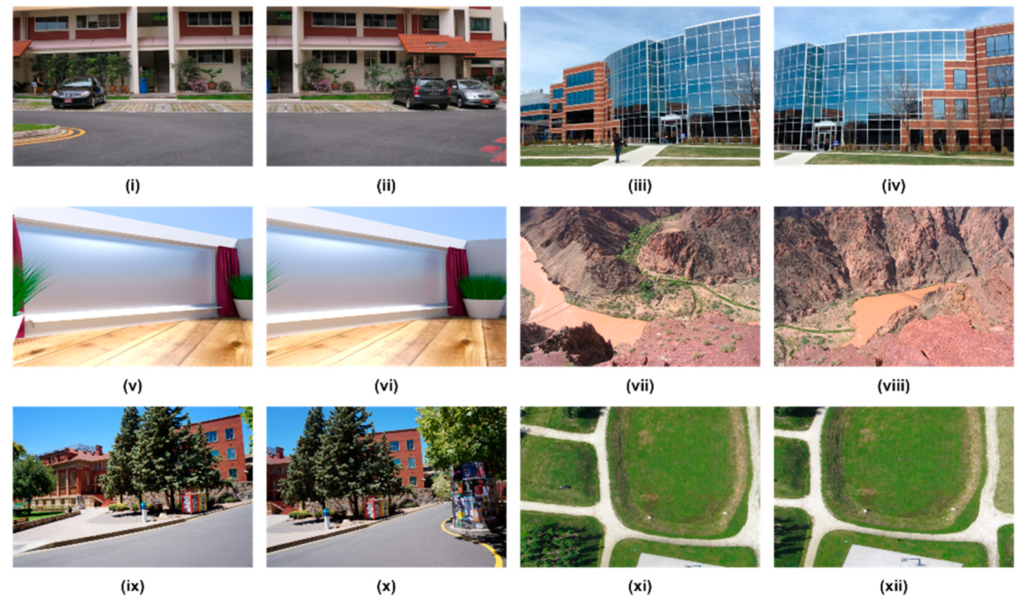
Section 3 provides details about the datasets and methodology used in the study. Section 4 presents results and discusses the outcomes. Finally, the paper is concluded in Section 5.

2. Overview of Feature Detectors and Descriptors

We have made an effort to include an extensive variety of feature detectors and descriptors in terms of universality, approach and age.

2.1. Good Features to Track (GFTT)

The authors of [13] made a minor change to the Harris corner detection algorithm that yields better results than the Harris corner detector. The authors claimed that detected corners are more uniformly distributed across the image.

2.2. SIFT

Lowe [22] proposed one of the most commonly used feature detection and description algorithms, named SIFT. SIFT is invariant to scale, rotation, illumination and viewpoint change; therefore, it can also correctly locate key-points in noisy, cluttered and occluded environments. It identifies interest points in two steps. First, a scale space is generated by continuously smoothing the original image using Gaussian filters that ensure scale invariance. Then, the original image is resized to half size, and again smoothing is performed using a Gaussian filter. This process is repeated. In this manner, an image pyramid is formed, with the reference image at the bottom (level 1). Next, it computes the DoG by subtracting two consecutive scales. Second, interest points are identified by examining the 3 × 3 × 3 neighborhood of any pixel. The image point at which DoG values attain an extrema among all neighbors is considered as a key-point. A description algorithm was also developed for extracting the descriptor of detected key-points. The descriptor is a position-dependent histogram of local image gradient directions in the neighborhood of the key-point.

2.3. MSER

The authors of [36] presented the Maximally Stable Extremal Regions (MSER) algorithm, which is used to detect blobs in images. Ref. [37] presented its updated version, which is computationally faster than the original algorithm. During the procedure, regions are initially recognized using connectivity analysis, and then connected maximum and minimum intensity regions are calculated. Extremal regions are closed by affine or projective transformations as well as changes in illumination. As a result, they are also scale- and rotation-invariant.

2.4. FAST

The FAST corner detector was proposed by [42]. Corner detection is accomplished by first picking a collection of training images then running the FAST algorithm on each image to detect points and then using machine learning to find the optimum detection criterion. The detection criteria are judgements regarding whether or not a pixel is a corner. A decision tree is developed that can accurately categorize all of the corners. After that, the decision tree is transformed into C code, which is subsequently employed as a corner detector. The FAST corner detector is ideal for use in real-time applications, but it is not robust to high degrees of noise.

2.5. SURF

The authors of [38] developed the SURF algorithm, which is a quick and robust approach for feature detection and extraction in the images. The major attraction of the SURF method is its ability to calculate operators fast by applying box filters, enabling its use for real-time applications. For interest point identification, it utilizes Hessian matrix approximation because of its high performance in terms of computing time and accuracy. There are two phases of creating SURF description. The first stage is to establish a repeatable orientation using data from a circular region around the key-point. The SURF descriptor is then extracted from a square area that is aligned to the specified orientation.

2.6. Star Detector (CENSURE)

Agrawal et al. [49] introduced the Center Surround Extremas (CENSURE) detector. It is characterized by two considerations: stability (features invariant to viewpoint changes) and accuracy. First, it uses Hessian–Laplacian method to calculate the maxima. Center surround filters known as bi-level filters are used to approximate the Laplacian. Then, a basic center-surround Haar wavelet is constructed by using this Laplacian; this is the CENSURE response. Then, necessary features are provided by a non-maximal suppression.

2.7. BRIEF

Calonder et al. [51] presented the Binary Robust Independent Elementary Features (BRIEF) descriptor, which is based on binary strings. First, binary strings are computed from image patches, then the individual bits are generated by comparing the brightness of pairs of points along the same lines. BRIEF is fast compared to other descriptors such as SIFT and SURF because SIFT and SURF have a high-dimensional descriptor vector, which requires more time and memory to compute. It can be used with the detectors which do not have their own descriptors.

2.8. DAISY

Tola et al. [52] proposed a local image descriptor named DAISY. DAISY gives very good results in wide-baseline situations in comparison to pixel- and correlation-based approaches. It is faster than other descriptors such as SIFT and the Gradient Location and Orientation Histogram (GLOH). SURF is also efficient, but it introduces artifacts that degrade the matching performance. DAISY computes descriptors at every pixel without inserting any artifacts, which improves its matching performance when used densely. Gaussian convolutions are used for descriptor computation. This method computes descriptors in real time. This speed increase is because DAISY uses sums of convolutions instead of weighted sums used by other descriptors. It uses a circularly symmetrical weighting kernel.

2.9. AGAST

The authors of [70] introduced the Adaptive and Generic Accelerated Segment Test (AGAST) detector, which uses specialized decision trees to enhance the performance. It can be used for any type of scene structure. The optimum trees are identified by using the whole binary configuration space. In FAST, the detector must be trained for a specific scene during the training step, but in AGAST, it adjusts to the environment dynamically while processing an image.

2.10. BRISK

The authors of [53] presented a method, Binary Robust Invariant Scalable Key-Points (BRISK), for key-point detection and description. It uses a novel scale space FAST-based detector for detecting key-points. In this algorithm, key-points are discovered in the image scale-space pyramid. Following that, a circular sampling pattern is created in the vicinity of each detected key-point, which calculates brightness comparisons to form a descriptor string.

2.11. ORB

The authors of [54] developed an Oriented FAST and Rotated BRIEF (ORB) detector and descriptor as an efficient alternative to SIFT and SURF. ORB is a combination of the FAST detector and the BRIEF descriptor, with several enhancements to improve the performance. ORB adds a fast and accurate orientation component to the FAST algorithm. It uses an image pyramid to generate multiscale features. For the descriptor, it steers BRIEF according to the orientation of key-points to make it rotation-invariant.

2.12. FREAK

Alahi et al. [55] presented the Fast Retina Key-Point (FREAK) descriptor, which is based on the retina of the HVS. First, a circular sample grid is used to construct a retinal sampling pattern. The density of points is greater around the center. Then, by comparing brightness across a retinal sampling pattern, a cascade of binary strings is produced employing DoG. A “saccadic search”, which is a human vision-like search, is used to obtain relevant features. Finally, key-point rotation is achieved by summing local gradients over chosen pairs.

2.13. KAZE

The authors of [56] developed a new feature detection and description method in nonlinear scale spaces. Earlier methods detected and described features at various scales by constructing or approximating an image’s Gaussian scale space. However, Gaussian blurring smooths features and noise to the same extent, reducing localization accuracy and distinctiveness. It uses nonlinear diffusion filtering to detect and describe features in a nonlinear scale space. The nonlinear scale space is constructed with the use of efficient Additive Operator Splitting (AOS) methods and variable conductance diffusion. As a result, blurring may be made locally adaptable to the image data, reducing noise and achieving improved localization accuracy and distinctiveness.

2.14. AKAZE

The authors of [57] enhanced the computation cost of KAZE and proposed AKAZE, a faster and multi-scale feature detection and description algorithm. Earlier developed methods for detecting and describing features in nonlinear scale space take more time because constructing the nonlinear scale space is computationally costly. AKAZE employs the Fast Explicit Diffusion (FED) scheme, which is incorporated in a pyramidal structure and speeds up feature detection in nonlinear scale space. By employing FED techniques, nonlinear scale space may be created quicker than any other discretization technique. FED schemes also outperform AOS schemes in terms of ease of implementation and accuracy. AKAZE implements the Modified-Local-Difference Binary (M-LDB) descriptor, which is efficient, scale- and rotation-invariant and uses less memory.

2.15. MSD Detector

Tombari [71] proposed a new detector, Maximal Self-Dissimilarities (MSD), which is able to detect features across multi-modal image pairs. It is based on the intuition that image patches which are very distinct across a reasonably large area of their surroundings are repeatable and distinctive. This idea of contextual self-dissimilarity inverts the essential paradigm of previous successful techniques based on the occurrence of similar rather than different patches. Furthermore, it extended the local self-dissimilarity concept embedded in existing detectors of corner-like interest points to contextual information, resulting in improved repeatability, distinctiveness and localization accuracy.

3. Materials and Methods

To test our framework, we used a variety of datasets (building dataset, tree dataset and classroom dataset) that covered various scene categories with variable degrees of distortion. A subset of input images is depicted in Figure 1.

3.1. Method: Image Stitching Algorithm

Figure 2 depicts the image stitching algorithm used in this work. Image alignment and image blending are the two major components of this approach. In the image alignment phase, a feature detector is used to detect feature points, followed by a feature descriptor to extract descriptors for the detected feature points. The k-nearest neighbor (k-NN) approach is used to match each feature point. False matches may result from automatic feature matching, which can lead to poor alignment; consequently, false matches must be eliminated. The M-estimator sample consensus (MSAC) algorithm is employed to eliminate outliers by reducing matching error. The goal is to collect the most feature points acceptable for transformation. The entire procedure is iterative in nature. Correct matches or inliers are those produced by reducing the matching error. The successful identification of a conjugate feature point on the second image for each corresponding feature point on the first image is defined as a correct match. These inlier points are then utilized to calculate the homography (transformation) between two images. The mathematical relationship described in Equation (1) is used to compute the homography matrix.
X = H X , [ x y 1 ] = [ h 0 h 1 h 2 h 3 h 4 h 5 h 6 h 7 1 ] [ x y 1 ]
Once homography is obtained, the target image is warped (transformed) onto the source image. After the images have been aligned, there may be noticeable seams because of differences in illumination and unintentional camera motions. As a result, image blending is performed to remove the seam.
Table 1 shows feature detectors and descriptors, listed in the order of their development. As shown in the table, some of them are either detectors or descriptors, while others are both. Therefore, to perform a comparative assessment, the best approach is to pair each detector with each descriptor and evaluate its performance. We tested each detector–descriptor combination on a variety of datasets. For each dataset, we use the detector to detect features on the left and right images, and then the paired descriptor was used to extract features. Next, the features were matched using the k-NN matching algorithm. Finally, both the images were stitched using the algorithm described in Figure 2.

3.2. Method: Comparative Analysis

Different feature detector and descriptor combinations were compared in order to choose the best combination for image stitching applications. Inlier ratio, stitched image quality and execution time are the three parameters used for comparison.

3.2.1. Inlier Ratio

Inlier ratio is the ratio of correct matches to the initial matches. This fraction represents the detector–descriptor combination accuracy. A higher inlier ratio value indicates a better detector–descriptor pair. For some image pairs, the value of the inlier ratio may be zero, which indicates that all the initial matches were wrong. In image stitching, at least four correct matched points are required in order to stitch the images. If some combination has less than four correct matched points, we used an inlier ratio equal to zero. The inlier ratio is defined by Equation (2):
Inlier Ratio = number of correct matches number of initial matches
The number of accurate matches has an effect on the quality of the final stitched image since the homography matrix is created using correctly matched points, which are then used in the image alignment stage. As a result, the inlier ratio is one of the most significant parameters to consider when choosing the best detector and descriptor combination.

3.2.2. Stitched Image Quality

The subjective and objective techniques are the two most used techniques for evaluating image quality. In the subjective assessment approach, a number of observers are chosen, and then they are presented a set of photographs. Following that, they are asked to judge image quality based on their assessment. Human inspection is used to give a rating to each image depending on its quality [72]. The objective image quality assessment (IQA) approaches rely on automated algorithms to assess image quality without the need for human intervention [72]. Since subjective assessment techniques differ from person to person, small distortions in the final stitched image cannot be detected. As a result, we employed objective IQA techniques to compare the quality of stitched images in this research. The quality of stitched images generated using different pairs of feature detectors and descriptors was compared based on objective IQA metrics. The objective image quality metrics utilized in this study to assess the quality of stitched images are listed below.

Peak Signal to Noise Ratio

Peak Signal to Noise Ratio (PSNR) is a metric for measuring how different two images are. The PSNR of comparable pixel values is expressed as (Equation (3)):
PSNR = 10 log 10 ( max ( G ( i , j ) , O ( i , j ) ) ) 2 MSE
where G (i, j) and O (i, j) represent the (i, j)th pixel values in the input image and stitched image, respectively. MSE is the mean square error, which is defined as:
MSE = i j ( G ( i , j ) O ( i , j ) ) 2 N
where N is the total number of pixels in each image. A lower MSE value indicates that the difference between two images is low, thus resulting in higher PSNR values.

Structural Similarity Index

The SSIM (Structural Similarity) index is used to determine the similarity of two images. The image that is being assessed is known as the target image, and the image that is used to compare the quality of the target image is known as the reference image. The SSIM index meets the requirements of symmetries, boundedness and having a unique maximum. The luminance measurement is assumed to be qualitatively consistent with Weber’s law, which specifies that the visible change in luminance in the HVS is roughly proportional to the background luminance. Similarly, the contrast measurement follows the HVS by focusing primarily on the relative difference rather than the absolute difference in the contrast. The final SSIM index is a combination of these two values, as well as a structural similarity component determined using brightness and contrast values [73]. SSIM between two images x and y is described as follows (Equation (4)):
SSIM ( x , y ) = ( 2 μ x μ y + C 1 ) ( 2 σ xy + C 2 ) ( μ x 2 + μ y 2 + C 1 ) ( σ x 2 + σ y 2 + C 2 )
where μx and μy represent local means for x and y images, respectively. σx and σy represent standard deviations, and σxy is the cross-covariance for x and y images. The smaller the difference between the structure of x and y, the higher the SSIM index value. If there is no structural difference, SSIM (x, y) = 1.

Feature Similarity Index

The Feature Similarity (FSIM) index is based on how the HVS interprets an image based on its low-level features [74]. Two characteristics, phase congruency (PC) and gradient magnitude (GM), have to be considered in order to calculate the FSIM index. PC and GM are complementary for describing local quality of the image. The FSIM measurement is divided into two components, f 1 ( x ) and f 2 ( x ) , one for PC and one for GM. The measure of similarity in terms of PC 1 ( x ) and is described as (Equation (5)):
S PC ( x ) = 2 PC 1 ( x ) · PC 2 ( x ) + T 1 PC 1 2 ( x ) + PC 2 2 ( x ) + T 1
where T1 is a positive constant.
The measure of similarity in terms of G 1 ( x ) and G 2 ( x ) is described as (Equation (6)):
S G ( x ) = 2 G 1 ( x ) · G 2 ( x ) + T 2 G 1 2 ( x ) + G 2 2 ( x ) + T 2
where T2 is a positive constant.
The combination of and gives the similarity of f 1 ( x ) and f 2 ( x ) , which is represented as:
S L ( x ) = S PC ( x ) · S G ( x )
The FSIM index between f 1 and f 2 is described as (Equation (7)):
FSIM = X Ω S L ( X ) · PC m ( X ) X Ω PC m ( X )
where PC m ( X ) = max ( PC 1 ( x ) · PC 2 ( x ) ) .
The FSIM index was designed to be used with grayscale images or the luminance component of color images. As chrominance information influences the HVS’s interpretation of images, including chrominance information in FSIM for color IQA may result in improved performance. A simple addition to the FSIM framework may be used to accomplish this purpose.
The RGB color images are first transformed to a different color space, where luminance and chrominance may be segregated. The commonly used YIQ color space, in which Y contains luminance information and I and Q provide chrominance information, is utilized to achieve this. The following equation (Equation (8)) may be used to convert from RGB to YIQ space:
[ Y I Q ] = [ 0.299 0.587 0.114 0.596 0.274 0.322 0.211 0.523 0.312 ] [ R G B ]
The similarity between chromatic features is represented as follows:
S I ( x ) = 2 I 1 ( x ) · I 2 ( x ) + T 3 I 1 2 ( x ) + I 2 2 ( x ) + T 3
S Q ( x ) = 2 Q 1 ( x ) · Q 2 ( x ) + T 4 Q 1 2 ( x ) + Q 2 2 ( x ) + T 4
where I 1 ( I 2 ) and Q 1 ( Q 2 ) are the I and Q chromatic channels of the image f 1 ( f 2 ) , respectively. T 3 and T 4 are positive constants. T 3 = T 4 is used for convenience since the I and Q components have almost the same dynamic range.
The chrominance similarity between f I ( x ) and f 2 ( x ) is the obtained by combining the S I ( x ) and S Q ( x ) , which is represented by S C ( x ) as follows:
S C ( x ) = S I ( x ) · S Q ( x )
Finally, by simply adding chromatic information to the FSIM index, it may be easily modified to FSIMC(Equation (9)).
FSIM C = x ϵ Ω S L ( x ) · [ S C ( x ) ] λ PC m ( x ) x ϵ Ω PC m ( x )
where λ > 0 is the parameter that is used to alter the significance of the chromatic components.

Visual Saliency Induced Index

Over the past decade, visual saliency (VS) has been extensively investigated in psychology, neuroscience and computer science to determine which portions of an image would grab the major attention of the HVS. Zhang et al. [75] introduced the visual saliency induced (VSI) index, a simple but highly effective full-reference IQA approach based on VS. The VSI metric between image 1 and image 2 is expressed as follows (Equation (10)):
VSI = X ϵ Ω S ( X ) · VS m ( X ) X ϵ Ω VS m ( X )
where Ω denotes the complete spatial domain S ( X ) = S VS ( X ) · [ S G ( X ) ] α · [ S C ( X ) ] β .
  • S VS ( X ) is a component of visual saliency similarity between two images.
  • S G ( X ) is the similarity component of gradient modulus between two images.
  • S C ( X ) is the component of chrominance similarity between two images.
    VS m ( X ) = max ( VS 1 ( x ) · VS 2 ( x ) )
VS 1 ( x ) and VS 2 ( x ) are visual saliency maps of image1 and image2, respectively.

3.2.3. Execution Time

The overall time required to identify, match and stitch the input images is referred to as the execution time. The execution time is a significant consideration when choosing an image stitching method for real-time applications. For some detector–descriptor pairs, either correct matches are zero or less than four. Therefore, for those pairs, execution time has no meaning because we consider execution time as total time from detection to final stitched image generation. In order to quantitatively compare those pairs with other pairs, we used a large dummy value for the execution time of those pairs. In this study, set this dummy value equal to 100 s.
The abovementioned IQA measures are used to assess the stitched image’s quality. The quality of the stitched image produced from every feature detector–descriptor pair is assessed by comparing the quality of the overlapping area of the input and the final stitched image. As shown in Figure 3, the overlapping regions of each left image (L) and right image (R) are compared to the overlapping areas of the final stitched image. In Figure 3, the overlapping area in the left image, right image and stitched image is represented by Lo, Ro and So, respectively. Quality metrics were calculated for each image pair and each detector–descriptor pair. In order to acquire quality metrics, the overlapping region So was compared to Lo and Ro individually, and then the mean value was computed. Figure 3 illustrates the entire workflow for evaluating the performance of the feature detector–descriptor combination for image stitching.

3.3. Method: Rank Computation

A rank is assigned to each combination of detector and descriptor based on the inlier ratio, stitching image quality and execution time. For comparison, six metrics are available: inlier ratio, execution time, PSNR, SSIM, FSIM and VSI. The rank computation algorithm has been adopted from [67,76]. The methodology for rank computation is outlined below:
  • For method m (detector–descriptor pair) with dataset d and metric t, find the positional rank Pm,d,t by sorting the metric values (a low value denotes better positional rank for execution time, while a high value denotes better positional rank for all other metrics).
  • Compute the average rank of m for dataset d, over all metrics: R m , d = 1 N t t P m , d , t . Here, Nt denotes the number of metrics.
  • Compute the positional rank of each method m for each dataset d based on the value of Rm,d, by sorting Rm,d in ascending order (low Rm,d indicates better positional rank). If two successive rankings have extremely close values within a given threshold T, then the same positional rank is assigned. As a result, the positional ranks start with 1 and increment when two successive ranks differ by a value greater than the threshold T. The positional rank is denoted by Pm,d. For the rank computation, we have selected T = 0.05 × SD, where SD is standard deviation.
  • Find the average rank across all datasets: R m = 1 N d d P m ,   d . Here, Nd represents the number of datasets.
  • Finally, determine Pm, the positional rank across datasets by sorting Rm in ascending order.
Using the abovementioned algorithm, we calculated the rank of each method m (detector and descriptor combination). We computed the rank of each method m for datasets 1, 2 and 3 separately.

4. Results and Discussion

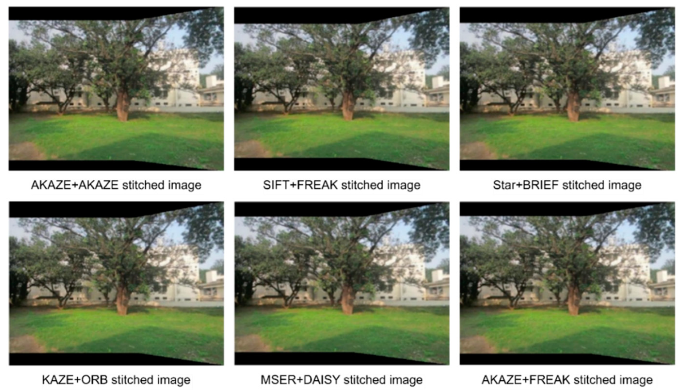
In this study, we analyzed a total 85 feature detector–descriptor combinations pairs. It is not possible to show outputs of all combinations here; therefore, we show stitched image outputs of the top six combinations in each dataset category. Figure 4 shows the output stitched images of the top six combinations which produce better quality of stitched images in comparison to all other combinations for dataset 1. Upon close examination of the stitched images, it can be observed that AKAZE + AKAZE combination gives the best-quality image, which is further verified by the objective IQA metrics.
Table 2 shows the inlier ratio obtained using different combinations of feature detector and descriptors for dataset 1. Table 3, Table 4, Table 5 and Table 6 presents the values of PSNR, SSIM, FSIM and VSI obtained using various combinations of detector–descriptor pairs for dataset 1. Table 7 shows execution time of different detector–descriptor-based algorithms for dataset 1. In all the tables, some entries are marked as NC. NC stands for “not compatible”, i.e., that particular descriptor is not compatible with combined detector.
For dataset 1, ORB + SIFT has a very good inlier ratio, but the quality of the stitched image is poor in comparison to other pairs. This pair has poor quality of stitched images despite its very good inlier ratio because in order to obtain a better-quality image, the matched points should be spread into the image, but for this pair, matched points are clustered. It also takes more execution time. ORB + BRISK also has a very good inlier ratio, but the quality of the stitched image is poor because of the low number of matched points. It has better execution time than ORB + SIFT, which may be because the BRISK descriptor takes less time to extract descriptors than SIFT. AKAZE + SIFT and AKAZE + DAISY both have very good inlier ratio, a little lower than ORB + BRISK. The quality of stitched image obtained using both the combinations is also good because they have sufficient matches. AKAZE + AKAZE also has a good inlier ratio, and the quality of stitched image is also superior to all other combinations. This is because the number of matches is good and are well spread over the image. It also takes less execution time. GFTT + BRISK, AKAZE + ORB, AKAZE + BRISK and FAST + BRISK all have average inlier ratio, but the quality of stitched image is very good. This may be because these combinations produce more false matches, which reduces the inlier ratio, and the correct matches are well spread over the image, which leads to a better quality stitched image. BRISK + ORB and SIFT + FREAK have low inlier ratio and degraded quality of the stitched image. Overall, AKAZE + AKAZE has very good inlier ratio, generating very good stitched images with relatively short execution time (Table 7), which implies that AKAZE + AKAZE is best suited for stitching dataset 1.
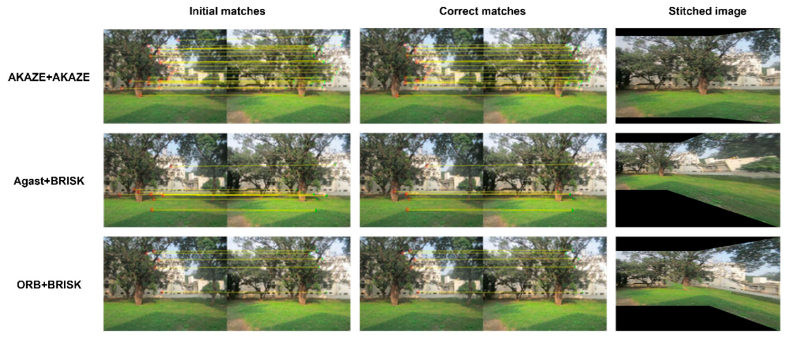
Figure 5 shows results obtained using AKAZE + AKAZE, BRISK + ORB and SIFT + FREAK combinations for dataset 1. The first column in each row displays the initial matches for that particular detector–descriptor combination, and the second column shows the correct matches for the detector–descriptor pair. The last column shows the stitched image obtained using that particular combination.
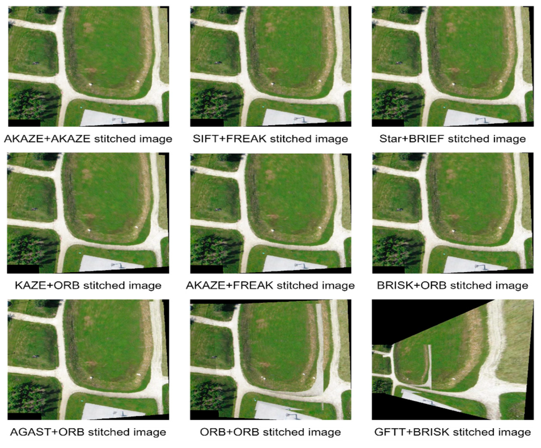
Figure 6 shows the output stitched images of the top six combinations, which produces a better quality of stitched image in comparison to all other combinations for dataset 2. Again, it is observed that the AKAZE + AKAZE combination gives the best-quality image.
Table 8 shows the inlier ratio obtained using different combinations of feature detector and descriptors for dataset 2. Table 9, Table 10, Table 11 and Table 12 presents the values of PSNR, SSIM, FSIM and VSI obtained using various combinations of detector–descriptor pairs for dataset 2. It is observed that the AKAZE + AKAZE combination has highest values of quality metrics for dataset 2.
Table 13 shows execution time of different detector–descriptor-based algorithms for dataset 2.
For dataset 2, AKAZE + BRISK and ORB + BRISK both have very good inlier ratio, but the quality of the stitched image is poor; this is because they have a smaller number of correct matched points, which affected the homography metric that in turn resulted into degraded quality of the stitched image. SURF + BRISK and ORB + SIFT also have a very good inlier ratio, but the quality of stitched image is poor; this is because the matched points are not well spread in the image. AKAZE + AKAZE has a very good inlier ratio, and stitched image quality is also very good. This is because AKAZE + AKAZE has a good number of matched points that are well spread across the image. KAZE + ORB, SIFT + FREAK, KAZE + FREAK and AKAZE + FREAK have average inlier ratio in comparison to other combinations, but the quality of stitched image is good. The inlier ratio is low because of the higher number of initial matched points and smaller number of correct matched points in comparison to initial matched points, but correct matched points are sufficient to obtain an accurate homography metric, which in turn gives a good quality of stitched image. AGAST + BRISK has low inlier ratio and poor stitched image quality because of a smaller number of matched points. SIFT + BRIEF and AKAZE + SIFT also generate a poor quality of stitched image because of the low inlier ratio. Once again, AKAZE + AKAZE generated a very good quality of stitched image with relatively short execution time (Table 13), which makes AKAZE + AKAZE the best choice for stitching dataset 2, which contains outdoor scenes with irregular features such as trees.
Figure 7 shows results obtained using AKAZE + AKAZE, AGAST + BRISK and ORB + BRISK combinations for dataset 2. Each row in the figure presents a detector–descriptor combination, where the first column illustrates the initial matches for that particular pair, the second column shows the correct matches, and the last column exhibits the stitched image produced using that combination.
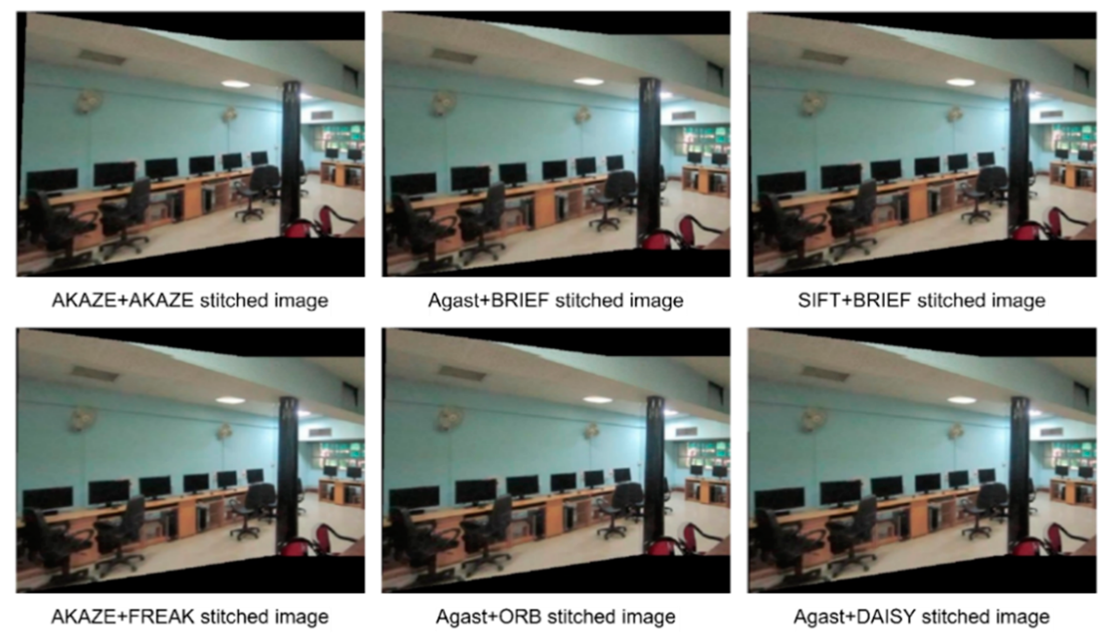
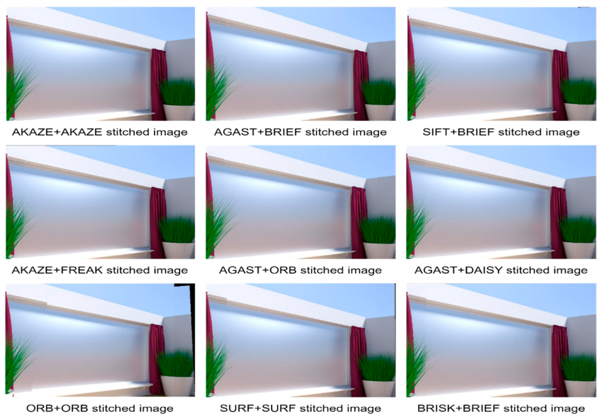
Figure 8 shows the output stitched images of the top six combinations which produce a better quality of stitched image in comparison to all other combinations for dataset 3. It is observed that the AKAZE + AKAZE combination gives the best-quality image. We found one more combination, AGAST + BRIEF which also gives a better quality of stitched image.
Table 14 shows the inlier ratio, obtained using different combinations of feature detector and descriptors for dataset 3. Table 15, Table 16, Table 17 and Table 18 presents the values of PSNR, SSIM, FSIM and VSI obtained using various combinations of detector–descriptor pairs for dataset 3. It is observed that the AKAZE + AKAZE combination has the highest values of quality metrics for dataset 3. It is observed that the AGAST + BRIEF combination also gives a very good quality of stitched image.
For dataset 3, MSD + BRISK, ORB + BRISK, SURF + BRISK and GFTT + BRISK have very good inlier ratio, but the quality of stitched image is poor because of a smaller number of matched points. This also implies that the BRISK descriptor is not suitable for stitching indoor scene images. AKAZE + SIFT has a good inlier ratio, but the quality of stitched image is poor because matched points are not well spread across the image. AKAZE + AKAZE has a good inlier ratio, and the stitched image quality is also very good because it has sufficient number of matched points that are well spread across the images. SIFT + FREAK has an average inlier ratio in comparison to other combinations, and its quality is poor because it has a smaller number of matched points. AGAST + DAISY has average inlier ratio, but the quality of stitched image is very good because of the sufficient number of correct matches. SIFT + BRIEF, AKAZE + FREAK, AGAST + BRIEF and MSD + FREAK generate a good quality of stitched images because the correct matched points are well spread across the image. AGAST + BRISK, ORB + SIFT and KAZE + ORB have poor inlier ratio and poor quality of stitched image. This is because they have very a smaller number of matched points. The inlier ratio of AKAZE + ORB, KAZE + FREAK and FAST + BRISK is low, and the quality of stitched image is not good because of a smaller number of matched points. Overall, AKZE + AKAZE and AGAST + BRIEF generate a very good quality of stitched image, and both are computationally faster (Table 19) for stitching dataset 3 images. Therefore, it can be concluded that AKAZE + AKZE and AGAST + BRIEF are the best choices for stitching indoor scene images.
Figure 9 shows results obtained using AKAZE + AKAZE, AGAST + BRIEF, ORB + BRISK and GFTT + BRISK combinations for dataset 3. In the figure, each row represents a unique detector–descriptor combination. The first column demonstrates the initial matches for that particular pair, while the second column showcases the correct matches. The last column displays the resulting stitched image obtained using that specific combination.
We also considered six publicly available datasets for image stitching. The input images of the dataset used and the generated stitched output images are given in Appendix A. We examined a pair of deep learning algorithms for image stitching that were recently introduced in the literature. Appendix B contains the results obtained using these deep learning algorithms.
Table 20 (dataset 1 column) shows the top ten methods (detector and descriptor combination) for dataset 1. AKAZE + AKAZE is top ranked for dataset 1, and after that BRISK + FREAK and AKAZE + ORB are at second position. Table 20 (dataset 2 column) presents the top ten methods for dataset 2. AKAZE + AKAZE performs the best in dataset 2 and hence ranks first. SIFT + FREAK and Star + BRIEF are at the second position. Table 20 (dataset 3 column) shows the top ten methods for dataset 3. AKAZE + AKAZE is at top position for dataset 3, and AGAST + BRIEF secures the second position. SIFT + BRIEF is in the third position.
Finally, the ranking may be adjusted by weighting particular metrics while averaging the results. In future, different weights can be assigned to each metric depending upon the requirements; for example, in real time applications, we can compromise with quality for shorter execution time; therefore, we can assign higher weight to execution time in comparison to quality metrics. In virtual tour applications, quality is important, so we can assign quality metrics higher weight than execution time.

5. Conclusions

A comprehensive comparison of fifteen notable feature detection and description techniques for image stitching was carried out in the study. The following are some of the contributions made by this research: (1) The evaluations give a better picture of how feature detectors and descriptors work across a variety of image datasets; (2) cumulative comparisons for a complete set of 85 detector–descriptor pairs were performed over a number of datasets; and (3) a rank was assigned to each detector and descriptor pair for each dataset, which shows the relative performance of the detector and descriptor for that particular type of dataset. Overall, it was identified that the AKAZE detector paired with the AKAZE descriptor outperforms all other combinations for all types of selected datasets. The AGAST detector combined with the BRIEF descriptor also performs very well for dataset 3 containing indoor scenes.
In future, we can include more datasets, and a study of detectors and descriptors can be performed by varying parameters of each detector and descriptor. The ranking can also be made more application-specific by assigning suitable weights to each metric.

Author Contributions

Conceptualization, S.K.S. and K.J.; methodology, S.K.S.; software, S.K.S.; validation, S.K.S. and K.J.; formal analysis, S.K.S.; investigation, S.K.S.; writing—original draft preparation, S.K.S.; writing—review and editing, S.K.S. and A.K.S.; visualization, S.K.S. and A.K.S.; supervision, K.J. and A.K.S. All authors have read and agreed to the published version of the manuscript.

Funding

This research received no external funding.

Institutional Review Board Statement

Not applicable.

Informed Consent Statement

Not applicable.

Data Availability Statement

The data presented in this study are available on request from the corresponding author.

Conflicts of Interest

The authors declare no conflict of interest.

Appendix A

We also considered six publicly available datasets: (1) apartment dataset [77], (2) MATLAB dataset (MATLAB vision toolbox dataset), (3) synthetic dataset [78], (4) river dataset (VLFeat dataset), (5) garden dataset [77] and (6) UAV dataset [79]. Input images used from these datasets are shown in Figure A1. The stitched images obtained using different combinations of feature detectors and descriptors from these datasets are shown in Figure A2, Figure A3, Figure A4, Figure A5, Figure A6 and Figure A7.
Figure A1. Input datasets: (i) and (ii) apartment dataset image pair; (iii) and (iv) MATLAB dataset image pair; (v) and (vi) synthetic dataset image pair; (vii) and (viii) river dataset image pair; (ix) and (x) garden dataset image pair; (xi) and (xii) UAV dataset.
Applsci 13 06015 g0a1
Figure A2. Image stitching outputs obtained for different feature detector–descriptor combinations for apartment dataset.
Applsci 13 06015 g0a2
Figure A3. Image stitching outputs obtained for different feature detector–descriptor combinations for MATLAB dataset.
Applsci 13 06015 g0a3
Figure A4. Image stitching outputs obtained for different feature detector–descriptor combinations for synthetic dataset.
Applsci 13 06015 g0a4
Figure A5. Image stitching outputs obtained for different feature detector–descriptor combinations for river dataset.
Applsci 13 06015 g0a5
Figure A6. Image stitching outputs obtained for different feature detector–descriptor combinations for garden dataset.
Applsci 13 06015 g0a6
Figure A7. Image stitching outputs obtained for different feature detector–descriptor combinations for UAV dataset.
Applsci 13 06015 g0a7
Figure A2 shows a subset of output stitched images obtained using various detector–descriptor combinations for the apartment dataset. The first and second rows show a subset of stitched images obtained using different detector–descriptor combinations, which produces a good quality of stitched image in comparison to all other combinations. The third row shows a subset of stitched outputs using different detector–descriptor combinations, which produces poor quality of stitched images. It was observed that AKAZE + AKAZE produced a better quality of stitched image in comparison to all other combinations.
In Figure A3, a collection of stitched images generated from a range of detector–descriptor combinations on the MATLAB dataset is displayed. The first and second rows exhibit examples of high-quality stitched images, while the third row showcases a sample of poorly stitched outputs resulting from different detector–descriptor combinations. It was noted that the AKAZE + AKAZE combination produced the highest quality stitched image compared to all other combinations.
Figure A4 displays a variety of stitched images created from a selection of detector–descriptor combinations on the synthetic dataset. The first and second rows illustrate instances of well-stitched images, while the third row features a subset of poorly stitched outputs that resulted from various detector–descriptor combinations. The AKAZE + AKAZE and AGAST + BRIEF combinations were observed to produce the highest quality stitched images compared to all other combinations.
Figure A5 showcases a range of stitched output images that were generated using various detector–descriptor combinations on the river dataset. The first and second rows display a subset of well-stitched outputs that outperformed all other combinations in terms of quality. Conversely, the third row exhibits a selection of poorly stitched outputs resulting from different detector–descriptor combinations. It was noted that the AKAZE + AKAZE and SURF + SURF combinations produced the highest quality stitched images among all the combinations tested.
In Figure A6, a variety of stitched output images obtained from different detector–descriptor combinations on the garden dataset are showcased. The first and second rows exhibit a subset of well-stitched outputs that displayed superior quality compared to all other combinations. Conversely, the third row features a subset of poorly stitched outputs resulting from various detector–descriptor combinations. It was observed that the AKAZE + AKAZE combination produced the highest quality stitched image among all the combinations tested.
Figure A7 displays a selection of stitched output images that were produced using different detector–descriptor combinations on the UAV dataset. The first and second rows exhibit a subset of well-stitched outputs that demonstrated superior quality compared to all other combinations. However, the third row features a subset of poorly stitched outputs resulting from various detector–descriptor combinations, as evidenced by the outputs in the last row. Among all the combinations tested, it was observed that the AKAZE + AKAZE produced the highest quality stitched image.

Appendix B

We evaluated two recent advanced image stitching algorithms that are based on deep learning techniques. These algorithms are: (1) A view-free image stitching network [80] and (2) unsupervised deep image stitching [81]. We utilized both of these algorithms to stitch images from all datasets under consideration. Figure A8 showcases the stitched images obtained using the view-free image stitching network algorithm, while Figure A9 presents those obtained through unsupervised deep image stitching. It was observed that while the deep learning-based algorithms produced acceptable results for synthetic datasets, the stitched images obtained using these algorithms for real-world datasets suffered from different types of distortions such as misalignment and projective distortions.
Figure A8. Image stitching outputs obtained using view-free image stitching network for different datasets: (a) stitched image dataset 1; (b) stitched image dataset 2; (c) stitched image dataset 3; (d) stitched image apartment dataset; (e) stitched image MATLAB dataset; (f) stitched image synthetic dataset; (g) stitched image river dataset; (h) stitched image garden dataset; (i) stitched image UAV dataset.
Applsci 13 06015 g0a8
Figure A9. Image stitching outputs obtained using unsupervised deep image stitching algorithm for different datasets: (a) stitched image dataset 1; (b) stitched image dataset 2; (c) stitched image dataset 3; (d) stitched image apartment dataset; (e) stitched image MATLAB dataset; (f) stitched image synthetic dataset; (g) stitched image river dataset; (h) stitched image garden dataset; (i) stitched image UAV dataset.
Applsci 13 06015 g0a9

References

  1. Wang, J.; Fang, J.; Liu, X.; Zhao, D.; Xiao, Q. A fast mosaic method for airborne images: The new Template-Convolution Speed-Up Robust Features (TSURF) algorithm. Int. J. Remote Sens. 2014, 35, 5959–5970. [Google Scholar] [CrossRef]
  2. Nguyen, T.L.; Byun, Y.; Han, D.; Huh, J. Efficient seamline determination for UAV image mosaicking using edge detection. Remote Sens. Lett. 2018, 9, 763–769. [Google Scholar] [CrossRef]
  3. Kwokjet, R.; Curlander, J.C.; Pang, S.S. An automated system for mosaicking spaceborne SAR imagery. Int. J. Remote Sens. 1990, 11, 209–223. [Google Scholar] [CrossRef]
  4. Rivard, B.; Toutin, T. A Mosaic of Airborne SAR Imagery for Geological Mapping in Rolling Topography. Can. J. Remote Sens. 1995, 21, 75–78. [Google Scholar] [CrossRef]
  5. Majumdar, J.; Vanathy, B.; Varshney, N.; Rao, D.R.; Jalan, U.; Girish, R. Image Mosaicing from Video Sequences. IETE J. Res. 2002, 48, 303–310. [Google Scholar] [CrossRef]
  6. Gheisari, M.; Sabzevar, M.F.; Chen, P.; Irizzary, J. Integrating BIM and Panorama to Create a Semi-Augmented-Reality Experience of a Construction Site. Int. J. Constr. Educ. Res. 2016, 12, 303–316. [Google Scholar] [CrossRef]
  7. Morevec, H.P. Towards automatic visual obstacle avoidance. In Proceedings of the 5th International Joint Conference on Artificial Intelligence, Cambridge, MA, USA, 22–25 August 1977; p. 584. [Google Scholar]
  8. Förstner, W.; Gülch, E. A fast operator for detection and precise location of distinct points, corners and centres of circular features. In Proceedings of the ISPRS Intercommission Conference on Fast Processing of Photogrammetric Data, Interlaken, Switzerland, 2–4 June 1987; pp. 281–305. [Google Scholar]
  9. Harris, C.; Stephens, M. A combined corner and edge detector. In Proceedings of the 4th Alvey Vision Conference, Manchester, UK, 31 August–2 September 1988; p. 151. [Google Scholar]
  10. Tomasi, C.; Kanade, T. Detection and Tracking of Point Features. Int. J. Comput. Vis. 1991, 9, 137–154. [Google Scholar] [CrossRef]
  11. Heitger, F.; Rosenthaler, L.; Von Der Heydt, R.; Peterhans, E.; Kübler, O. Simulation of neural contour mechanisms: From simple to end-stopped cells. Vis. Res. 1992, 32, 963–981. [Google Scholar] [CrossRef]
  12. Förstner, W. A framework for low level feature extraction. In Proceedings of the 3rd European Conference on Computer Vision, Stockholm, Sweden, 2–6 May 1994; pp. 383–394. [Google Scholar]
  13. Shi, J.; Tomasi, C. Good features to track. In Proceedings of the Conference on Computer Vision and Pattern Recognition, Seattle, WA, USA, 21–23 June 1994; pp. 593–600. [Google Scholar] [CrossRef]
  14. Lindeberg, T. Junction detection with automatic selection of detection scales and localization scales. In Proceedings of the 1st International Conference on Image Processing, Austin, TX, USA, 13–16 November 1994; Volume 1, pp. 924–928. [Google Scholar] [CrossRef]
  15. Wang, H.; Brady, M. Real-time corner detection algorithm for motion estimation. Image Vis. Comput. 1995, 13, 695–703. [Google Scholar] [CrossRef]
  16. Smith, S.M.; Brady, J.M. SUSAN—A New Approach to Low Level Image Processing. Int. J. Comput. Vis. 1997, 23, 45–78. [Google Scholar] [CrossRef]
  17. Hall, D.; Leibe, B.; Schiele, B. Saliency of Interest Points under Scale Changes. In Proceedings of the British Machine Vision Conference (BMVC’02), Cardiff, UK, 2–5 September 2002; pp. 646–655. [Google Scholar]
  18. Lindeberg, T. Feature Detection with Automatic Scale Selection. Int. J. Comput. Vis. 1998, 30, 79–116. [Google Scholar] [CrossRef]
  19. Mikolajczyk, K.; Schmid, C. Indexing based on scale invariant interest points. Proc. IEEE Int. Conf. Comput. Vis. 2001, 1, 525–531. [Google Scholar] [CrossRef]
  20. Schmid, C.; Mohr, R.; Bauckhage, C. Comparing and evaluating interest points. In Proceedings of the 6th International Conference on Computer Vision (IEEE Cat. No.98CH36271), Bombay, India, 7 January 1998; pp. 230–235. [Google Scholar] [CrossRef]
  21. Schmid, C.; Mohr, R.; Bauckhage, C. Evaluation of Interest Point Detectors. Int. J. Comput. Vis. 2000, 37, 151–172. [Google Scholar] [CrossRef]
  22. Lowe, D.G. Object recognition from local scale-invariant features. Proc. IEEE Int. Conf. Comput. Vis. 1999, 2, 1150–1157. [Google Scholar] [CrossRef]
  23. Brown, M.; Lowe, D.G. Recognising panoramas. In Proceedings of the 9th International Conference on Computer Vision, Nice, France, 13–16 October 2003; Volume 2, pp. 1218–1225. [Google Scholar] [CrossRef]
  24. Brown, M.; Lowe, D.G. Automatic panoramic image stitching using invariant features. Proc. Int. J. Comput. Vis. 2007, 74, 59–73. [Google Scholar] [CrossRef]
  25. Zhu, J.; Ren, M. Image mosaic method based on SIFT features of line segment. Comput. Math. Methods Med. 2014, 2014, 926312. [Google Scholar] [CrossRef]
  26. Qu, Z.; Lin, S.P.; Ju, F.R.; Liu, L. The Improved Algorithm of Fast Panorama Stitching for Image Sequence and Reducing the Distortion Errors. Math. Probl. Eng. 2015, 2015, 428076. [Google Scholar] [CrossRef]
  27. Mikolajczyk, K.; Schmid, C. A performance evaluation of local descriptors. IEEE Trans. Pattern Anal. Mach. Intell. 2005, 27, 1615–1630. [Google Scholar] [CrossRef]
  28. Zuliani, M.; Kenney, C.; Manjunath, B.S. A mathematical comparison of point detectors. In Proceedings of the Conference on Computer Vision and Pattern Recognition Workshop, Washington, DC, USA, 27 June–2 July 2004. [Google Scholar] [CrossRef]
  29. Gao, J.; Huang, X.; Liu, B. A quick scale-invariant interest point detecting approach. Mach. Vis. Appl. 2010, 21, 351–364. [Google Scholar] [CrossRef]
  30. Feng, Y.; Ren, J.; Jiang, J.; Halvey, M.; Jose, J.M. Effective venue image retrieval using robust feature extraction and model constrained matching for mobile robot localization. Mach. Vis. Appl. 2011, 23, 1011–1027. [Google Scholar] [CrossRef]
  31. Liao, K.; Liu, G.; Hui, Y. An improvement to the SIFT descriptor for image representation and matching. Pattern Recognit. Lett. 2013, 34, 1211–1220. [Google Scholar] [CrossRef]
  32. Wu, J.; Cui, Z.; Sheng, V.S.; Zhao, P.; Su, D.; Gong, S. A comparative study of SIFT and its variants. Meas. Sci. Rev. 2013, 13, 122–131. [Google Scholar] [CrossRef]
  33. Mikolajczyk, K.; Schmid, C. Scale & Affine Invariant Interest Point Detectors. Int. J. Comput. Vis. 2004, 60, 63–86. [Google Scholar] [CrossRef]
  34. Mikolajczyk, K.; Tuytelaars, T.; Schmid, C.; Zisserman, A.; Matas, J.; Schaffalitzky, F.; Kadir, T.; Van Gool, L. A Comparison of Affine Region Detectors. Int. J. Comput. Vis. 2005, 65, 43–72. [Google Scholar] [CrossRef]
  35. Moreels, P.; Perona, P. Evaluation of features detectors and descriptors based on 3D objects. In Proceedings of the 10th International Conference on Computer Vision (ICCV’05), Beijing, China, 17–21 October 2005; Volume 1, pp. 800–807. [Google Scholar] [CrossRef]
  36. Matas, J.; Chum, O.; Urban, M.; Pajdla, T. Robust wide-baseline stereo from maximally stable extremal regions. Image Vis. Comput. 2004, 22, 761–767. [Google Scholar] [CrossRef]
  37. Nistér, D.; Stewénius, H. Linear Time Maximally Stable Extremal Regions. In Lecture Notes in Computer Science (Including Subseries Lecture Notes in Artificial Intelligence and Lecture Notes in Bioinformatics); Springer: Berlin/Heidelberg, Germany, 2008; Volume 5303, pp. 183–196. ISBN 3540886850. [Google Scholar]
  38. Bay, H.; Tuytelaars, T.; Gool, L. Van SURF: Speeded Up Robust Features. In Lecture Notes in Computer Science (Including Subseries Lecture Notes in Artificial Intelligence and Lecture Notes in Bioinformatics); Springer: Berlin/Heidelberg, Germany, 2006; Volume 3951, pp. 404–417. [Google Scholar] [CrossRef]
  39. Niu, J.; Yang, F.; Shi, L. Improved method of automatic image stitching based on SURF. In Proceedings of the 1st International Symposium on Future Information and Communication Technologies for Ubiquitous HealthCare (Ubi-HealthTech), Jinhua, China, 1–3 July 2013. [Google Scholar] [CrossRef]
  40. Zhu, L.; Wang, Y.; Zhao, B.; Zhang, X. A fast image stitching algorithm based on improved SURF. In Proceedings of the 10th International Conference on Computational Intelligence and Security, Kunming, China, 15–16 November 2014; pp. 171–175. [Google Scholar] [CrossRef]
  41. Yang, Z.; Shen, D.; Yap, P.-T. Image mosaicking using SURF features of line segments. PLoS ONE 2017, 12, e0173627. [Google Scholar] [CrossRef]
  42. Rosten, E.; Drummond, T. Machine Learning for High-Speed Corner Detection. In Lecture Notes in Computer Science (Including Subseries Lecture Notes in Artificial Intelligence and Lecture Notes in Bioinformatics); Springer: Berlin/Heidelberg, Germany, 2006; Volume 3951, pp. 430–443. [Google Scholar] [CrossRef]
  43. Tuytelaars, T.; Mikolajczyk, K. Local invariant feature detectors: A survey. Found. Trends Comput. Graph. Vis. 2007, 3, 177–280. [Google Scholar] [CrossRef]
  44. Li, J.; Allinson, N.M. A comprehensive review of current local features for computer vision. Neurocomputing 2008, 71, 1771–1787. [Google Scholar] [CrossRef]
  45. Govender, N. Evaluation of feature detection algorithms for structure from motion. In Proceedings of the 3rd Robotics and Mechatronics Symposium (ROBMECH 2009), Pretoria, South Africa, 8–10 November 2009; p. 4. [Google Scholar]
  46. Gil, A.; Mozos, O.M.; Ballesta, M.; Reinoso, O. A comparative evaluation of interest point detectors and local descriptors for visual SLAM. Mach. Vis. Appl. 2009, 21, 905–920. [Google Scholar] [CrossRef]
  47. Hartmann, J.; Klussendorff, J.H.; Maehle, E. A comparison of feature descriptors for visual SLAM. In Proceedings of the European Conference on Mobile Robots, Barcelona, Spain, 25–27 September 2013; pp. 56–61. [Google Scholar] [CrossRef]
  48. Urban, S.; Weinmann, M. Finding a Good Feature Detector-Descriptor Combination for the 2D Keypoint-Based Registration of TLS Point Clouds. ISPRS Ann. Photogramm. Remote Sens. Spat. Inf. Sci. 2015, 2, 121–128. [Google Scholar] [CrossRef]
  49. Agrawal, M.; Konolige, K.; Blas, M.R. CenSurE: Center Surround Extremas for Realtime Feature Detection and Matching. In Lecture Notes in Computer Science (Including Subseries Lecture Notes in Artificial Intelligence and Lecture Notes in Bioinformatics); Springer: Berlin/Heidelberg, Germany, 2008; Volume 5305, pp. 102–115. [Google Scholar] [CrossRef]
  50. Willis, A.; Sui, Y. An algebraic model for fast corner detection. In Proceedings of the 12th International Conference on Computer Vision, Kyoto, Japan, 29 September–2 October 2009; pp. 2296–2302. [Google Scholar] [CrossRef]
  51. Calonder, M.; Lepetit, V.; Strecha, C.; Fua, P. BRIEF: Binary Robust Independent Elementary Features. In Lecture Notes in Computer Science (Including Subseries Lecture Notes in Artificial Intelligence and Lecture Notes in Bioinformatics); Springer: Berlin/Heidelberg, Germany, 2010; Volume 6314, pp. 778–792. [Google Scholar] [CrossRef]
  52. Tola, E.; Lepetit, V.; Fua, P. DAISY: An efficient dense descriptor applied to wide-baseline stereo. IEEE Trans. Pattern Anal. Mach. Intell. 2010, 32, 815–830. [Google Scholar] [CrossRef] [PubMed]
  53. Leutenegger, S.; Chli, M.; Siegwart, R.Y. BRISK: Binary Robust invariant scalable keypoints. In Proceedings of the International Conference on Computer Vision, Barcelona, Spain, 6–13 November 2011; pp. 2548–2555. [Google Scholar] [CrossRef]
  54. Rublee, E.; Rabaud, V.; Konolige, K.; Bradski, G. ORB: An efficient alternative to SIFT or SURF. In Proceedings of the International Conference on Computer Vision, Barcelona, Spain, 6–13 November 2011; pp. 2564–2571. [Google Scholar] [CrossRef]
  55. Alahi, A.; Ortiz, R.; Vandergheynst, P. FREAK: Fast retina keypoint. In Proceedings of the Conference on Computer Vision and Pattern Recognition (CVPR), Providence, RI, USA, 16–21 June 2012; pp. 510–517. [Google Scholar] [CrossRef]
  56. Alcantarilla, P.F.; Bartoli, A.; Davison, A.J. KAZE Features. In Lecture Notes in Computer Science (Including Subseries Lecture Notes in Artificial Intelligence and Lecture Notes in Bioinformatics); Springer: Berlin/Heidelberg, Germany, 2012; Volume 7577, pp. 214–227. [Google Scholar] [CrossRef]
  57. Alcantarilla, P.F.; Nuevo, J.; Bartoli, A. Fast explicit diffusion for accelerated features in nonlinear scale spaces. In Proceedings of the Tilo Burghardt, Dima Damen, Walterio W. Mayol-Cuevas, Majid Mirmehdi: British Machine Vision Conference, BMVC 2013, Bristol, UK, 9–13 September 2013. [Google Scholar] [CrossRef]
  58. Sharma, S.K.; Jain, K. Image Stitching using AKAZE Features. J. Indian Soc. Remote Sens. 2020, 48, 1389–1401. [Google Scholar] [CrossRef]
  59. Ghosh, D.; Kaabouch, N. A survey on image mosaicing techniques. J. Vis. Commun. Image Represent. 2016, 34, 1–11. [Google Scholar] [CrossRef]
  60. Wang, Z.; Yang, Z. Review on image-stitching techniques. Multimed. Syst. 2020, 26, 413–430. [Google Scholar] [CrossRef]
  61. LYU, W.; ZHOU, Z.; CHEN, L.; ZHOU, Y. A survey on image and video stitching. Virtual Real. Intell. Hardw. 2019, 1, 55–83. [Google Scholar] [CrossRef]
  62. Megha, V.; Rajkumar, K.K. A Comparative Study on Different Image Stitching Techniques. Int. J. Eng. Trends Technol. 2022, 70, 44–58. [Google Scholar] [CrossRef]
  63. Heinly, J.; Dunn, E.; Frahm, J.M. Comparative Evaluation of Binary Features. In Lecture Notes in Computer Science (Including Subseries Lecture Notes in Artificial Intelligence and Lecture Notes in Bioinformatics); Springer: Berlin/Heidelberg, Germany, 2012; Volume 7573, pp. 759–773. [Google Scholar] [CrossRef]
  64. Noble, F.K. Comparison of OpenCV’s feature detectors and feature matchers. In Proceedings of the 23rd International Conference on Mechatronics and Machine Vision in Practice (M2VIP), Nanjing, China, 28–30 November 2016. [Google Scholar] [CrossRef]
  65. Işık, Ş.; Özkan, K. A Comparative Evaluation of Well-known Feature Detectors and Descriptors. Int. J. Appl. Math. Electron. Comput. 2015, 3, 1–6. [Google Scholar] [CrossRef]
  66. Ziegler, A.; Christiansen, E.; Kriegman, D.; Belongie, S. Locally Uniform Comparison Image Descriptor. In Proceedings of the 26th Annual Conference on Neural Information Processing Systems 2012, Lake Tahoe, NV, USA, 3–6 December 2012; Volume 25. [Google Scholar]
  67. Mukherjee, D.; Jonathan Wu, Q.M.; Wang, G. A comparative experimental study of image feature detectors and descriptors. Mach. Vis. Appl. 2015, 26, 443–466. [Google Scholar] [CrossRef]
  68. Aanæs, H.; Dahl, A.L.; Pedersen, K.S. Interesting Interest Points. Int. J. Comput. Vis. 2011, 97, 18–35. [Google Scholar] [CrossRef]
  69. Dahl, A.L.; Aanæs, H.; Pedersen, K.S. Finding the best feature detector-descriptor combination. In Proceedings of the 2011 International Conference on 3D Imaging, Modeling, Processing, Visualization and Transmission, Hangzhou, China, 16–19 May 2011; pp. 318–325. [Google Scholar] [CrossRef]
  70. Mair, E.; Hager, G.D.; Burschka, D.; Suppa, M.; Hirzinger, G. Adaptive and Generic Corner Detection Based on the Accelerated Segment Test. In Lecture Notes in Computer Science (Including Subseries Lecture Notes in Artificial Intelligence and Lecture Notes in Bioinformatics); Springer: Berlin/Heidelberg, Germany, 2010; Volume 6312, pp. 183–196. [Google Scholar] [CrossRef]
  71. Tombari, F. Interest Points via Maximal Self-Dissimilarities. In Lecture Notes in Computer Science (Including Subseries Lecture Notes in Artificial Intelligence and Lecture Notes in Bioinformatics); Springer: Berlin/Heidelberg, Germany, 2010; Volume 9004, pp. 586–600. [Google Scholar] [CrossRef]
  72. Opozda, S.; Sochan, A. The survey of subjective and objective methods for quality assessment of 2D and 3D images. Theor. Appl. Inform. 2014, 26, 39–67. [Google Scholar]
  73. Wang, Z.; Bovik, A.C.; Sheikh, H.R.; Simoncelli, E.P. Image quality assessment: From error visibility to structural similarity. IEEE Trans. Image Process. 2004, 13, 600–612. [Google Scholar] [CrossRef] [PubMed]
  74. Zhang, L.; Zhang, L.; Mou, X.; Zhang, D. FSIM: A feature similarity index for image quality assessment. IEEE Trans. Image Process. 2011, 20, 2378–2386. [Google Scholar] [CrossRef] [PubMed]
  75. Zhang, L.; Shen, Y.; Li, H. VSI: A visual saliency-induced index for perceptual image quality assessment. IEEE Trans. Image Process. 2014, 23, 4270–4281. [Google Scholar] [CrossRef] [PubMed]
  76. Sharma, S.K.; Jain, K.; Suresh, M. Quantitative evaluation of panorama softwares. In Lecture Notes in Computer Science (Including Subseries Lecture Notes in Artificial Intelligence and Lecture Notes in Bioinformatics); Springer: Berlin/Heidelberg, Germany, 2019; Volume 500, pp. 543–561. [Google Scholar] [CrossRef]
  77. Zaragoza, J.; Chin, T.J.; Brown, M.S.; Suter, D. As-projective-as-possible image stitching with moving DLT. In Proceedings of the Conference on Computer Vision and Pattern Recognition, Portland, OR, USA, 23–28 June 2013; pp. 2339–2346. [Google Scholar] [CrossRef]
  78. Meneghetti, G.; Danelljan, M.; Felsberg, M.; Nordberg, K. Image Alignment for Panorama Stitching in Sparsely Structured Environments. In Lecture Notes in Computer Science (Including Subseries Lecture Notes in Artificial Intelligence and Lecture Notes in Bioinformatics); Springer: Berlin/Heidelberg, Germany, 2015; Volume 9127, pp. 428–439. [Google Scholar] [CrossRef]
  79. Yahyanejad, S.; Rinner, B. A fast and mobile system for registration of low-altitude visual and thermal aerial images using multiple small-scale UAVs. ISPRS J. Photogramm. Remote Sens. 2015, 104, 189–202. [Google Scholar] [CrossRef]
  80. Nie, L.; Lin, C.; Liao, K.; Liu, M.; Zhao, Y. A view-free image stitching network based on global homography. J. Vis. Commun. Image Represent. 2020, 73, 102950. [Google Scholar] [CrossRef]
  81. Nie, L.; Lin, C.; Liao, K.; Liu, S.; Zhao, Y. Unsupervised Deep Image Stitching: Reconstructing Stitched Features to Images. IEEE Trans. Image Process. 2021, 30, 6184–6197. [Google Scholar] [CrossRef]
Figure 1. Input datasets used in this study: (a,b) building dataset, (c,d) tree dataset, (e,f) classroom dataset.
Applsci 13 06015 g001
Figure 2. Workflow adopted for image stitching.
Applsci 13 06015 g002
Figure 3. Workflow adopted for comparison of feature detector–descriptor pair for image stitching algorithm.
Applsci 13 06015 g003
Figure 4. Image stitching outputs obtained for different feature detector–descriptor combinations for dataset 1.
Applsci 13 06015 g004
Figure 5. Initial matches, correct matches and stitched images for different feature detector–descriptor combinations for dataset 1.
Applsci 13 06015 g005
Figure 6. Image stitching outputs obtained for different feature detector–descriptor combinations for dataset 2.
Applsci 13 06015 g006
Figure 7. Initial matches, correct matches and stitched images for different feature detector–descriptor combinations for dataset 2.
Applsci 13 06015 g007
Figure 8. Image stitching outputs obtained for different feature detector–descriptor combinations for dataset 3.
Applsci 13 06015 g008
Figure 9. Initial matches, correct matches and stitched images for different feature detector–descriptor combinations for dataset 3.
Applsci 13 06015 g009
Table 1. Feature detectors and descriptors proposed over the years.
NameDetector or DescriptorYear Proposed
GFTTDetector1994
SIFTDetector + Descriptor1999
MSERDetector2004
FASTDetector2006
SURFDetector + Descriptor2006
Star (CENSURE)Detector2008
BRIEFDescriptor2010
DAISYDescriptor2010
AGASTDetector2010
BRISKDetector + Descriptor2011
ORBDetector + Descriptor2011
FREAKDescriptor2012
KAZEDetector + Descriptor2012
AKAZEDetector + Descriptor2013
MSDDetector2014
Table 2. Inlier ratio for different feature detector–descriptor combinations for dataset 1.
Det/DescAKAZEBRIEFBRISKDAISYFREAKKAZEORBSIFTSURF
AGASTNC0.602510.800000.607090.71831NC0.413980.517590.00410
AKAZE0.866670.750000.593220.881480.615380.833330.622950.914890.58879
BRISKNC0.560750.525000.642530.67742NC0.529410.537630.69101
FASTNC0.584820.543860.746010.73239NC0.420450.799150.62058
GFTTNC0.500000.641030.757580.60526NC0.516130.604650.05063
KAZENC0.542860.777780.757580.714290.774390.557140.708860.58000
MSDNC0.507460.633330.542060.62500NC0.55882NC0.66197
MSERNC1.000000.666670.800000.66667NC0.500000.833330.75676
ORBNC0.838710.947370.514710.84615NC0.518520.961540.81379
SIFTNC0.529410.717950.775860.50000NCNC0.776220.49495
StarNC0.863640.833330.666670.81818NC0.733330.681820.72000
SURFNC0.576640.555560.718860.66667NC0.666670.596690.51444
Table 3. PSNR for different feature detector–descriptor combinations for dataset 1.
Det/DescAKAZEBRIEFBRISKDAISYFREAKKAZEORBSIFTSURF
AGASTNC21.5400021.7147720.9503620.96922NC21.4569521.154320.00000
AKAZE21.7617019.3828421.7280521.2124221.3442121.1908021.6019621.2762520.47913
BRISKNC21.6240819.9716821.4103021.52767NC18.3301121.4603421.40856
FASTNC21.5578121.6532321.3415821.13314NC21.2110820.9576821.34512
GFTTNC21.0189721.6766621.3126021.28477NC20.1470621.044400.00000
KAZENC21.2573120.9289421.4074921.0406221.4628521.2541019.4730120.85841
MSDNC17.8757219.8332121.1412521.14215NC19.30856NC21.47661
MSERNC0.0000021.321880.000000.00000NC0.000000.0000021.32188
ORBNC19.7971217.9776219.988340.00000NC20.4818017.4550421.40705
SIFTNC21.0043219.6635421.3876018.60319NCNC21.5337421.28695
StarNC21.277170.0000020.6515819.39711NC19.2511219.5809921.14633
SURFNC21.5224621.3189321.1671420.85799NC21.4136720.9720421.80610
Table 4. SSIM for different feature detector–descriptor combinations for dataset 1.
Det/DescAKAZEBRIEFBRISKDAISYFREAKKAZEORBSIFTSURF
AGASTNC0.885860.895200.878940.87983NC0.894240.881790.00000
AKAZE0.899950.864960.898420.883120.886140.886500.894730.884790.87558
BRISKNC0.893000.870140.888560.89140NC0.852020.889850.88842
FASTNC0.891080.895410.887120.88115NC0.887010.877970.88643
GFTTNC0.881870.899840.889040.88494NC0.872550.880040.00000
KAZENC0.887570.877750.892570.879840.888150.885470.874030.88592
MSDNC0.858350.869500.881760.88232NC0.86985NC0.88996
MSERNC0.000000.885020.000000.00000NC0.000000.000000.88502
ORBNC0.867320.860470.872870.00000NC0.843980.842050.88709
SIFTNC0.879350.867260.887900.85785NCNC0.871560.88571
StarNC0.885110.000000.875250.87058NC0.864730.870820.88453
SURFNC0.891000.891850.881820.88308NC0.892920.881430.88022
Table 5. FSIM for different feature detector–descriptor combinations for dataset 1.
Det/DescAKAZEBRIEFBRISKDAISYFREAKKAZEORBSIFTSURF
AGASTNC0.943550.950770.937480.93947NC0.950000.942210.00000
AKAZE0.953300.925490.952670.942040.943440.944600.951370.942860.93521
BRISKNC0.949160.929680.945480.94889NC0.918860.947450.94628
FASTNC0.947200.950910.945460.94126NC0.944870.938250.94504
GFTTNC0.940870.953150.946550.94392NC0.931650.938250.00000
KAZENC0.945450.936380.948450.939150.944150.944360.935960.94456
MSDNC0.921370.929860.940780.94171NC0.93221NC0.94786
MSERNC0.000000.943790.000000.00000NC0.000000.000000.94379
ORBNC0.928420.924450.932690.00000NC0.900590.910690.94448
SIFTNC0.938830.928540.945780.92059NCNC0.948810.94438
StarNC0.941920.000000.935880.92741NC0.927150.925770.94362
SURFNC0.947790.947020.940710.94120NC0.950540.940990.94022
Table 6. VSI for different feature detector–descriptor combinations for dataset 1.
Det/DescAKAZEBRIEFBRISKDAISYFREAKKAZEORBSIFTSURF
AGASTNC0.918690.923540.903940.90831NC0.925010.912430.00000
AKAZE0.929450.873390.928810.910950.913030.911700.924360.911960.89611
BRISKNC0.922520.883740.915310.92080NC0.854950.919040.91795
FASTNC0.916880.925860.915890.90936NC0.912690.904470.91535
GFTTNC0.907190.926170.920240.91344NC0.893640.905130.00000
KAZENC0.912740.898470.922450.905940.912850.913830.893850.91251
MSDNC0.857670.884360.909430.90857NC0.88385NC0.91923
MSERNC0.000000.914070.000000.00000NC0.000000.000000.91407
ORBNC0.881390.864450.888290.00000NC0.902600.832930.91399
SIFTNC0.906360.881540.916420.86461NCNC0.919240.91398
StarNC0.909990.000000.896820.88858NC0.879690.885140.91265
SURFNC0.919880.919460.908900.91036NC0.923800.911100.90780
Table 7. Execution time for different feature detector–descriptor combinations for dataset 1.
Det/DescAKAZEBRIEFBRISKDAISYFREAKKAZEORBSIFTSURF
AGASTNC1.7492.022.1931.793NC1.7041.941.961
AKAZE1.57791.6941.8621.7851.6991.8051.6981.7571.7
BRISKNC1.571.811.731.58NC1.7552.11.85
FASTNC1.611.7252.041.74NC1.4982.1881.62
GFTTNC1.521.961.681.61NC1.6851.5871.54
KAZENC1.9262.0872.0651.9831.9591.7872.0391.95
MSDNC2.022.1882.1362.034NC2.03NC2.021
MSERNC1.561.7751.6661.56NC1.552.981.64
ORBNC1.5551.631.6451.734NC1.512.141.578
SIFTNC1.7181.961.8991.774NCNC1.9211.751
StarNC1.5931.6871.7311.607NC1.611.7041.586
SURFNC1.6911.8731.8591.684NC1.6973.471.794
Table 8. Inlier ratio for different feature detector–descriptor combinations for dataset 2.
Det/DescAKAZEBRIEFBRISKDAISYFREAKKAZEORBSIFTSURF
AGASTNC0.649660.636360.711630.65574NC0.664920.634150.00169
AKAZE0.900000.731341.000000.817760.764710.912280.867920.594410.79104
BRISKNC0.814520.923080.549060.88889NC1.000000.707030.73200
FASTNC0.549840.833330.782140.59091NC0.629110.841320.58296
GFTTNC0.783780.000000.801800.50000NC0.772730.857140.08333
KAZENC0.576270.882350.869570.789470.532660.872340.857140.72549
MSDNC0.625000.666670.610691.00000NC0.73684NC0.74074
MSERNC0.000000.000000.894740.71429NC1.000000.882350.95000
ORBNC0.541671.000000.551020.00000NC0.555560.900000.79452
SIFTNC0.603450.857140.758060.86667NCNC0.887320.41096
StarNC1.000000.000000.552630.50000NC1.000000.934780.87500
SURFNC0.597400.952380.590060.63636NC0.764710.825140.77273
Table 9. PSNR for different feature detector–descriptor combinations for dataset 2.
Det/DescAKAZEBRIEFBRISKDAISYFREAKKAZEORBSIFTSURF
AGASTNC23.0048416.8468523.0894322.85816NC22.9609923.304120.00000
AKAZE24.3415523.1676122.6469623.2945723.7426623.4801522.9062922.2260323.13500
BRISKNC23.6062422.8536723.9166423.55245NC23.9631822.0702023.05836
FASTNC21.6310123.4477623.2362222.62471NC22.8671223.4139123.32138
GFTTNC22.522110.0000023.2226522.40035NC20.7029523.131590.00000
KAZENC22.1839823.2333623.1163024.0587122.5484524.2251622.6841223.78771
MSDNC20.997050.0000023.1431922.60502NC21.63379NC22.86339
MSERNC0.000000.0000023.934110.00000NC0.0000019.1376223.62422
ORBNC17.3219917.2213319.271830.00000NC16.3476322.9239522.93993
SIFTNC22.6853022.4294023.1421624.28646NCNC23.0312323.06673
StarNC23.841760.0000021.006640.00000NC22.6708522.0688222.41675
SURFNC23.1613021.1714823.7237821.09816NC22.5655122.9401922.78473
Table 10. SSIM for different feature detector–descriptor combinations for dataset 2.
Det/DescAKAZEBRIEFBRISKDAISYFREAKKAZEORBSIFTSURF
AGASTNC0.903770.851460.900170.90272NC0.901980.901570.00000
AKAZE0.908280.901340.898260.901950.905040.904200.899780.895410.90148
BRISKNC0.903390.898300.904460.90380NC0.906090.894660.90039
FASTNC0.893390.901310.901090.89753NC0.898650.902720.90247
GFTTNC0.898050.000000.900730.89472NC0.884890.898520.00000
KAZENC0.894470.903550.901230.905550.897000.907680.898680.90562
MSDNC0.887230.000000.903440.89946NC0.89348NC0.90024
MSERNC0.000000.000000.906960.00000NC0.000000.876820.90396
ORBNC0.855240.851480.867540.00000NC0.839550.897550.90041
SIFTNC0.899330.892990.900520.90759NCNC0.899930.90245
StarNC0.903690.000000.885290.00000NC0.897950.894540.89701
SURFNC0.902210.888010.904920.88590NC0.897840.900610.89932
Table 11. FSIM for different feature detector–descriptor combinations for dataset 2.
Det/DescAKAZEBRIEFBRISKDAISYFREAKKAZEORBSIFTSURF
AGASTNC0.962310.924680.961850.96158NC0.962060.962360.00000
AKAZE0.968150.963610.959890.963500.966380.965050.962400.957160.96387
BRISKNC0.964830.960400.965930.96617NC0.966670.955590.96320
FASTNC0.951330.962710.963750.96016NC0.960530.965490.96425
GFTTNC0.958840.000000.962990.95429NC0.946430.962660.00000
KAZENC0.954270.963940.963090.966880.957250.967880.960990.96684
MSDNC0.947000.000000.963530.96082NC0.95147NC0.96173
MSERNC0.000000.000000.968030.00000NC0.000000.940320.96544
ORBNC0.928830.927860.935560.00000NC0.920640.959450.96191
SIFTNC0.958780.954330.961790.96767NCNC0.962550.96283
StarNC0.965080.000000.946770.00000NC0.960080.955320.95894
SURFNC0.962850.948280.966260.94667NC0.960150.962060.96117
Table 12. VSI for different feature detector–descriptor combinations for dataset 2.
Det/DescAKAZEBRIEFBRISKDAISYFREAKKAZEORBSIFTSURF
AGASTNC0.944220.847670.947420.94294NC0.944380.945240.00000
AKAZE0.955720.949360.943120.947490.950980.948750.947040.937820.94805
BRISKNC0.949620.946320.950640.95176NC0.953550.935610.94870
FASTNC0.925520.947290.949790.94521NC0.946670.950970.94813
GFTTNC0.941010.000000.949090.93461NC0.921890.948040.00000
KAZENC0.933580.946210.946960.954590.938750.953810.944690.95096
MSDNC0.909690.000000.946150.94367NC0.92711NC0.94581
MSERNC0.000000.000000.953580.00000NC0.000000.890240.95079
ORBNC0.866800.862230.890710.00000NC0.847050.940440.94634
SIFTNC0.938540.933780.946060.95510NCNC0.947930.94534
StarNC0.950470.000000.916230.00000NC0.945230.934810.94156
SURFNC0.945050.918560.951140.91616NC0.943210.944940.94530
Table 13. Execution time for different feature detector–descriptor combinations for dataset 2.
Det/DescAKAZEBRIEFBRISKDAISYFREAKKAZEORBSIFTSURF
AGASTNC1.8422.5793.122.02NC1.762.542.41
AKAZE1.45131.4411.581.5951.4571.82181.4441.5791.467
BRISKNC1.8532.122.2311.87NC1.8653.1552.035
FASTNC1.9562.413.3642.155NC1.913.822.42
GFTTNC1.3721001.5521.388NC1.41.4681.426
KAZENC1.6561.921.8331.7382.01761.6591.781.69
MSDNC1.7821.8671.9181.777NC1.757NC1.797
MSERNC1001001.721.574NC1.5562.571.63
ORBNC1.541.71.658100NC1.462.0221.584
SIFTNC1.511.711.7861.573NCNC1.8411.576
StarNC1.3581001.4971.399NC1.3751.4651.316
SURFNC1.4261.621.6361.472NC1.4383.241.535
Table 14. Inlier ratio for different feature detector–descriptor combinations for dataset 3.
Det/DescAKAZEBRIEFBRISKDAISYFREAKKAZEORBSIFTSURF
AGASTNC0.625000.562500.721890.53846NC0.720930.414890.01511
AKAZE0.791670.717950.307690.438200.631580.603770.521740.867920.42857
BRISKNC0.612900.888890.518180.75000NC1.000000.565220.57143
FASTNC0.586960.375000.335160.35294NC0.333330.557140.42241
GFTTNC0.630430.888890.464970.52632NC0.589740.400000.05479
KAZENC0.468090.882350.612610.405410.514710.409090.372550.21429
MSDNC0.536591.000000.581080.61111NC0.50000NC0.50549
MSERNC0.000000.900000.000001.00000NC0.000000.000000.00000
ORBNC0.634151.000000.500000.00000NC0.750000.555560.51163
SIFTNC0.700000.666670.646340.66667NCNC0.777780.42105
StarNC0.500000.000000.625000.57143NC0.000000.909090.50000
SURFNC0.517861.000000.589550.62500NC0.277780.689660.52000
Table 15. PSNR for different feature detector–descriptor combinations for dataset 3.
Det/DescAKAZEBRIEFBRISKDAISYFREAKKAZEORBSIFTSURF
AGASTNC22.0214418.4143820.7656020.03954NC20.2080019.544660.00000
AKAZE22.8448518.061520.0000018.3943120.7695418.3687519.5304318.1272919.31158
BRISKNC19.3690218.4658417.0604818.95291NC0.0000017.3102319.32706
FASTNC16.7858619.6152417.7812419.49148NC17.0751718.6133018.12281
GFTTNC20.0801118.5665118.0920616.64466NC17.1465820.524090.00000
KAZENC20.1924318.9988518.5244219.7839819.0727518.6972919.8532919.95500
MSDNC17.1423320.0984820.9788920.89052NC19.42852NC18.33625
MSERNC0.000000.000000.000000.00000NC0.000000.000000.00000
ORBNC14.9074116.1587417.058560.00000NC16.8990416.6898018.53520
SIFTNC20.7933616.2212220.0628217.22325NCNC20.6588820.48601
StarNC0.000000.0000018.484410.00000NC0.0000015.061650.00000
SURFNC19.9350219.3053120.4412719.35691NC0.0000015.3968920.30642
Table 16. SSIM for different feature detector–descriptor combinations for dataset 3.
Det/DescAKAZEBRIEFBRISKDAISYFREAKKAZEORBSIFTSURF
AGASTNC0.924210.887870.914520.90307NC0.910550.905590.00000
AKAZE0.927950.875110.000000.884700.914020.884500.902450.887070.89504
BRISKNC0.897930.884980.869300.90047NC0.000000.866850.89944
FASTNC0.864120.903370.873340.89907NC0.875040.891750.87711
GFTTNC0.905350.887600.882880.87678NC0.873360.911870.00000
KAZENC0.909070.894740.888940.906960.896450.894860.900260.90812
MSDNC0.864670.909210.916250.91557NC0.90149NC0.88236
MSERNC0.000000.000000.000000.00000NC0.000000.000000.00000
ORBNC0.818040.830110.861480.00000NC0.857020.834770.88902
SIFTNC0.914560.846860.906940.86575NCNC0.913010.91229
StarNC0.000000.000000.892650.00000NC0.000000.806080.00000
SURFNC0.906110.895520.910180.89768NC0.000000.828590.90664
Table 17. FSIM for different feature detector–descriptor combinations for dataset 3.
Det/DescAKAZEBRIEFBRISKDAISYFREAKKAZEORBSIFTSURF
AGASTNC0.950840.923380.941690.93500NC0.939380.932350.00000
AKAZE0.953650.918980.000000.924110.941590.924300.932030.921560.92990
BRISKNC0.931180.925080.913950.93028NC0.000000.919960.93030
FASTNC0.916040.931230.919190.92941NC0.922730.926610.92434
GFTTNC0.935430.923200.923140.92490NC0.915040.940850.00000
KAZENC0.936540.928480.925660.933460.928900.925060.930350.93508
MSDNC0.919460.937840.943590.94208NC0.93042NC0.92493
MSERNC0.000000.000000.000000.00000NC0.000000.000000.00000
ORBNC0.908670.909870.917650.00000NC0.916570.905080.92584
SIFTNC0.941670.916920.936500.92028NCNC0.941060.94027
StarNC0.000000.000000.922390.00000NC0.000000.911640.00000
SURFNC0.935250.927510.938540.92864NC0.000000.912720.93544
Table 18. VSI for different feature detector–descriptor combinations for dataset 3.
Det/DescAKAZEBRIEFBRISKDAISYFREAKKAZEORBSIFTSURF
AGASTNC0.936720.879000.917420.90365NC0.912010.900720.00000
AKAZE0.938950.862060.000000.881160.917800.880550.898910.867820.89474
BRISKNC0.895040.883270.849840.88831NC0.000000.864610.89528
FASTNC0.856100.901650.858740.89234NC0.858490.886050.87461
GFTTNC0.904170.878890.876730.84947NC0.848000.916180.00000
KAZENC0.908330.891540.881270.904300.892300.881850.896080.90372
MSDNC0.868120.909990.921710.91473NC0.89695NC0.88206
MSERNC0.000000.000000.000000.00000NC0.000000.000000.00000
ORBNC0.824220.807920.857650.00000NC0.830080.819930.88374
SIFTNC0.918060.847700.907040.86804NCNC0.917750.91431
StarNC0.000000.000000.875900.00000NC0.000000.833400.00000
SURFNC0.906240.889670.912870.89395NC0.000000.834080.90552
Table 19. Execution time for different feature detector–descriptor combinations for dataset 3.
Det/DescAKAZEBRIEFBRISKDAISYFREAKKAZEORBSIFTSURF
AGASTNC1.4611.6581.6511.566NC1.4781.5481.477
AKAZE1.4421.5761.7221.7921.531.812451.5431.6341.586
BRISKNC1.611.7381.7931.694NC1.7681.7821.684
FASTNC1.5931.5291.671.426NC1.5621.7221.477
GFTTNC1.4311.8361.6131.374NC1.531.441.416
KAZENC1.6712.0232.0731.6872.02591.6661.6861.656
MSDNC1.9462.0232.1021.855NC1.865NC1.925
MSERNC1001.7021001.494NC100100100
ORBNC2.2292.1711.757100NC1.622.3041.662
SIFTNC1.5181.7521.6581.603NCNC1.6461.563
StarNC1.3681001.6291.406NC1002.3091.395
SURFNC1.5221.6141.6391.532NC1.4722.7851.56
Table 20. Top ten detector–descriptor combinations for each dataset.
Dataset 1Dataset 2Dataset 3
MethodRankMethodRankMethodRank
AKAZE + AKAZE1AKAZE + AKAZE1AKAZE + AKAZE1
BRISK + FREAK2SIFT + FREAK2AGAST + BRIEF2
AKAZE + ORB2Star + BRIEF2SIFT + BRIEF3
AGAST + BRISK3KAZE + ORB3AKAZE + FREAK4
BRISK + BRIEF3MSER + DAISY3AGAST + ORB5
SURF + ORB3AKAZE + FREAK4AGAST + DAISY5
GFTT + BRISK4BRISK + ORB4SIFT + SIFT5
AKAZE + BRISK4MSER + SURF5GFTT + SIFT6
GFTT + DAISY5KAZE + FREAK5GFTT + BRIEF6
FAST + BRISK5KAZE + SURF6MSD + FREAK7
Disclaimer/Publisher’s Note: The statements, opinions and data contained in all publications are solely those of the individual author(s) and contributor(s) and not of MDPI and/or the editor(s). MDPI and/or the editor(s) disclaim responsibility for any injury to people or property resulting from any ideas, methods, instructions or products referred to in the content.

