Generation of Typical Meteorological Sequences to Simulate Growth and Production of Biological Systems

Abstract

Numerical simulation applied to agriculture or wastewater treatment (WWT) is a complementary tool to understand, a priori, the impact of meteorological parameters on productivity under limiting environmental conditions or even to guide investments towards other more relevant circular economic objectives. This work proposes a new methodology to calculate Typical Meteorological Sequences (TMS) that could be used as input data to simulate the growth and productivity of photosynthetic organisms in different biological systems, such as a High-Rate Algae Pond (HRAP) for WWT or in agriculture for crops. The TMS was established by applying Finkelstein-Schafer statistics and represents the most likely meteorological sequence in the long term for each meteorological season. In our case study, 18 locations in the Madrid (Spain) region are estimated depending on climate conditions represented by solar irradiance and temperature. The parameters selected for generating TMS were photosynthetically active radiation, solar day length, maximum, minimum, mean, and temperature range. The selection of potential sequences according to the growth period of the organism is performed by resampling the available meteorological data, which, in this case study, increases the number of candidate sequences by 700%.

1. Introduction

The increase and change in the consumption pattern in the population is generating serious energy problems, which affect, among other things, food production and wastewater treatment (WWT). Simulations play an important role in the previous implementation of systems that contribute to controlling these issues, since they represent a long-term approximation of the technical economic viability, contributing to deciding the appropriate configuration for its implementation in reality. Furthermore, efficiency in the use of water and energy in agriculture is an increasingly important issue due to the growing scarcity of the former and the increasing costs of the latter [1]. Both constrain crop irrigation in many areas of the world, conditioning productivity. However, the need for WWT constitutes a challenge in any population and economic activity, especially in rural areas and developing countries, where the use of activated sludge treatment systems can produce high capital and operating costs. For that reason, nature-based technologies have been proposed in small populations [2]. One of these technologies is a High-Rate Algae Pond (HRAP), which consists of the use of microbial populations present in wastewater and inoculated microalgae in the medium to obtain a metabolic coupling that produces WWT [3]. Microalgae-based processes are much simpler, impose low CAPEX (capital expenditure), and maintenance costs are also easier than in conventional systems due to the less machinery required and less energy consumption [4]. Furthermore, the HRAP performance can be accurately described using only two variables: pH and dissolved oxygen [5]. However, microalgae are very sensitive to variations in climatic parameters, such as temperature and irradiance [6,7], particularly photosynthetically active radiation (PAR).

Therefore, to manage these biological systems, it is important to use climatic data and their long-term estimates to adopt adequate irrigation strategies in areas with water scarcity to optimize crop productivity or for WWT with HRAP systems. In this case, it is possible to estimate, with appropriate simulation programs, not only the microalgal productivity in the process and estimate the energy generation by means of biogas and its use as an energy source in the plant itself but also the efficiency of the WWT system.

On the other hand, a Typical Meteorological Year (TMY) [8] developed by Sandia National Laboratories is a time sequence widely used to describe the most likely meteorological conditions (including solar radiation, temperature, humidity, and others) in an arbitrary location. It is made up of 12 months statistically selected and concatenated from a series of years to generate a complete year [9], which offers a representative climatology at a location in the long term [10]. The variability of the meteorological series generated by this methodology is greater than that of a series of variables consisting of climatic averages. However, a TMY is not necessarily a good indicator of the climatic conditions of a specific year in the future or extreme meteorological events. TMYs have been used in the simulation and estimation of energy produced for different renewable energy technologies and energy efficiencies, such as SAM (https://sam.nrel.gov/) (accessed on 6 September 2022), PVSyst (https://www.pvsyst.com/) (accessed on 6 September 2022), ESP-r (https://www.strath.ac.uk/research/energysystemsresearchunit/applications/esp-r/) (accessed on 6 September 2022), DOE-2 (https://www.doe2.com/) (accessed on 6 September 2022), TRNSYS (http://www.trnsys.com/) (accessed on 6 September 2022), EnergyPlus (https://energyplus.net/) (accessed on 6 September 2022), and others.

As has been said before, variability due to changes in climatology has a great impact on crop productivity. In this way, agricultural production models would require a long-term description of the climatology of the location to obtain estimates of the crop yield. In this context, TMY has been used in studies on greenhouse designs [11,12,13], as well as for the development of an optimal irrigation scheme for different crops under external conditions [1,9,14]. Furthermore, it could be used in the hypothetical simulation of hybrid energy systems based on the use of semitransparent photovoltaic energy in microalgae production greenhouses [15] or to study the appropriate material for the greenhouse to reduce its energy consumption as much as possible [16].

As far as has been possible to review, the Typical Meteorological Sequence (TMS) concept has not been applied to study the behavior of a WWT in a HRAP, considering a representative typical meteorological series corresponding to the hydraulic retention time necessary for WWT. A TMS made up of seven consecutive days, then called a Typical Meteorological Week (TMW), could be analyzed as a period comparable to the water retention time to be treated in the HRAP (our case study), although the typical period can vary, depending on its application. Therefore, it may be useful in the long term to know in which seasons of the year the system can be in operation and when it can be stopped, depending on the climate of the location. It may also be useful in the identification of optimal sites for the implementation of this system, since it is expected that the process should not be stopped due to excess or a lack of solar irradiance or temperature.

The main objective of this paper is the development of a methodology to generate a Typical Meteorological Sequence, a week for our case study, representative of each meteorological season. For this, the work is divided into the following sections: (1) description of the Sandia methodology, (2) case study, with an indication of the locations where the TMW are generated in the Madrid region, (3) application of the TMW methodology for each season of the year, and finally, the (4) results and discussion.

2. Methodology

Since the 1980s, a considerable number of studies have been presented for the generation of TMY using equations from Finkelstein-Schafer (FS) statistics according to the methodology proposed by Sandia National Laboratories. These studies are mostly established with different climatic indices, weighting coefficients, and persistence criteria in the final process of selecting the appropriate sequences. In this work, to determine the importance of meteorological parameters in the growing period of microalgae in HRAP for WWT or plants in agriculture for crops, the Sandia methodology was used considering different scenarios of weighting coefficients and dividing the dataset into intervals to define the FS statistic.

2.1. Sandia National Laboratories Methodology

The Sandia methodology is widely present in the literature and turns out to be one of the most common methods for calculating a TMY [8,17,18,19,20]. The TMY is obtained from multiannual historical series, for instance, 30 years (climate cycle), of different meteorological parameters: among others, temperature (mean, maximum, minimum, and range) and solar irradiance (global horizontal irradiance). At first, these parameters were data measured at the study site (26 SOLMET stations) for 23 years beginning in 1953 and extending through 1975 [8]. From the available daily time series, the Sandia methodology selected 12 Typical Meteorological Months (TMM) to establish information on the annual variability of the parameters studied. Using the FS statistic, a TMM is chosen for each of the 12 calendar months of all the years available in the time series. This was done by assigning a weighting factor (wf) to the meteorological parameters considered, resulting in a reduction in the amount of data, losing the least amount of information as possible [21,22]. The wf can vary, depending on the importance of the variable [23]. The dataset achieved represents a typical year of reliable data in the simulation of energy of renewable energy technologies [20].

In addition to using FS statistics for generating a TMY, some studies introduced other approaches, such as the principal component analysis or genetic algorithms [24,25]. There are other methodologies, different from those listed above, based on the availability of meteorological data and the application of the generated sequence. Among them are the Test Reference Year (TRY) [26,27], the Design Reference Year (DRY) [28], and the Short Reference Years (SRY) [29]. To date, these methodologies have had remarkable results compared to average long-term weather data from meteorological stations [19,21,30,31].

2.2. Case of Study

Crop simulation is important to know the morphological characteristics of the crop according to the meteorological parameters and to anticipate in decision-making on agriculture, food security, climate change, energy saving, etc. [32,33]. To address the importance of meteorological influence, in this work, the application of a modified methodology to generate a typical weather sequence is applied; in this case, a TMW is applied in order to be used in the growth simulation of microalgae in a HRAP in the Madrid region. On the other hand, studies have been done on microalgae productivity as a raw material in the generation of high value-added products or as a source of energy. Therefore, some authors have used estimates of climate variables (Cligen) to incorporate them into microbial growth models to estimate microalgae production [34,35].

Microalgae are phototrophic microorganisms that grow rapidly and reproduce in hours. Therefore, microalgae generate a large amount of biomass in a relatively short time compared to other living species.

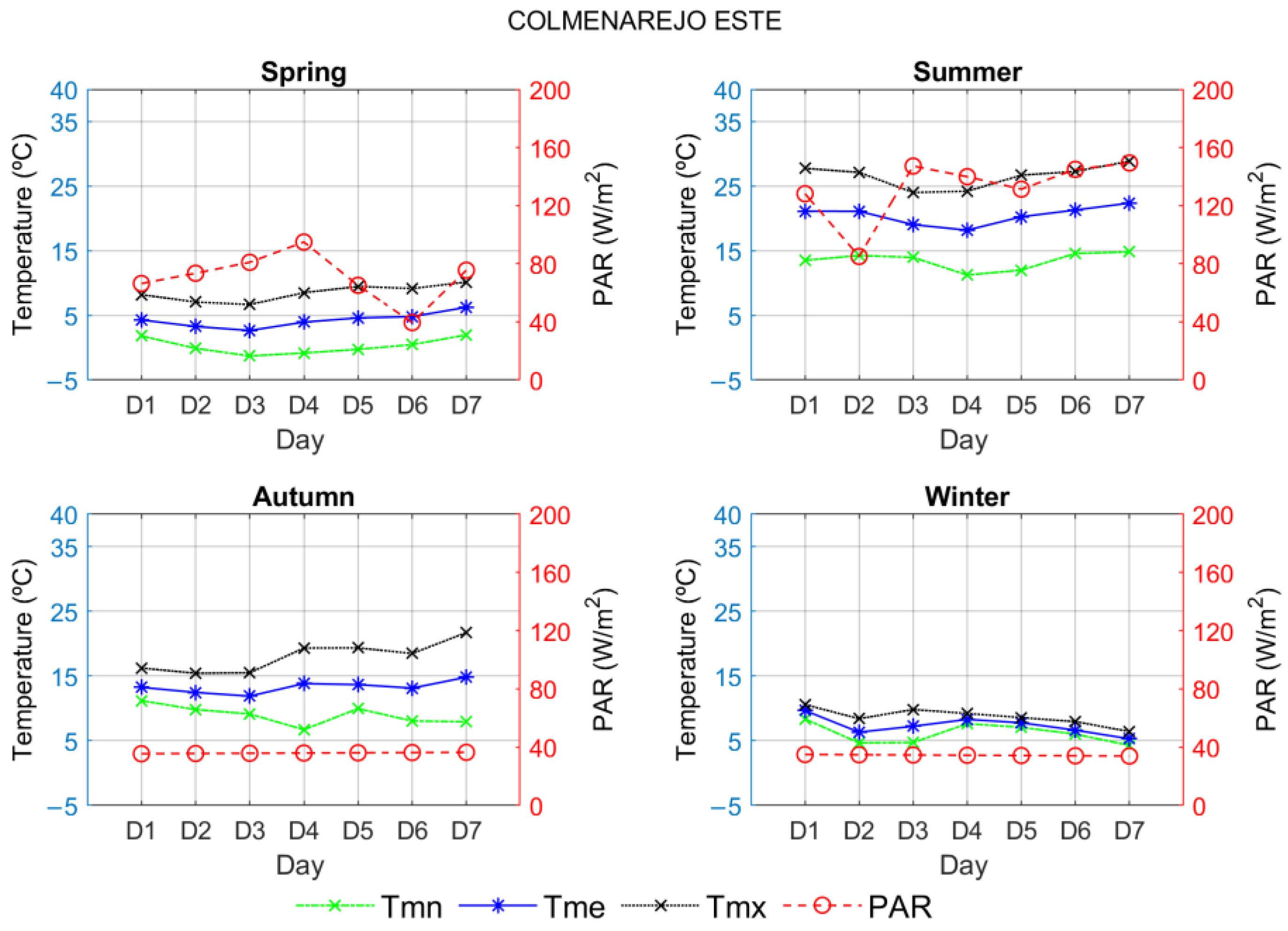
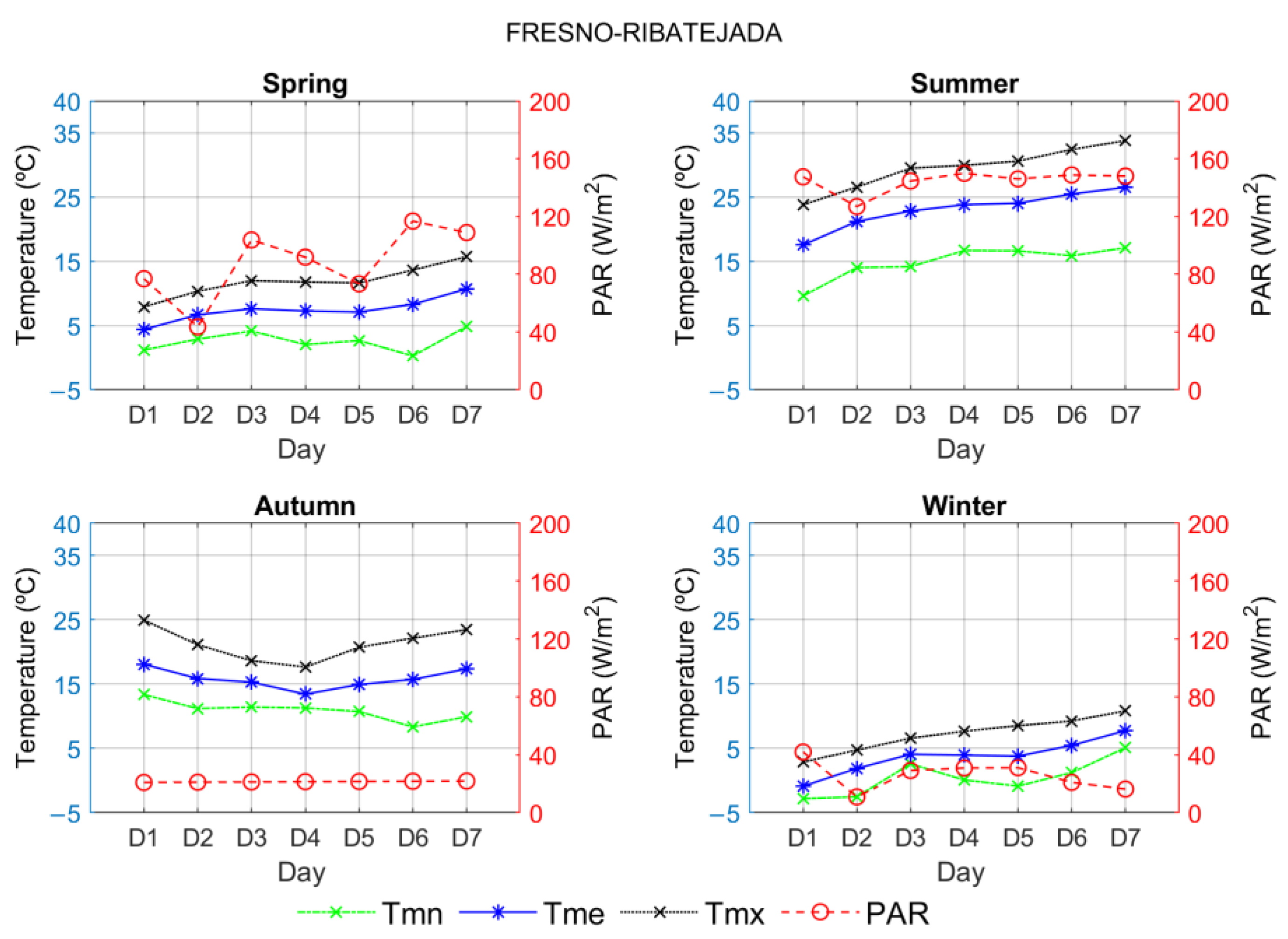
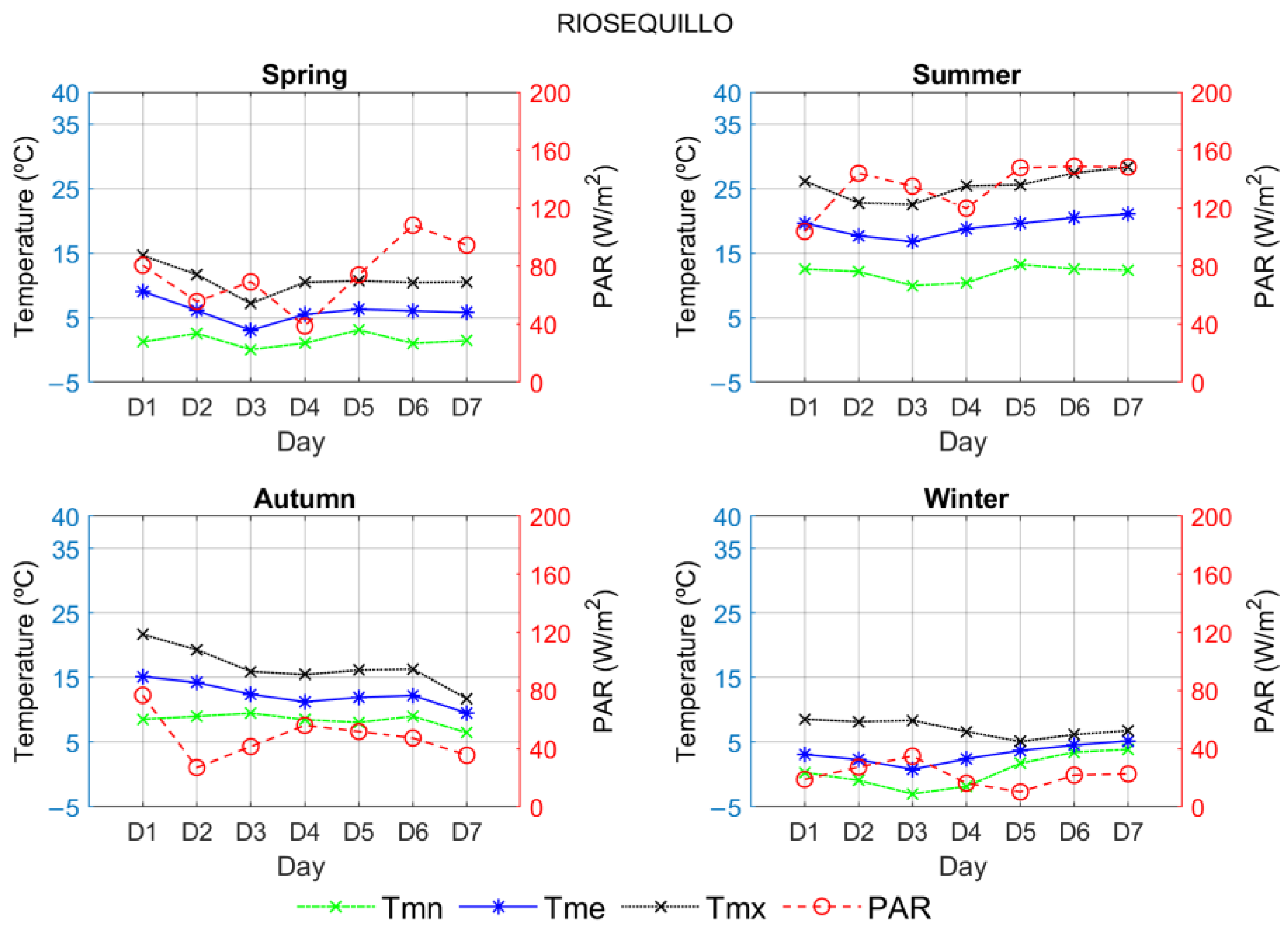
Biomass production and WWT are affected by uncontrollable meteorological parameters that vary throughout the cultivation period. Among these parameters, the temperature and solar irradiance between 400 and 700 nm (PAR) [36] are indispensable for microalgae growth [37,38,39,40,41]. The work carried out in [37] shows that the observed reduction in the mean daily PAR radiation entering the greenhouse affects the plant metabolism. The same effect is observed when the temperature stress is applied to the crop [42].

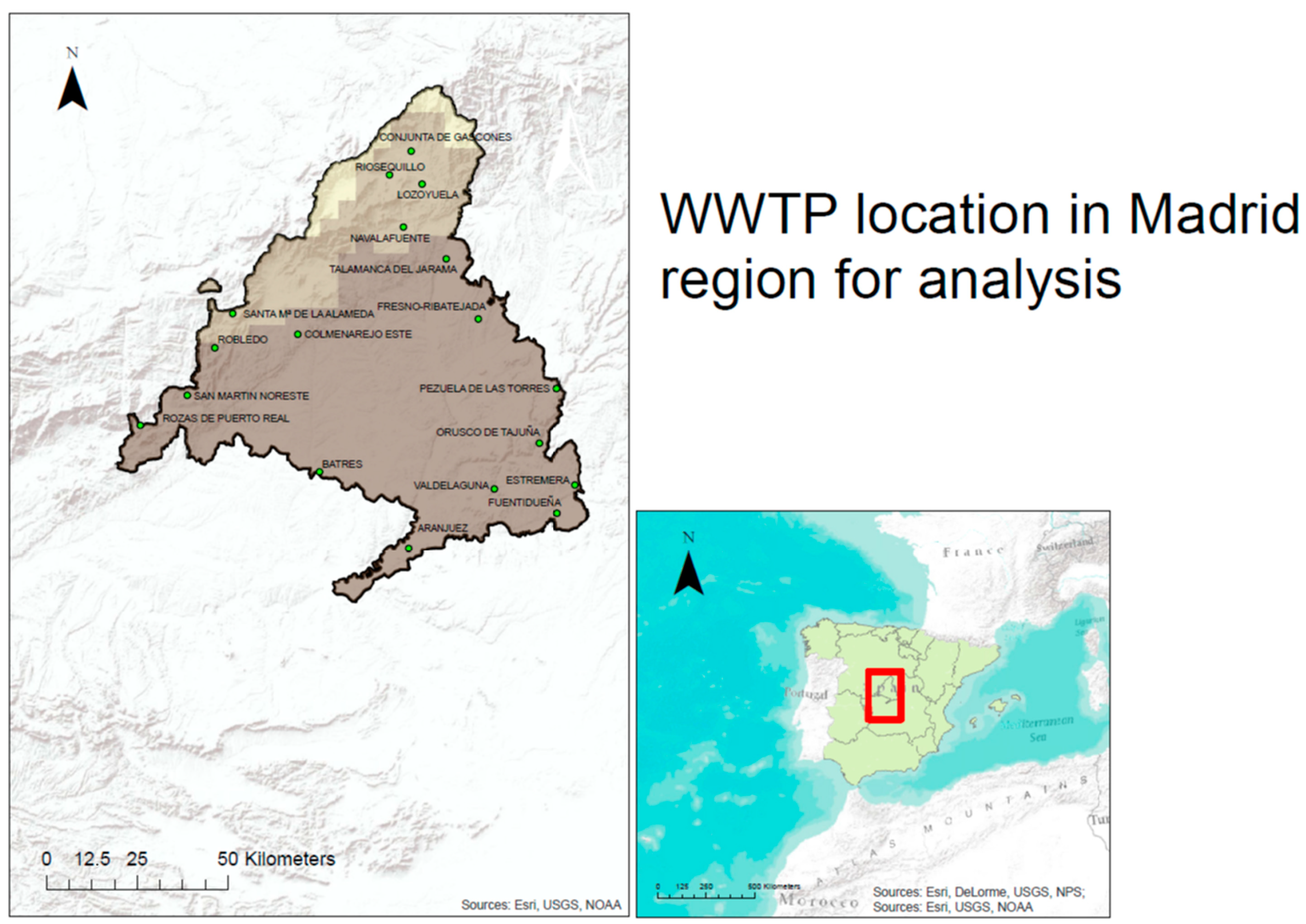
Therefore, due to the short hydraulic retention time for microalgae development, a TMS per meteorological season is studied using the data for the Madrid region. The four TMWs to be generated, one for each meteorological season, are based on the PAR and temperature in 18 wastewater treatment plants (WWTP) that already exist in the Madrid region, as shown in Figure 1.

Due to the availability of simultaneous PAR and temperature data in these locations of WWTPs, a 15-year set of PAR and daily mean, maximum, and minimum air temperature values was used. PAR has been obtained from Kato bands, provided by the spectral resolved irradiance (SRI) of the Satellite Application Facility on Climate Monitoring (CM-SAF), which belongs to the European Organization for the Exploitation of Meteorological Satellites (EUMETSAT) [43]. The daily mean temperature was obtained from the European Center for Medium-Range Weather Forecasts (ECMWF) [44]. The period used in the present study was 1991 to 2005, with a spatial resolution of 0.125° × 0.125°.

These four parameters are then grouped into a matrix in which two additional columns, the temperature range and the solar day length, were added by calculations. The latter is used to take into account the photoperiod; that is, the number of solar hours during which microalgae are exposed to PAR and the maximum possible duration of the solar day [45].

Madrid is almost located in the center of the Iberian Peninsula (between 41.15° N and 39.88° N latitude and between 3.05° W and 4.57° W longitude) on the Central Plateau, and the altitude ranges from 476 to 2428 m and the average is 678 m above sea level, with a surface area of approximately 8000 km². The orography of the Madrid region is characterized by the presence of the Central Mountain Range in the north and west of the territory, while the remaining areas are the plains and the Tajo River Valley. The climate of the region is strongly influenced by its orography. Therefore, in the range and its surroundings, there is a mountain climate (Dsc according to the Köppen-Geiger classification) [46,47,48] and an oceanic-Mediterranean climate (Csb). On the other hand, there is a typical Mediterranean climate (Csa) in the plains and a semi-arid climate (BSk) in the southern areas and around the Tajo River Valley. This variation in climate could be estimated by generating TMS that reflect this variability in the growth of microalgae.

2.3. Applying the TMS Methodology

The growth and productivity of microalgae is challenged by multiple cultivation parameters, such as pH, nutrients, light, temperature, agitation, cultivation medium, etc. For our case, only physical parameters, solar irradiance (PAR and solar day length), and temperatures are considered in this scientific approach to study the effects of both parameters on microalgae activity.

Therefore, the existence of values of these parameters at which the culture is at its optimum level or not leads us to consider different weight factor cases for temperature and irradiance. For this purpose, an approach based on TMY methodologies is used to determine the importance of the meteorological parameters in the growth period of microalgae. Moreover, as these two cultivation parameters change significantly between two meteorological seasons, a seasonal approach is adopted. Each season is examined separately, following a multistage process.

Firstly, the whole set of data available (15 years in our case study) has been distributed in the four seasons (E_{w = 1, 2, 3, 4}): 1 = spring (March–May), 2 = summer (June–August), 3 = autumn (September–November), and 4 = winter (December–February) in that order. These seasons are based on the annual temperature cycle and not on the astronomical seasons, so there is a clear transition between them. For each location, there is a time series corresponding to 14 seasons (A_{y = 1, 2, …, 14}) for each of these four weather seasons. Thereafter, a period of time is identified as follows E_wA_y. For example, E₁A₄ represents the spring season (E₁) of 1994 (A₄), which is the first spring of the 14 spring seasons that we have between March 1991 and May 2004. Additionally, E₄A₁₄ represents the winter season that starts in December 2004 and ends in February 2005.

Since it is intended to characterize one week (S_p) over a season, and a week is a set of seven consecutive days (not necessarily beginning on Monday and ending on Sunday), the proposal is based on an increase in the available data so that the number of candidate weeks over the study period increases. In addition, for a given season, the weeks are constituted in such a way that there is a discontinuity when passing from one year to the next. In other words, in a sequence (week in our case), we cannot have days that come from two different years. This procedure will generate p weeks from the q available days per meteorological season (d_q) in the following way:

$$\begin{array}{c}{\mathrm{E}}_{\mathrm{w}}{\mathrm{A}}_{\mathrm{y}}=\left\{{\mathrm{d}}_1,{\mathrm{d}}_2,\dots ,{\mathrm{d}}_{\mathrm{q}}\right\}\\ \begin{array}{ccc}{\mathrm{S}}_1=\left\{{\mathrm{d}}_1,{\mathrm{d}}_2,\dots ,{\mathrm{d}}_7\right\},& {\mathrm{S}}_2=\left\{{\mathrm{d}}_2,{\mathrm{d}}_3,\dots ,{\mathrm{d}}_8\right\},& \begin{array}{cc}\dots & {\mathrm{S}}_{\mathrm{p}}=\left\{{\mathrm{d}}_{\mathrm{q}-6},{\mathrm{d}}_{\mathrm{q}-5},\dots ,{\mathrm{d}}_{\mathrm{q}}\right\}\end{array}\end{array}\end{array}$$

where p = q − 6. This represents an increase of nearly 700% in the number of candidate weeks for a season in each year (season) of the time series. The data obtained (all 7-day packages) represent, for example, all candidate weeks for all spring seasons between March 1991 and May 2004. The same has been done for the other meteorological seasons. Therefore, this procedure generated a good number (q) of candidate weeks for each of these four weather seasons: 1204 for spring, 1204 for summer, 1190 for autumn, and finally, 1184 for winter.

Thereafter, for the entire dataset corresponding to each season and for each week (of each season), a Cumulative Distribution Function (CDF), Equation (1), is determined for each one of the six selected meteorological parameters: PAR, solar day length, mean, maximum, minimum, and temperature range.

The CDF of each meteorological parameter (x) was calculated by classifying the dataset into equally sized intervals, often called lags, because the size of the long-term data is different from that of short-term data. This is why it is interesting to use lags to perform Equation (2). Thereafter, the number n of observations is equal to the number of lags (n). Finally, the observations are arranged in ascending order x₁, x₂, …, x_n. The CDF of each observation is given by a monotonically increasing step function defined by:

$$\mathrm{C}\mathrm{D}\mathrm{F}(\mathrm{x})=\{\begin{array}{c}\begin{array}{cc}\begin{array}{ccc}\begin{array}{cc}0& \begin{array}{cc}& \end{array}\end{array}& \mathrm{for}& \mathrm{x}<{\mathrm{x}}_1\end{array}& \end{array}\\ \begin{array}{ccc}\begin{array}{c}\frac{\left(\mathrm{k}-0.5\right)}{\mathrm{n}}\end{array}& \mathrm{for}& {\mathrm{x}}_{\mathrm{k}}\le \mathrm{x}\le {\mathrm{x}}_{\mathrm{k}+1}\end{array}\\ \begin{array}{cc}\begin{array}{ccc}\begin{array}{cc}1& \begin{array}{cc}& \end{array}\end{array}& \mathrm{for}& \mathrm{x}>{\mathrm{x}}_{\mathrm{n}}\end{array}& \end{array}\end{array}$$

(1)

where k is the order number from 1 to n − 1.

Then, the FS statistics of each sequence (in our case one week) for each given parameter (x) are obtained from the following Equation (2). In other words, the FS statistics for the candidate week are obtained by calculating the differences between the CDF (defined in Equation (1)) for this week (short-term) with the CDF for all the weeks contained in the corresponding weather season (long term) for each parameter and location.

$$\begin{array}{c}\mathrm{F}\mathrm{S}=\frac{1}{\mathrm{n}}{\displaystyle \sum _{\mathrm{i}=1}^{\mathrm{n}}{\mathsf{\delta }}_{\mathbf{i}}}\\ {\mathsf{\delta }}_{\mathrm{i}}=\left|\mathrm{C}\mathrm{D}{\mathrm{F}}_{\mathrm{l}\mathrm{t}}({\mathrm{x}}_{\mathrm{i}})-\mathrm{C}\mathrm{D}{\mathrm{F}}_{\mathrm{s}\mathrm{t}}({\mathrm{x}}_{\mathrm{i}})\right|\end{array}$$

(2)

with CDF_lt and CDF_st as the long-term and short-term CDF of parameter x.

A weighted sum (WS) of the FS statistics corresponding to each parameter (FS_j) of each week is calculated by applying a weight factor (wf_j), where m is the number of meteorological parameters:

$$\mathrm{W}\mathrm{S}={\displaystyle \sum _{\mathrm{j}=1}^{\mathrm{m}}\mathrm{w}{\mathrm{f}}_{\mathrm{j}}}·\mathrm{F}{\mathrm{S}}_{\mathrm{j}}$$

(3)

The weighting factor chosen will depend on the importance that each parameter has on the growth of microalgae and must comply with:

$${\displaystyle \sum _{\mathrm{j}=1}^{\mathrm{m}}\mathrm{w}{\mathrm{f}}_{\mathrm{j}}}=1$$

(4)

Following the process, the ‘best’ candidate weeks (applying different options of wfs) are chosen according to a proportion determining the impact on the growth of microalgae. Thus, the proposal is to analyze the influence that these wfs have on the ranking of candidate weeks for a TMW.

Indeed, the generation of TMYs was done using different climate parameters and different weighting factors [10,17,25,45,49,50]. All these proposals are essentially similar; the main differences are the climate parameters to be included (type and quantity) and their corresponding weighting factors.

The studied parameters: temperature (mean, maximum, minimum, and range); PAR; and solar day length play an important role in the development of a TMS. However, in our case study, they do not have the same impact on microalgae productivity. Therefore, some meteorological parameters may be more important than others. The most influential parameters receive the highest weighting factor (wf_j), which is considered representative of their impact on microalgae growth.

In

Table 1. Weighting factor (wf) options to obtain the weighted sum.

Parameters	wf_1	wf_2	wf_3	wf_4	wf_5	wf_6	wf_7	wf_8	wf_9
Tmx	0.10	0.05	0.05	0.10	0.05	0.05	0.05	0.05	0.10
Tmn	0.10	0.05	0.05	0.10	0.05	0.05	0.05	0.05	0.10
Tme	0.30	0.40	0.30	0.25	0.25	0.45	0.40	0.40	0.20
Trg	-	-	-	0.05	0.05	0.05	0.05	0.05	0.10
PAR	0.30	0.20	0.30	0.25	0.30	0.20	0.30	0.15	0.20
Nsol	0.20	0.30	0.30	0.25	0.30	0.20	0.15	0.30	0.30

, nine scenarios with different wfs are proposed to test different options of wfs. This will allow us to check the robustness of the methodology. The idea is to give equal importance to the temperature parameters—maximum (Tmx), minimum (Tmn), mean (Tme), range (Trg), solar irradiance, PAR, and solar day length (Nsol).

Finally, the most representative sequence—week, in our case—among the five best-candidate weeks is obtained by determining the frequency of repetition of the candidate weeks, taking into account their persistence according to the different lags and wfs. Furthermore, the final decision on the choice of the TMW is also affected by its position in the particular season period. This position is validated by calculating the difference in Nsol between the day in the middle of the weather season and the fourth day of the candidate week, Equation (5). This was done to avoid extreme values for a season that could compromise expected results. The difference in Nsol is defined as follows:

$$\Delta \mathrm{N}\mathrm{s}\mathrm{o}{\mathrm{l}}_{\mathrm{q}}^{\mathrm{w}}=\left|\mathrm{N}\mathrm{s}\mathrm{o}{\mathrm{l}}_{\mathrm{q}/2}^{\mathrm{w}}-\mathrm{N}\mathrm{s}\mathrm{o}{\mathrm{l}}_4^{\mathrm{w}}\right|$$

(5)

where $\mathrm{N}\mathrm{s}\mathrm{o}{\mathrm{l}}_{\mathrm{q}/2}^{\mathrm{w}}$ represents the Nsol of the fourth day of the week in the middle of the considered weather season (w = 1, 2, 3, and 4 for spring, summer, autumn, and winter). $\mathrm{N}\mathrm{s}\mathrm{o}{\mathrm{l}}_4^{\mathrm{w}}$ is Nsol of the fourth day of the given candidate week.

3. Results and Discussion

Although microalgae growth is affected by several physicochemical parameters, such as temperature, light, pH, salinity, nutrients, and others, the results and discussion presented in this paper are limited to the input of solar energy and temperature.

The five weeks with the lowest WS values were selected for each WWTP. The selected TMW has a notable persistence and a low difference in $\Delta \mathrm{N}\mathrm{s}\mathrm{o}{\mathrm{l}}_{\mathrm{q}}^{\mathrm{w}}$. The persistence of a week corresponds to the number of times it appears in the selection for different weighting factors and lag. By broadening the final choice criteria with more weighting factors and lags, a sequence of new candidate weeks emerges that might be different from their predecessors. In some cases, the same weeks are repeated but in a different order. Finally, the selected TMW is supposed to present the long-term characteristic properties of the meteorological data. The same process is adopted for each of the four meteorological seasons for each of the 18 WWPTs.

To facilitate the presentation of the results, only the details of the long-term and weekly statistics are presented in the following tables. The rest of the results are given in Appendix A.

Table 2. Long-term daily statistics in Colmenarejo Este.

Spring
	Temperature (°C)				Solar Irradiance (W/m2)
	Tmx	Tmn	Tme	Trg	PAR	Nsol
Mean	16.25	5.40	10.84	10.85	91.26	13.05
Median	16.05	5.11	10.45	10.98	92.99	13.13
Av. Std. Des	4.81	3.41	3.97	3.43	28.99	1.04
Summer
	Temperature (°C)				Solar irradiance(W/m2)
	Tmx	Tmn	Tme	Trg	PAR	Nsol
Mean	28.46	15.54	22.29	12.91	126.57	14.35
Median	29.21	16.00	22.88	13.30	130.40	14.58
Av. Std. Des	4.41	3.26	3.80	2.48	20.52	0.57
Autumn
	Temperature (°C)				Solar irradiance(W/m2)
	Tmx	Tmn	Tme	Trg	PAR	Nsol
Mean	17.27	8.00	12.39	9.27	61.25	10.91
Median	16.71	8.06	12.06	9.42	58.03	10.85
Av. Std. Des	6.10	4.54	5.18	3.35	26.51	1.02
Winter
	Temperature (°C)				Solar irradiance(W/m2)
	Tmx	Tmn	Tme	Trg	PAR	Nsol
Mean	8.61	0.50	4.10	8.11	39.68	9.63
Median	8.54	0.12	4.12	8.00	41.24	9.39
Av. Std. Des	2.91	2.98	2.65	3.07	16.35	0.55

shows the seasonal quarterly statistics for the Colmenarejo Este location during the period 1991 to 2005. It includes the mean and median of each of the six parameters for the different seasons, as well as the standard deviation, which provides information about the average dispersion of each of these. A standard deviation between 2.48 and 6.10 is observed for the temperature parameters. The PAR has a high standard deviation with values distributed over a range between 16.35 and 28.99, while the Nsol is about one for spring and autumn and less than one for summer and winter. The daily or seasonal variability of these growth parameters significantly affects the production of microalgae. Taking into account seasonal variations, it can be shown that winter has unfavorable meteorological conditions with less light, very low temperatures, and an inadequate photoperiod for microalgae growth. Summer offers the appropriate ranges of values to maximize productivity, while spring and autumn are unfavorable for microalgae metabolism. Extreme variations in these parameters can be observed throughout the year and can have inhibiting effects on microalgae.

Due to the large number of weeks to evaluate nine wf options (Table 1), the WS of the FS statistics for the different parameters are not presented in tabular form in this article.

Table 3. The candidate weeks of the spring season in Colmenarejo Este presented for different sets of weighting factors and lag sizes.

	wf	wf_1	wf_2	wf_3	wf_4	wf_5	wf_6	wf_7	wf_8	wf_9
lags
lags = 10		1082	1082	642	641	642	235	642	235	235
		641	235	235	235	235	641	235	641	641
		642	641	641	642	641	642	641	642	642
		235	642	1082	1082	1081	1081	1081	1082	378
		507	1081	1081	378	507	1082	1082	1081	1082
lags = 20		642	642	642	642	642	642	642	642	642
		1082	1081	1081	641	641	235	641	235	235
		641	1082	641	235	235	1081	235	641	641
		496	641	235	1082	1081	641	1081	1081	1082
		235	235	507	496	507	1082	1082	1082	864
lags = 30		642	642	642	642	642	642	642	642	642
		1082	1082	507	235	235	1081	235	235	235
		496	1081	1081	641	641	235	1081	1081	641
		641	641	641	1082	507	641	641	939	378
		507	496	1082	496	1081	1082	507	641	1082

shows the results obtained for the spring season in the Colmenarejo Este location: each cell shows the number of the candidate week corresponding to a set of weight factors (column) and a number of lags (rows). For each pair of ‘weighting factors set and lag size’, we present the five best candidates ordered from top to bottom according to the minimum WS value. In the case of Colmenarejo Este, the total number of weeks analyzed is 1204, so that—for example—week number 235 represents the sequence of seven days that begins on 2 May 1993.

The TMW for each season and each of the 18 locations are given in

Table A2. First day of the Typical Meteorological Week of each season for each of the EDAR stations.

Site	Season	Year	Month	Day	Site	Season	Year	Month	Day
ARANJUEZ	Spring	1994	03	20	ORUSCO DE TAJUÑA	Spring	2003	04	20
	Summer	1997	06	20		Summer	1995	06	19
	Autumn	1993	11	06		Autumn	1996	11	20
	Winter	1996	12	18		Winter	1992	12	18
BATRES	Spring	1993	05	02	PEZUELA DE LAS TORRES	Spring	1993	05	02
	Summer	1991	06	19		Summer	1997	06	15
	Autumn	1996	10	19		Autumn	1996	09	08
	Winter	1996	12	14		Winter	1994	12	16
COLMENAREJO ESTE	Spring	1998	04	09	RIOSEQUILLO	Spring	2002	04	09
	Summer	1994	06	16		Summer	1994	06	17
	Autumn	1996	09	20		Autumn	1994	10	13
	Winter	1996	12	18		Winter	2000	12	18
CONJUNTA DE GASCONES	Spring	2003	04	19	ROBLEDO	Spring	1995	04	03
	Summer	1991	06	19		Summer	1991	06	19
	Autumn	1996	11	21		Autumn	1996	09	20
	Winter	1995	12	14		Winter	1996	12	15
ESTREMERA	Spring	1993	03	17	ROZAS DE PUERTO REAL	Spring	1996	03	27
	Summer	1994	06	19		Summer	1998	06	19
	Autumn	1996	11	20		Autumn	2001	09	27
	Winter	1996	12	16		Winter	1996	12	15
FRESNO-RIBATEJADA	Spring	2002	04	11	SAN MARTIN NORESTE	Spring	2001	05	18
	Summer	1991	06	19		Summer	2000	06	15
	Autumn	1996	09	08		Autumn	1999	10	11
	Winter	1995	12	14		Winter	1996	12	15
FUENTIDUEÑA	Spring	2003	04	20	SANTA Mª DE LA ALAMEDA	Spring	1998	05	20
	Summer	1995	06	19		Summer	1994	06	16
	Autumn	1998	09	21		Autumn	1996	09	20
	Winter	1996	12	16		Winter	1996	12	15
LOZOYUELA	Spring	2002	04	09	TALAMANCA DEL JARAMA	Spring	2003	04	19
	Summer	1997	06	20		Summer	1997	06	20
	Autumn	1996	09	20		Autumn	1996	09	20
	Winter	2000	12	18		Winter	1994	12	16
NAVALAFUENTE	Spring	2003	04	19	VALDELAGUNA	Spring	1993	05	02
	Summer	1997	06	20		Summer	1997	06	20
	Autumn	1994	10	13		Autumn	1998	09	21
	Winter	1996	12	16		Winter	1992	12	18

. In this table, only the first day of the selected week is given. Although the years of the selected weeks are not identical, it can be observed that there is a slight difference in the periods (months and days) of the year for the sites studied. This difference could be due to the variations of the average temperatures that decrease with the latitude. However, the variations of the PAR between locations are very small and are due to the small differences in latitude from one point to another. The latter may have little influence on the expected results, especially since the RAP difference is very little between locations. Other factors that also play a very important role in the generation of weeks are the wfs assigned to the variables and the lag number (Table 3). If we focus on one column (wf value) from Table 3, we can see that almost the same weeks come back with different positions when we change the lag number. Likewise, when we look at a lag number, the trend of results also changes each time we change the distribution of wfs and in the same sense as previously mentioned, hence the interest in choosing several wf options that can compensate for the lack of information of the meteorological parameter with the most important impact on the growth of microalgae.

Table 4. Candidate weeks in the Colmenarejo Este location in the spring season.

Number of Week	Frequency	Year	Month	Day	$\mathbf{N}\mathbf{s}\mathbf{o}{\mathbf{l}}_4^{\mathbf{w}}$	$\mathbf{\Delta }\mathbf{N}\mathbf{s}\mathbf{o}{\mathbf{l}}_{\mathbf{q}}^{\mathbf{w}}$
235	24	1993	5	2	13.91	0.78
378	3	1995	4	3	12.64	0.49
496	5	1996	5	5	14.05	0.92
507	8	1996	5	16	14.41	1.28
641	27	1998	4	8	12.91	0.22
642	27	1998	4	9	12.96	0.18
864	1	2001	3	4	11.31	1.82
939	1	2001	5	18	14.44	1.31
1081	18	2003	4	18	13.35	0.21
1082	21	2003	4	19	13.39	0.26

shows the information for all generated candidate weeks for the spring season in Colmenarejo Este that are represented in Table 3. In Table 4, the number of repetitions of these generated candidate weeks is also shown, which are represented by their order number in the sequence of 1204 spring weeks. Once a candidate week is selected, its sequence number identifies the start of the week by giving the corresponding year, month, and day.

The Nsol of the fourth day $\left(\mathrm{N}\mathrm{s}\mathrm{o}{\mathrm{l}}_4^{\mathrm{w}}\right)$ of each of these candidate weeks is also given in this table, as well as the absolute value of the difference $\left(\Delta \mathrm{N}\mathrm{s}\mathrm{o}{\mathrm{l}}_{\mathrm{q}}^{\mathrm{w}}\right)$ between the Nsol of the fourth day of the week in the middle of the season $\left(\mathrm{N}\mathrm{s}\mathrm{o}{\mathrm{l}}_{\mathrm{q}/2}^{\mathrm{w}}\right)$ and the Nsol of the candidate week $\left(\mathrm{N}\mathrm{s}\mathrm{o}{\mathrm{l}}_4^{\mathrm{w}}\right)$. This difference allows us to appreciate the position of the week in relation to the extremities of that season. As mentioned above, this avoids having a typical week with weather conditions closer to the earlier or later season. Therefore, the selected TMW has the highest frequency of occurrence. In the case event that this frequency of occurrence is equal, then the typical weather week would be the one with the lowest value of $\left(\Delta \mathrm{N}\mathrm{s}\mathrm{o}{\mathrm{l}}_{\mathrm{q}}^{\mathrm{w}}\right)$. For example, the Nsol on the fourth day of the week in the middle of the spring season in the Colmenarejo Este location is 12.96 h.

According to the different weeks presented in Table 4, the frequency of occurrence in week 641 is the same as in week 642. This coincidence in the number of occurrences can be explained by the fact that these two weeks differ by one day: one starts on 8 April 1998 and the other on 9 April 1998. Therefore, the final choice of the representative week of spring meteorological conditions in Colmenarejo Este is given by the week with the lowest $\left(\Delta \mathrm{N}\mathrm{s}\mathrm{o}{\mathrm{l}}_{\mathrm{q}}^{\mathrm{w}}\right)$ value. In the case of Colmenarejo Este, week 642 is the typical week that represents the spring weather conditions for the period 1991 to 2005.

The Madrid region is not very large, and consequently, a small difference of the order of magnitude for both PAR and temperature is observed in a given season when moving from one locality to another (Figure 2, Figure A1, Figure A2 and Figure A3). This can also be seen in Table 2 and

Table A1. Long-term data statistics for four sites.

FRESNO-RIBATEJADA
	Spring			Summer			Autumn			Winter
	Mean	Median	Std. Dev.	Mean	Median	Std. Dev.	Mean	Median	Std. Dev.	Mean	Median	Std. Dev.
Tmx	16.36	16.20	4.83	28.55	29.41	4.38	17.34	16.75	6.09	8.73	8.62	2.91
Tmn	5.55	5.25	3.43	15.67	16.13	3.29	8.11	8.22	4.54	0.68	0.27	2.97
Tme	10.95	10.52	4.00	22.41	23.01	3.78	12.46	12.17	5.16	4.25	4.29	2.63
Trg	10.81	10.94	3.45	12.88	13.30	2.46	9.24	9.45	3.37	8.05	7.96	3.10
PAR	93.53	94.58	28.07	126.61	130.02	19.44	62.46	59.39	26.16	40.31	41.47	16.22
NSol	13.05	13.13	1.04	14.35	14.59	0.58	10.91	10.85	1.02	9.62	9.39	0.55
RIOSEQUILLO
	Spring			Summer			Autumn			Winter
	Mean	Median	Std. Dev.	Mean	Median	Std. Dev.	Mean	Median	Std. Dev.	Mean	Median	Std. Dev.
Tmx	15.21	14.99	4.76	27.06	27.75	4.44	16.23	15.69	6.02	7.80	7.73	2.95
Tmn	4.22	4.05	3.39	13.84	14.18	3.22	6.83	6.99	4.40	−0.24	−0.57	2.99
Tme	9.69	9.37	3.92	20.72	21.27	3.76	11.24	10.95	5.00	3.31	3.31	2.65
Trg	10.99	11.00	3.59	13.22	13.61	2.71	9.39	9.44	3.56	8.03	7.93	3.12
PAR	85.56	87.74	30.37	121.60	127.06	23.67	56.75	53.00	26.28	36.83	38.15	16.25
NSol	13.07	13.15	1.05	14.38	14.62	0.58	10.89	10.83	1.04	9.59	9.36	0.56
VALDELAGUNA
	Spring			Summer			Autumn			Winter
	Mean	Median	Std. Dev.	Mean	Median	Std. Dev.	Mean	Median	Std. Dev.	Mean	Median	Std. Dev.
Tmx	17.36	17.14	4.93	29.82	30.67	4.35	18.24	17.70	6.16	9.49	9.36	2.90
Tmn	6.49	6.14	3.51	17.10	17.63	3.35	9.00	9.01	4.73	1.25	0.92	3.06
Tme	11.92	11.43	4.09	23.76	24.35	3.80	13.37	12.99	5.32	4.92	5.00	2.66
Trg	10.87	11.18	3.44	12.71	13.07	2.31	9.24	9.51	3.28	8.24	8.27	3.18
PAR	94.36	95.49	27.66	127.23	130.60	18.73	63.75	60.96	25.94	41.55	42.45	15.88
NSol	13.04	13.12	1.02	14.32	14.55	0.57	10.92	10.86	1.01	9.66	9.43	0.55

(Appendix A), in which the statistics of long-term meteorological data are given for four locations.

The daily mean values of the TMW parameters for each season were obtained, and the variability of some parameters was plotted, which is illustrated in Figure 2, showing the daily variation of the mean values of PAR and temperature indices for the different seasons. Figure 2, Figure A1, Figure A2 and Figure A3 indicate that, for both meteorological parameters, there is inter-seasonal variability. The highest PAR and temperature values are observed during summer, and the lowest values are observed during winter. On the one hand, thermal oscillation is greater between summer and winter. Since Madrid is located in the central peninsular area, a possible explanation may come from the disappearance of the moderating effect of the sea, which decreases as one moves away from the coast. Furthermore, Figure 2, Figure A1, Figure A2 and Figure A3 show that the temperature range is narrower in winter. The spring and autumn seasons have approximately similar average daily temperatures. However, the daily average PAR is lower in autumn compared to spring, and its variability is sometimes similar to that of winter in certain localities. This can be explained by the predominance of cloudy and probably rainy skies at this time of year. In fact, cloudiness reduces insolation by obstructing solar radiation.

4. Conclusions

In this work, a methodology for the generation of TMS for the simulation of photosynthetic organism growth and productivity for WWT or agriculture is proposed. The selection of potential sequences according to the growth period of the organism is performed by resampling the available meteorological data, which, in our case study, increases the number of candidate sequences by 700%.

Prior knowledge of the impact of meteorological factors would allow the optimization of crop productivity, rational use of water, and evaluate the appropriate period during the year for WWT in a HRAP systems with microalgae. It is relevant to take into account the long-term variability of physical parameters among the seasons to develop sustainable systems. The advantage of TMS data is that they are suitable to overcome computational power limitations when multiple simulations are needed to have an overview of the biological system behavior as a function of local climatic conditions.

The TMS approach has allowed to generate a typical sequence called TMW intended to simulate the growth of microalgal biomass for biofuel production or sustainable wastewater treatment in a HRAP. For the generation of the TMW in our case study, once the most relevant climatic parameters were identified, a detailed exam of the different weight factors for each of the variables considered was performed to ensure the robustness of the methodology.

References

1. Domínguez, A.; Martínez-Romero, A.; Leite, K.N.; Tarjuelo, J.M.; de Juan, J.A.; López-Urrea, R. Combination of Typical Meteorological Year with Regulated Deficit Irrigation to Improve the Profitability of Garlic Growing in Central Spain. Agric. Water Manag. 2013, 130, 154–167. [Google Scholar] [CrossRef]
2. Garfí, M.; Flores, L.; Ferrer, I. Life Cycle Assessment of Wastewater Treatment Systems for Small Communities: Activated Sludge, Constructed Wetlands and High Rate Algal Ponds. J. Clean. Prod. 2017, 161, 211–219. [Google Scholar] [CrossRef]
3. López-Sánchez, A.; Silva-Gálvez, A.L.; Aguilar-Juárez, Ó.; Senés-Guerrero, C.; Orozco-Nunnelly, D.A.; Carrillo-Nieves, D.; Gradilla-Hernández, M.S. Microalgae-Based Livestock Wastewater Treatment (MbWT) as a Circular Bioeconomy Approach: Enhancement of Biomass Productivity, Pollutant Removal and High-Value Compound Production. J. Environ. Manag. 2022, 308, 114612. [Google Scholar] [CrossRef] [PubMed]
4. Acién, F.G.; Gómez-Serrano, C.; Morales-Amaral, M.M.; Fernández-Sevilla, J.M.; Molina-Grima, E. Water Treatment Using Microalgae: How Realistic a Contribution Might It Be to Significant Urban Wastewater Treatment. Appl. Microbiol. Biotechnol. 2016, 100, 9013–9022. [Google Scholar] [CrossRef] [PubMed]
5. Robles, Á.; Capson-Tojo, G.; Galès, A.; Ruano, M.V.; Sialve, B.; Ferrer, J.; Steyer, J.P. Microalgae-Bacteria Consortia in High-Rate Ponds for Treating Urban Wastewater: Elucidating the Key State Indicators under Dynamic Conditions. J. Environ. Manag. 2020, 261, 110244. [Google Scholar] [CrossRef]
6. Arcila, J.S.; Buitrón, G. Influence of Solar Irradiance Levels on the Formation of Microalgae-Bacteria Aggregates for Municipal Wastewater Treatment. Algal Res. 2017, 27, 190–197. [Google Scholar] [CrossRef]
7. Iasimone, F.; Panico, A.; De Felice, V.; Fantasma, F.; Iorizzi, M.; Pirozzi, F. Effect of Light Intensity and Nutrients Supply on Microalgae Cultivated in Urban Wastewater: Biomass Production, Lipids Accumulation and Settleability Characteristics. J. Environ. Manag. 2018, 223, 1078–1085. [Google Scholar] [CrossRef]
8. Hall, I.J.; Prairie, R.R.; Anderson, H.E.; Boes, E.C. Generation of Typical Meteorological Years for 26 SOLMET Stations; Sandia Laboratories: Albuquerque, NM, USA, 1978.
9. Leite, K.N.; Martínez-Romero, A.; Tarjuelo, J.M.; Domínguez, A. Distribution of Limited Irrigation Water Based on Optimized Regulated Deficit Irrigation and Typical Metheorological Year Concepts. Agric. Water Manag. 2015, 148, 164–176. [Google Scholar] [CrossRef]
10. Marion, W.; Urban, K. User’s Manual for TMY2s Radiation Data Base; National Renewable Energy Laboratory: Golden, CO, USA, 1995.
11. Fernández, M.D.; López, J.C.; Baeza, E.; Céspedes, A.; Meca, D.E.; Bailey, B. Generation and Evaluation of Typical Meteorological Year Datasets for Greenhouse and External Conditions on the Mediterranean Coast. Int. J. Biometeorol. 2015, 59, 1067–1081. [Google Scholar] [CrossRef]
12. Heinemann, P.H.; Walker, P.N. Effects of Greenhouse Surface Heating Water on Light Transmission. Trans. ASAE 1987, 30, 0215–0220. [Google Scholar] [CrossRef]
13. Marbis, J.M. CO2 Enrichment and Hot Water Heat in a Greenhouse as a Mean of Recovering Bioresources from Swine Waste; North Carolina State University: Raleigh, NC, USA, 2001. [Google Scholar]
14. Martínez-Romero, A.; Domínguez, A.; Landeras, G. Regulated Deficit Irrigation Strategies for Different Potato Cultivars under Continental Mediterranean-Atlantic Conditions. Agric. Water Manag. 2019, 216, 164–176. [Google Scholar] [CrossRef]
15. Shen, Q.H.; Jiang, J.W.; Chen, L.P.; Cheng, L.H.; Xu, X.H.; Chen, H.L. Effect of Carbon Source on Biomass Growth and Nutrients Removal of Scenedesmus Obliquus for Wastewater Advanced Treatment and Lipid Production. Bioresour. Technol. 2015, 190, 257–263. [Google Scholar] [CrossRef] [PubMed]
16. Baneshi, M.; Gonome, H.; Maruyama, S. Wide-Range Spectral Measurement of Radiative Properties of Commercial Greenhouse Covering Plastics and Their Impacts into the Energy Management in a Greenhouse. Energy 2020, 210, 118535. [Google Scholar] [CrossRef]
17. Kalogirou, S.A. Generation of Typical Meteorological Year (TMY-2) for Nicosia, Cyprus. Renew. Energy 2003, 28, 2317–2334. [Google Scholar] [CrossRef]
18. Pissimanis, D.; Karras, G.; Notaridou, V.; Gavra, K. The Generation of a “Typical Meteorological Year” for the City of Athens. Sol. Energy 1988, 40, 405–411. [Google Scholar] [CrossRef]
19. Skeiker, K. Generation of a Typical Meteorological Year for Damascus Zone Using the Filkenstein-Schafer Statistical Method. Energy Convers. Manag. 2004, 45, 99–112. [Google Scholar] [CrossRef]
20. Huld, T.; Paietta, E.; Zangheri, P.; Pascua, I.P. Assembling Typical Meteorological Year Data Sets for Building Energy Performance Using Reanalysis and Satellite-Based Data. Atmosphere 2018, 9, 53. [Google Scholar] [CrossRef] [Green Version]
21. Cebecauer, T.; Suri, M. Typical Meteorological Year Data: SolarGIS Approach. Energy Procedia 2015, 69, 1958–1969. [Google Scholar] [CrossRef] [Green Version]
22. Sun, J.; Li, Z.; Xiao, F. Analysis of Typical Meteorological Year Selection for Energy Simulation of Building with Daylight Utilization. Procedia Eng. 2017, 205, 3080–3087. [Google Scholar] [CrossRef]
23. Georgiou, G.; Eftekhari, M.; Eames, P.; Mourshed, M. A study of the effect of weighting indices for the development of TMY used for building simulation. In Proceedings of the BS2013: 13th Conference of International Building Performance Simulation Association, Chambéry, France, 26–28 August 2013; pp. 922–929. [Google Scholar]
24. Yang, L.; Wan, K.K.W.; Li, D.H.W.; Lam, J.C. A New Method to Develop Typical Weather Years in Different Climates for Building Energy Use Studies. Energy 2011, 36, 6121–6129. [Google Scholar] [CrossRef]
25. Chan, A.L.S.; Chow, T.T.; Fong, S.K.F.; Lin, J.Z. Generation of a Typical Meteorological Year for Hong Kong. Energy Convers. Manag. 2006, 47, 87–96. [Google Scholar] [CrossRef]
26. De Miguel, A.; Bilbao, J. Test Reference Year Generation from Meteorological and Simulated Solar Radiation Data. Sol. Energy 2005, 78, 695–703. [Google Scholar] [CrossRef]
27. Lund, H. Short Reference Years and Test Reference Years for EEC Countries; Technical Report. (Final Report, Contract ESF-029-DK, Report EUR 10208 EN.); Thermal Insulation Laboratory, Technical University of Denmark: Lyngby, Denmark, 1985. [Google Scholar]
28. Lund, H. The Design Reference Year. In Proceedings of the 91th Conference, International Building Performance Simulation Association, Nice, France, 20–22 August 1991; pp. 600–606. [Google Scholar]
29. Liem, S.H.; Van Paassen, A.H. Establishment of Short Reference Years for Calculation of Annual Solar Heat Gain or Energy Consumption in Residential and Commercial Buildings Part 1 and 2; Technical Report. (Report EUR 8912 EN); Commission of the European Communities: Luxembourg, 1984; pp. 1–38. [Google Scholar]
30. Zang, H.; Xu, Q.; Bian, H. Generation of Typical Solar Radiation Data for Different Climates of China. Energy 2012, 38, 236–248. [Google Scholar] [CrossRef]
31. Rodríguez, F.; Castro, A.; Marín, F.; Roldán, G.; Viteri Moya, F. Typical Meteorological Year Based on the Precipitation of Nanegalito and Pacto-Ecuador. Enfoque UTE 2019, 10, 197–204. [Google Scholar] [CrossRef] [Green Version]
32. Holzworth, D.P.; Huth, N.I.; de Voil, P.G.; Zurcher, E.J.; Herrmann, N.I.; McLean, G.; Chenu, K.; van Oosterom, E.J.; Snow, V.; Murphy, C.; et al. APSIM—Evolution towards a New Generation of Agricultural Systems Simulation. Environ. Model. Softw. 2014, 62, 327–350. [Google Scholar] [CrossRef]
33. Kephe, P.N.; Ayisi, K.K.; Petja, B.M. Challenges and Opportunities in Crop Simulation Modelling under Seasonal and Projected Climate Change Scenarios for Crop Production in South Africa. Agric. Food Secur. 2021, 10, 1–24. [Google Scholar] [CrossRef]
34. Huesemann, M.; Crowe, B.; Waller, P.; Chavis, A.; Hobbs, S.; Edmundson, S.; Wigmosta, M. A Validated Model to Predict Microalgae Growth in Outdoor Pond Cultures Subjected to Fluctuating Light Intensities and Water Temperatures. Algal Res. 2016, 13, 195–206. [Google Scholar] [CrossRef] [Green Version]
35. Wigmosta, M.S.; Coleman, A.M.; Skaggs, R.J.; Huesemann, M.H.; Lane, L.J. National Microalgae Biofuel Production Potential and Resource Demand. Water Res. 2011, 47, 1–13. [Google Scholar] [CrossRef]
36. Darvehei, P.; Bahri, P.A.; Moheimani, N.R. Modeling the Effect of Temperature on Microalgal Growth under Outdoor Conditions; Elsevier Masson SAS: Îledefrance, France, 2018; Volume 43, ISBN 9780444642356. [Google Scholar]
37. Baxevanou, C.; Fidaros, D.; Katsoulas, N.; Mekeridis, E.; Varlamis, C.; Zachariadis, A.; Logothetidis, S. Simulation of Radiation and Crop Activity in a Greenhouse Covered with Semitransparent Organic Photovoltaics. Appl. Sci. 2020, 10, 2550. [Google Scholar] [CrossRef] [Green Version]
38. García-Rodríguez, A.; García-Rodríguez, S.; Granados-López, D.; Díez-Mediavilla, M.; Alonso-Tristán, C. Extension of PAR Models under Local All-Sky Conditions to Different Climatic Zones. Appl. Sci. 2022, 5, 2372. [Google Scholar] [CrossRef]
39. Viruela, A.; Murgui, M.; Gómez-Gil, T.; Durán, F.; Robles, Á.; Ruano, M.V.; Ferrer, J.; Seco, A. Water Resource Recovery by Means of Microalgae Cultivation in Outdoor Photobioreactors Using the Effluent from an Anaerobic Membrane Bioreactor Fed with Pre-Treated Sewage. Bioresour. Technol. 2016, 218, 447–454. [Google Scholar] [CrossRef] [PubMed] [Green Version]
40. Breuer, G.; Lamers, P.P.; Martens, D.E.; Draaisma, R.B.; Wijffels, R.H. Effect of Light Intensity, PH, and Temperature on Triacylglycerol (TAG) Accumulation Induced by Nitrogen Starvation in Scenedesmus Obliquus. Bioresour. Technol. 2013, 143, 1–9. [Google Scholar] [CrossRef] [PubMed]
41. Cabello, J.; Toledo-Cervantes, A.; Sánchez, L.; Revah, S.; Morales, M. Effect of the Temperature, PH and Irradiance on the Photosynthetic Activity by Scenedesmus Obtusiusculus under Nitrogen Replete and Deplete Conditions. Bioresour. Technol. 2015, 181, 128–135. [Google Scholar] [CrossRef]
42. Jabri, H.A.; Taleb, A.; Touchard, R.; Saadaoui, I.; Goetz, V.; Pruvost, J. Cultivating Microalgae in Desert Conditions: Evaluation of the Effect of Light-temperature Summer Conditions on the Growth and Metabolism of Nannochloropsis Qu130. Appl. Sci. 2021, 11, 3799. [Google Scholar] [CrossRef]
43. Müller, R.; Pfeifroth, U.; Träger-Chatterjee, C.; Trentmann, J.; Cremer, R. Digging the METEOSAT Treasure-3 Decades of Solar Surface Radiation. Remote Sens. 2015, 7, 8067–8101. [Google Scholar] [CrossRef] [Green Version]
44. Hersbach, H.; Bell, B.; Berrisford, P.; Hirahara, S.; Horányi, A.; Muñoz-Sabater, J.; Nicolas, J.; Peubey, C.; Radu, R.; Schepers, D.; et al. The ERA5 Global Reanalysis. Q. J. R. Meteorol. Soc. 2020, 146, 1999–2049. [Google Scholar] [CrossRef]
45. Zhang, J.; Zhao, L.; Deng, S.; Xu, W.; Zhang, Y. A Critical Review of the Models Used to Estimate Solar Radiation. Renew. Sustain. Energy Rev. 2017, 70, 314–329. [Google Scholar] [CrossRef]
46. Beck, H.E.; Zimmermann, N.E.; McVicar, T.R.; Vergopolan, N.; Berg, A.; Wood, E.F. Present and Future Köppen-Geiger Climate Classification Maps at 1-Km Resolution. Sci. Data 2018, 5, 180214. [Google Scholar] [CrossRef] [Green Version]
47. Köppen, W.; Geiger, R. Das Geographische System Der Klimate; Gebrüder, B., Ed.; Mit 14 Textflguren: Berlin, Germany, 1936. [Google Scholar]
48. Peel, M.C.; Finlayson, B.L.; McMahon, T.A. Updated World Map of the Köppen-Geiger Climate Classification. Hydrol. Earth Syst. Sci. 2007, 11, 1633–1644. [Google Scholar] [CrossRef] [Green Version]
49. Skeiker, K. Comparison of Methodologies for TMY Generation Using 10 Years Data for Damascus, Syria. Energy Convers. Manag. 2007, 48, 2090–2102. [Google Scholar] [CrossRef]
50. Zarzalejo, L.F.; Téllez, F.M.; Heras, M. Creation of TMY for Southern Spanish Cities. In Proceedings of the International Symposium Passive Cooling of Buildings, Athens, Greece, 19–20 June 1995; pp. 61–73. [Google Scholar]
Figure 1. Location of WWTPs studied in the Madrid region.
Applsci 13 04826 g001
Figure 2. Daily variations of the daily mean values of temperature (mean, maximum, and minimum) and PAR for the selected TMWs for each season in Colmenarejo Este from 1991 to 2005.
Applsci 13 04826 g002