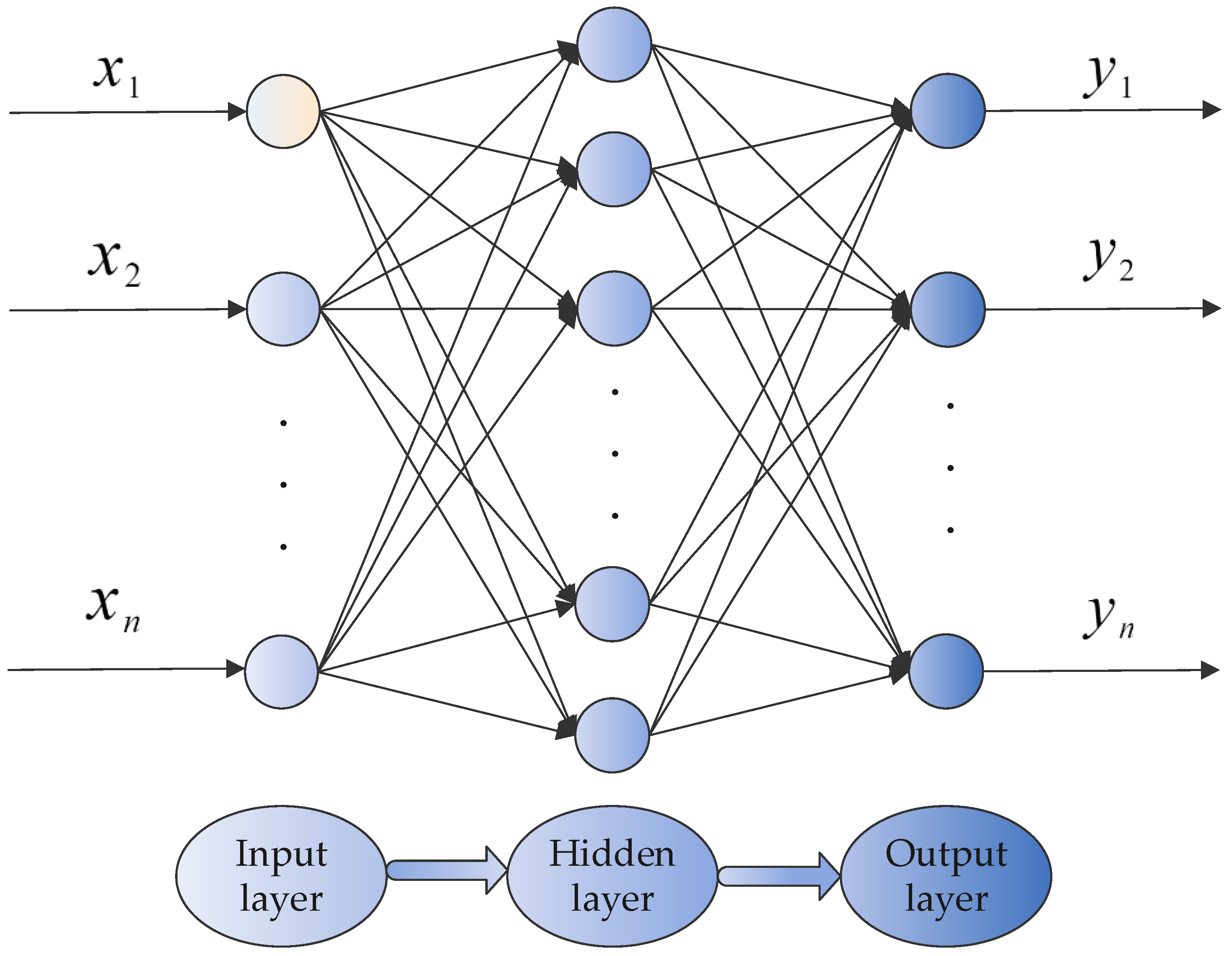
Figure 1.
Basic structure of a typical back propagation neural network (BPNN).
Figure 1.
Basic structure of a typical back propagation neural network (BPNN).
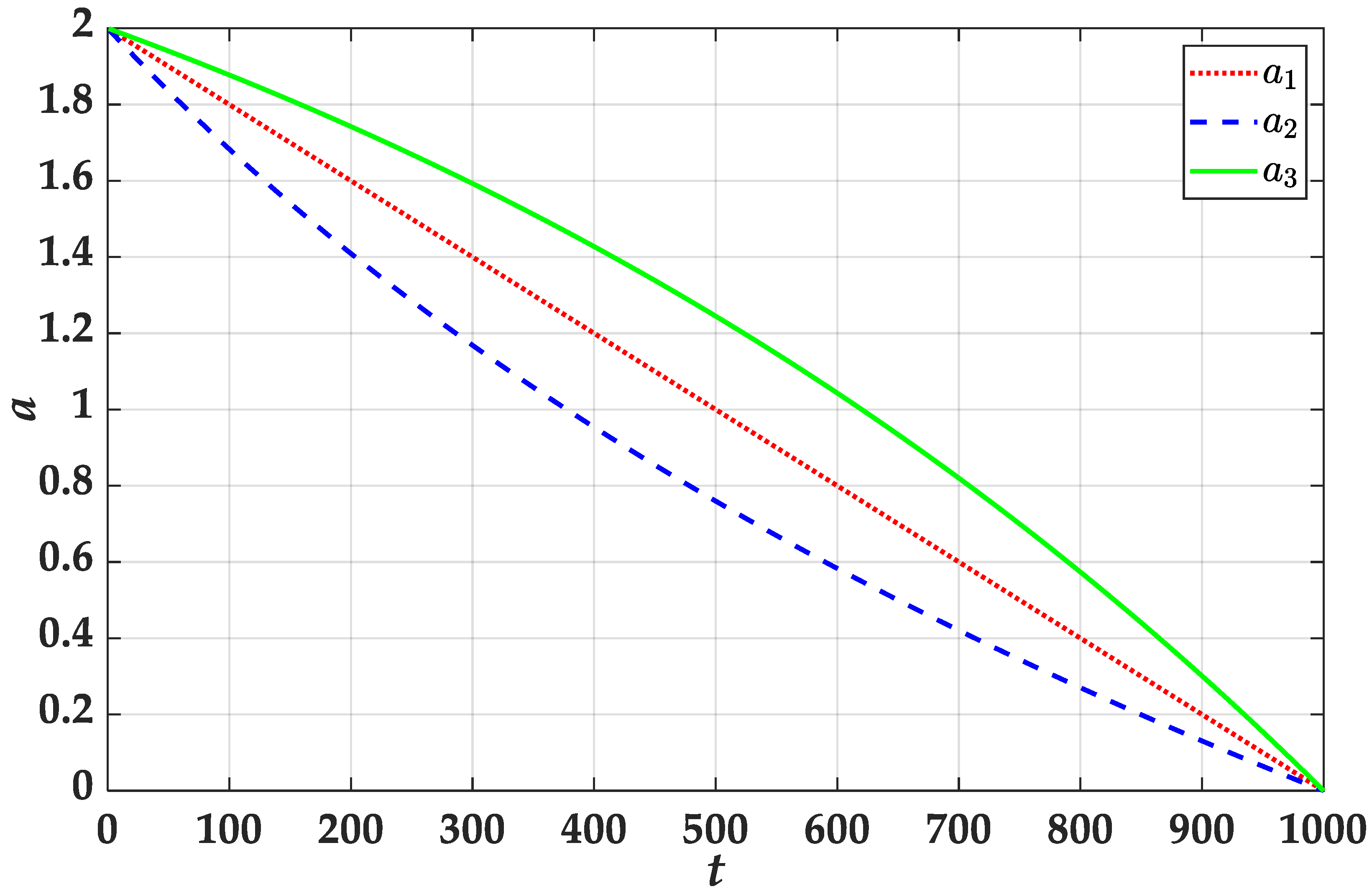
Figure 2.
The change of convergence factor.
Figure 2.
The change of convergence factor.
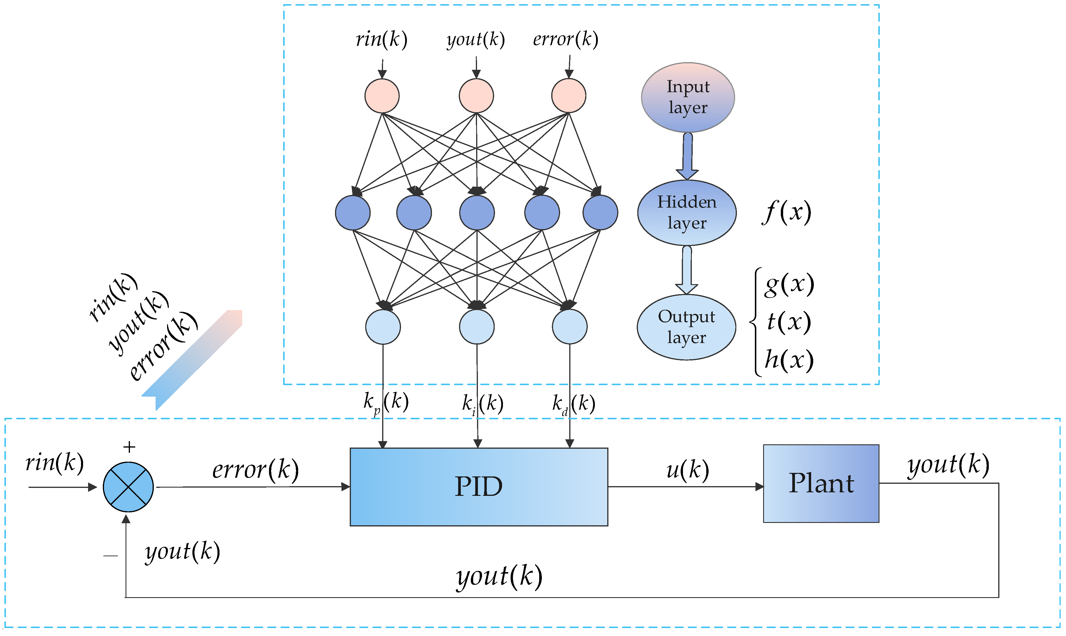
Figure 3.
The PID controller structure based on back propagation neural network.
Figure 3.
The PID controller structure based on back propagation neural network.
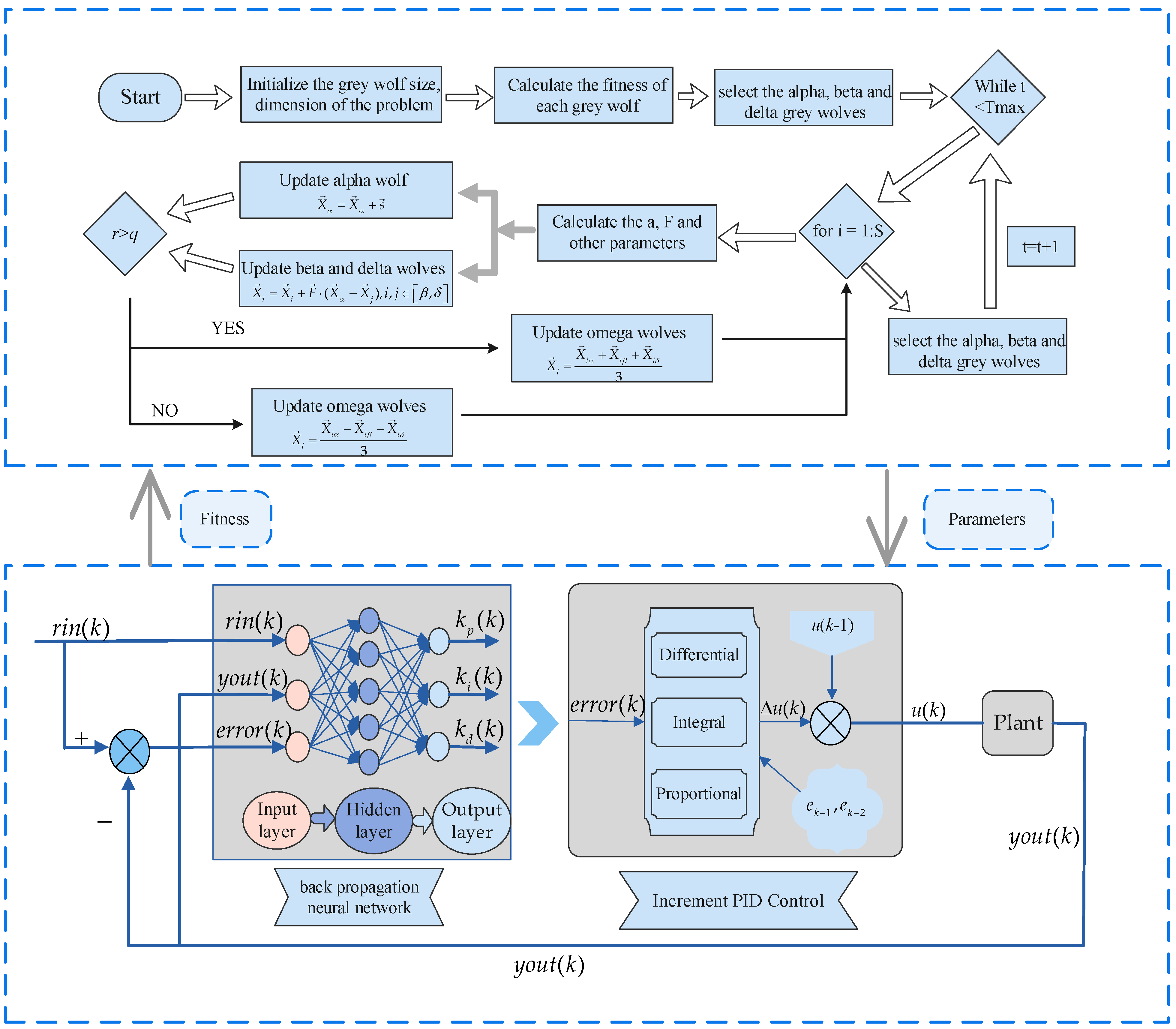
Figure 4.
The process of total algorithm.
Figure 4.
The process of total algorithm.
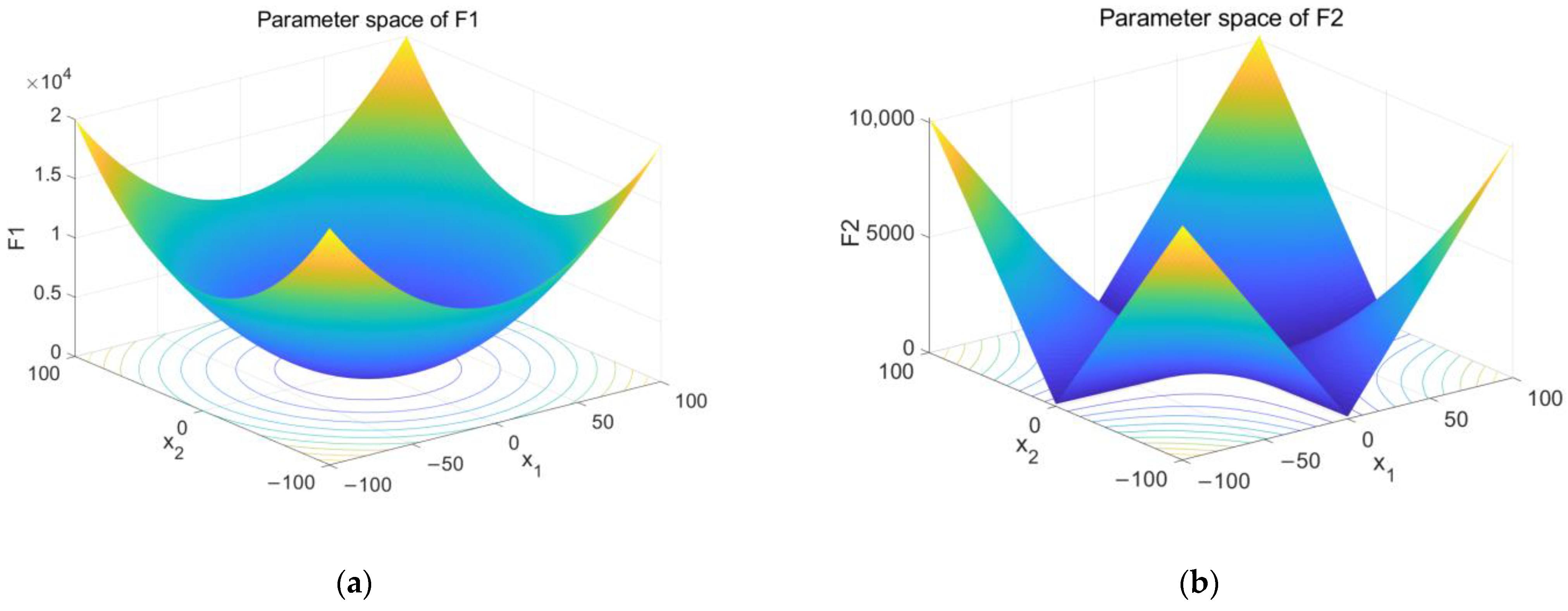
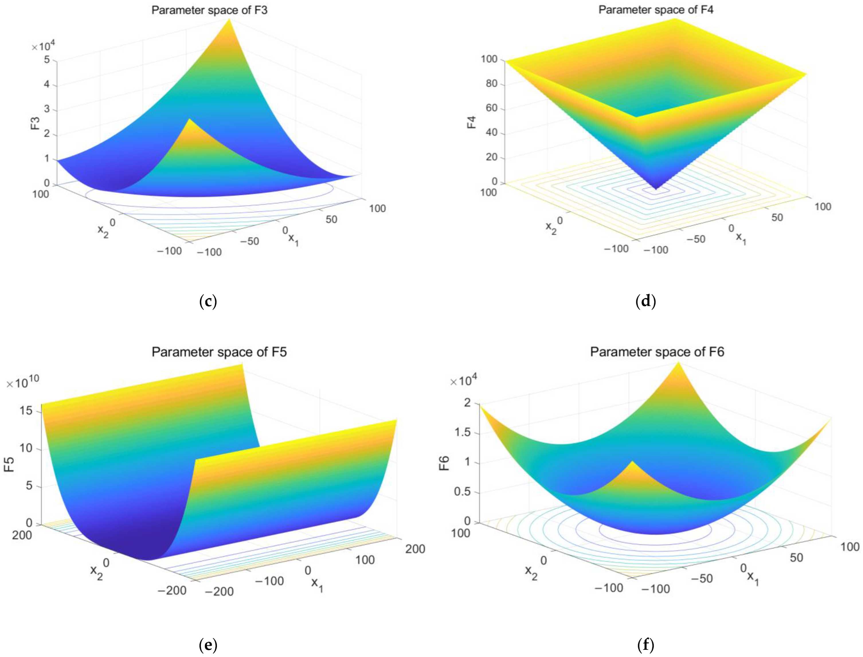
Figure 5.
The results of parameter space. (a) The parameter space of F1 and (b) the parameter space of F2 and (c) the parameter space of F3 and (d) the parameter space of F4 and (e) the parameter space of F5 and (f) the parameter space of F6.
Figure 5.
The results of parameter space. (a) The parameter space of F1 and (b) the parameter space of F2 and (c) the parameter space of F3 and (d) the parameter space of F4 and (e) the parameter space of F5 and (f) the parameter space of F6.
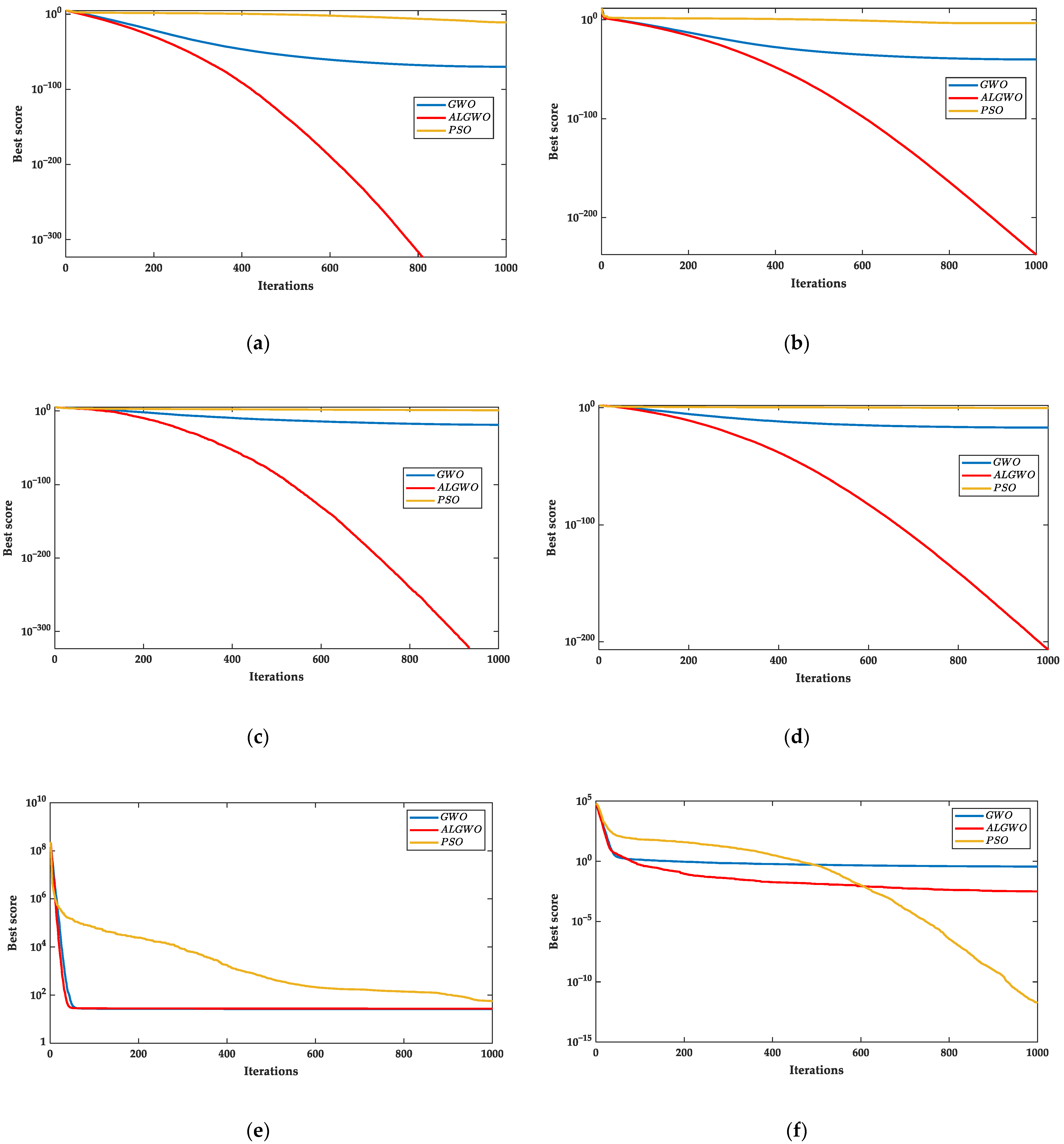
Figure 6.
The results of convergence curves. (a) The convergence curves of F1 and (b) the convergence curves of F2 and (c) the convergence curves of F3 and (d) the convergence curves of F4 and (e) the convergence curves of F5 and (f) the convergence curves of F6.
Figure 6.
The results of convergence curves. (a) The convergence curves of F1 and (b) the convergence curves of F2 and (c) the convergence curves of F3 and (d) the convergence curves of F4 and (e) the convergence curves of F5 and (f) the convergence curves of F6.
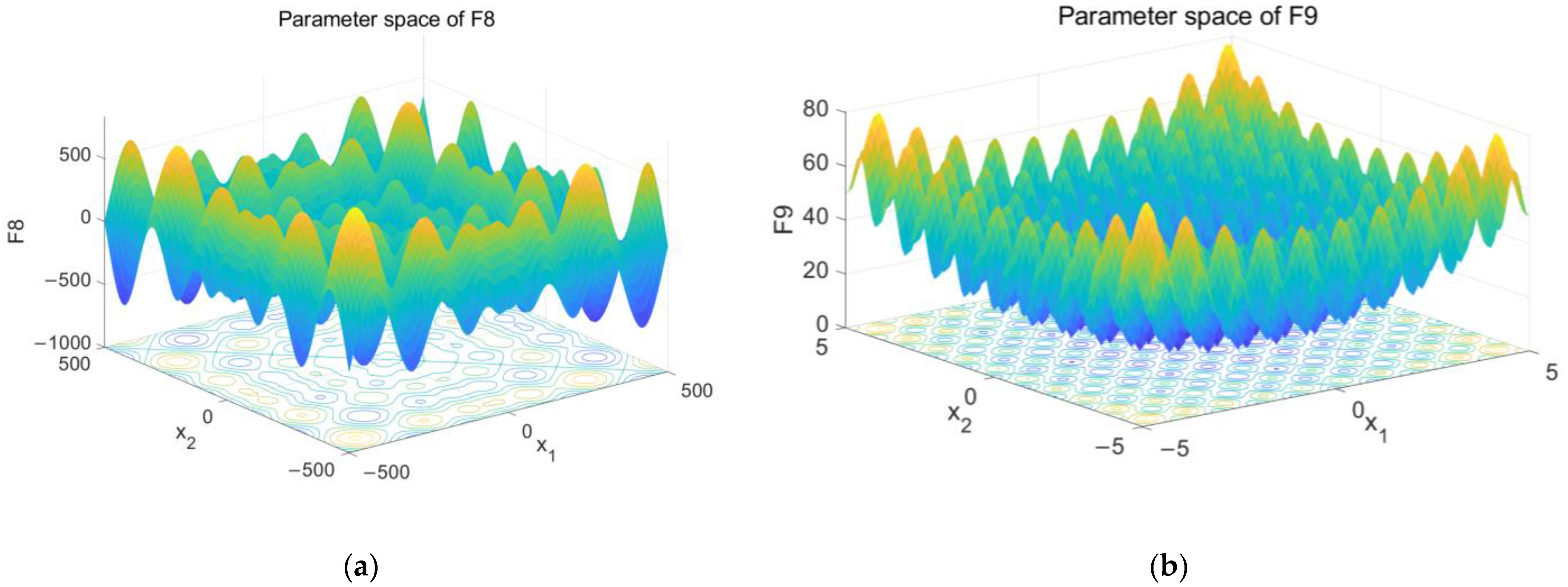
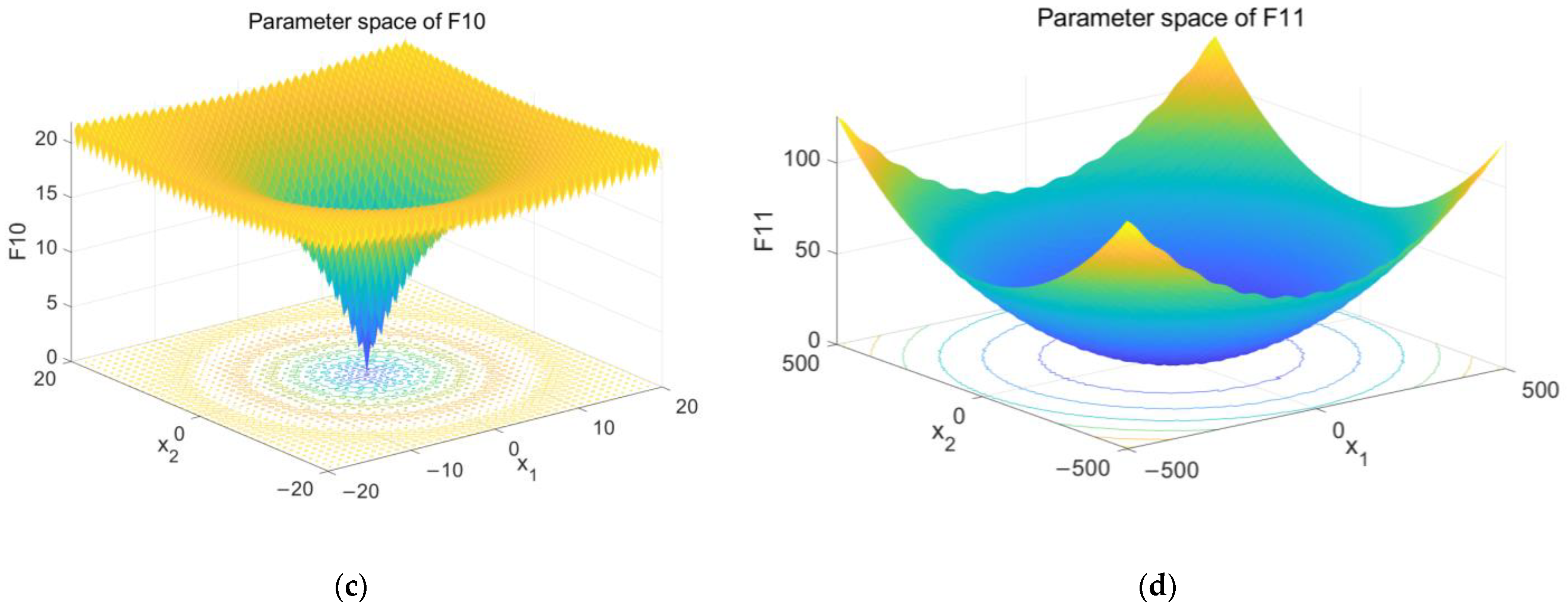
Figure 7.
The results of parameter space. (a) The parameter space of F8 and (b) the parameter space of F9 and (c) the parameter space of F10 and (d) the parameter space of F11.
Figure 7.
The results of parameter space. (a) The parameter space of F8 and (b) the parameter space of F9 and (c) the parameter space of F10 and (d) the parameter space of F11.
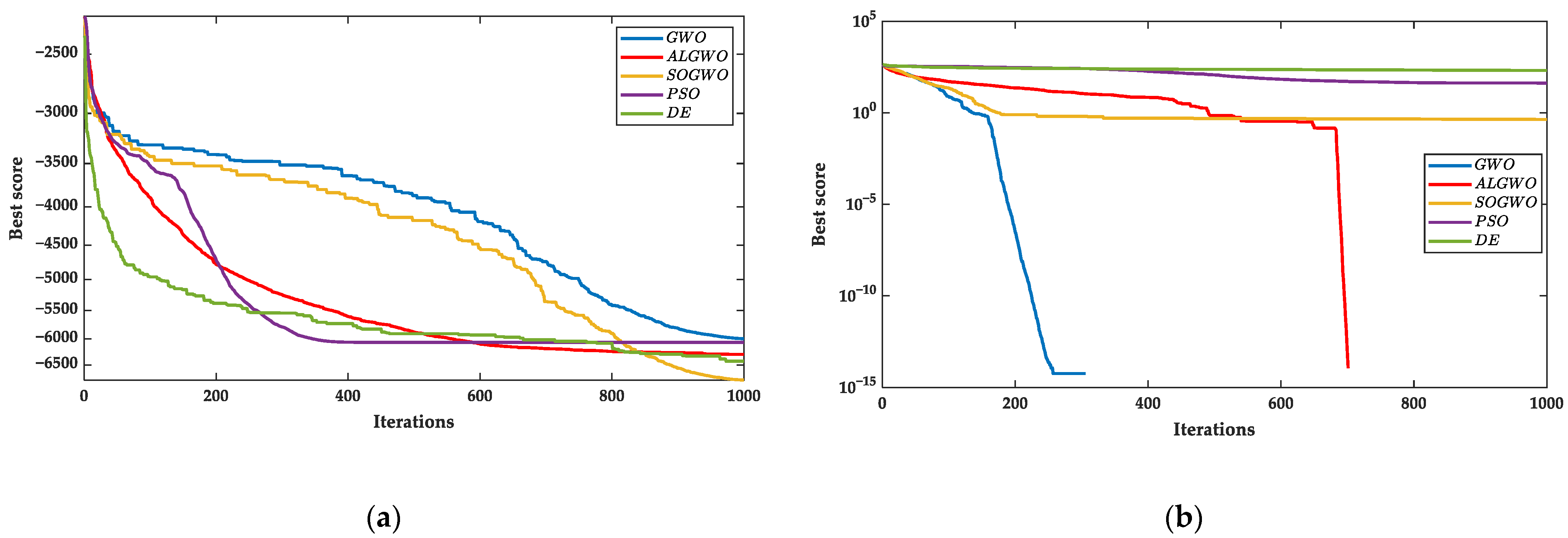
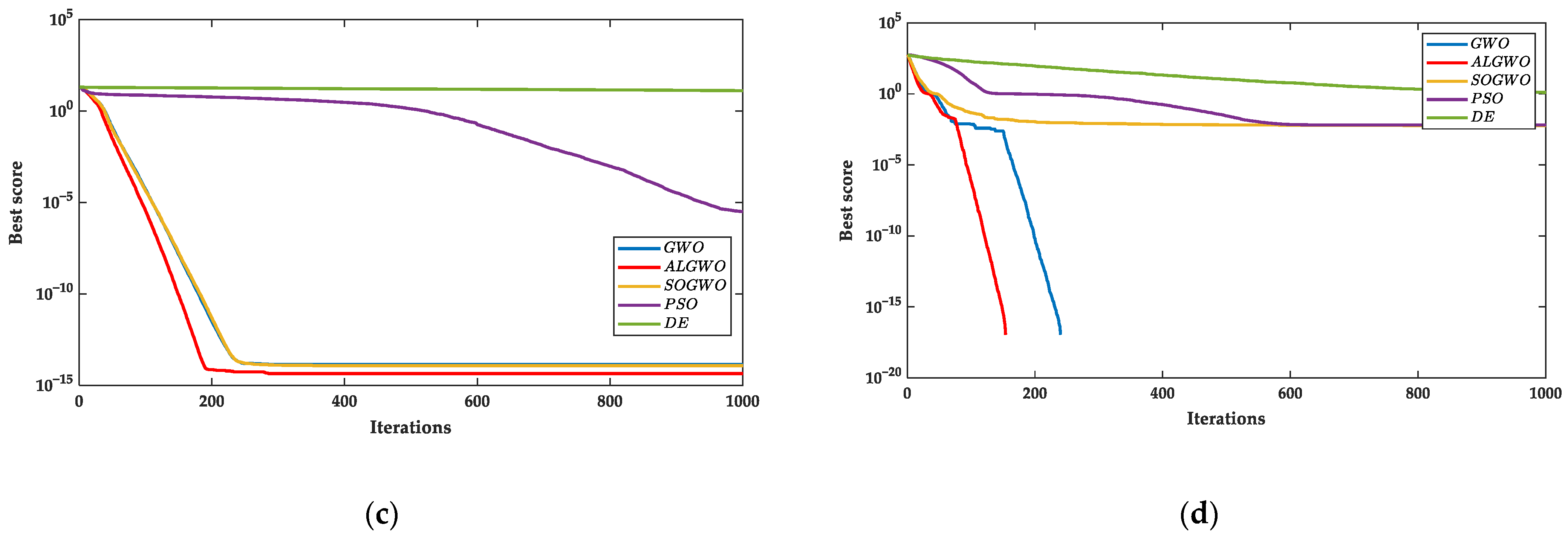
Figure 8.
The results of convergence curves. (a) The convergence curves of F8 and (b) the convergence curves of F9 and (c) the convergence curves of F10 and (d) the convergence curves of F11.
Figure 8.
The results of convergence curves. (a) The convergence curves of F8 and (b) the convergence curves of F9 and (c) the convergence curves of F10 and (d) the convergence curves of F11.
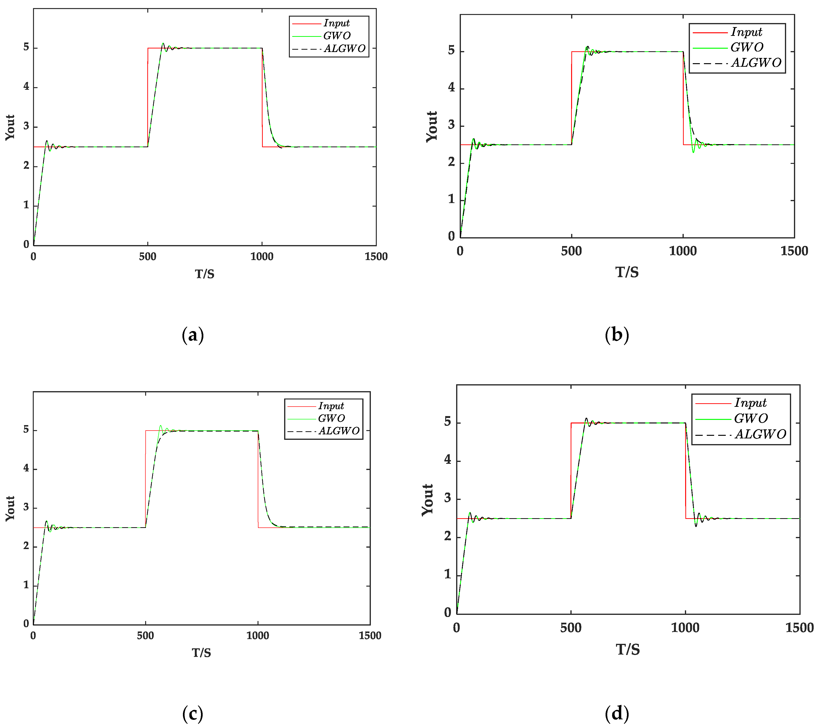
Figure 9.
The results of control effect. (a) The simulation results of BPNN-PID using g(x) and (b) simulation results of BPNN-PID using t(x) and (c) simulation results of BPNN-PID using h(x) and (d) simulation results of conventional PID.
Figure 9.
The results of control effect. (a) The simulation results of BPNN-PID using g(x) and (b) simulation results of BPNN-PID using t(x) and (c) simulation results of BPNN-PID using h(x) and (d) simulation results of conventional PID.
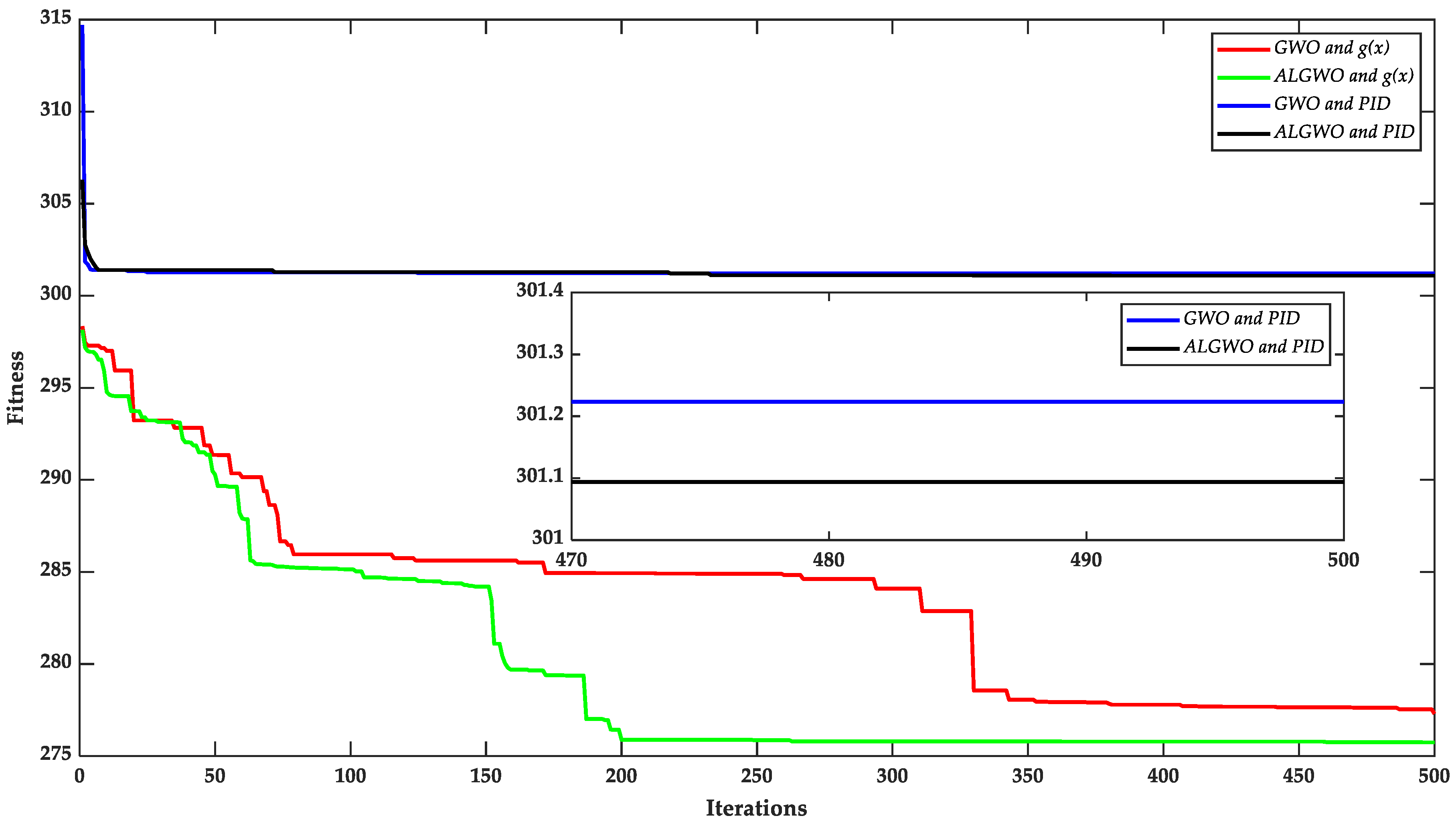
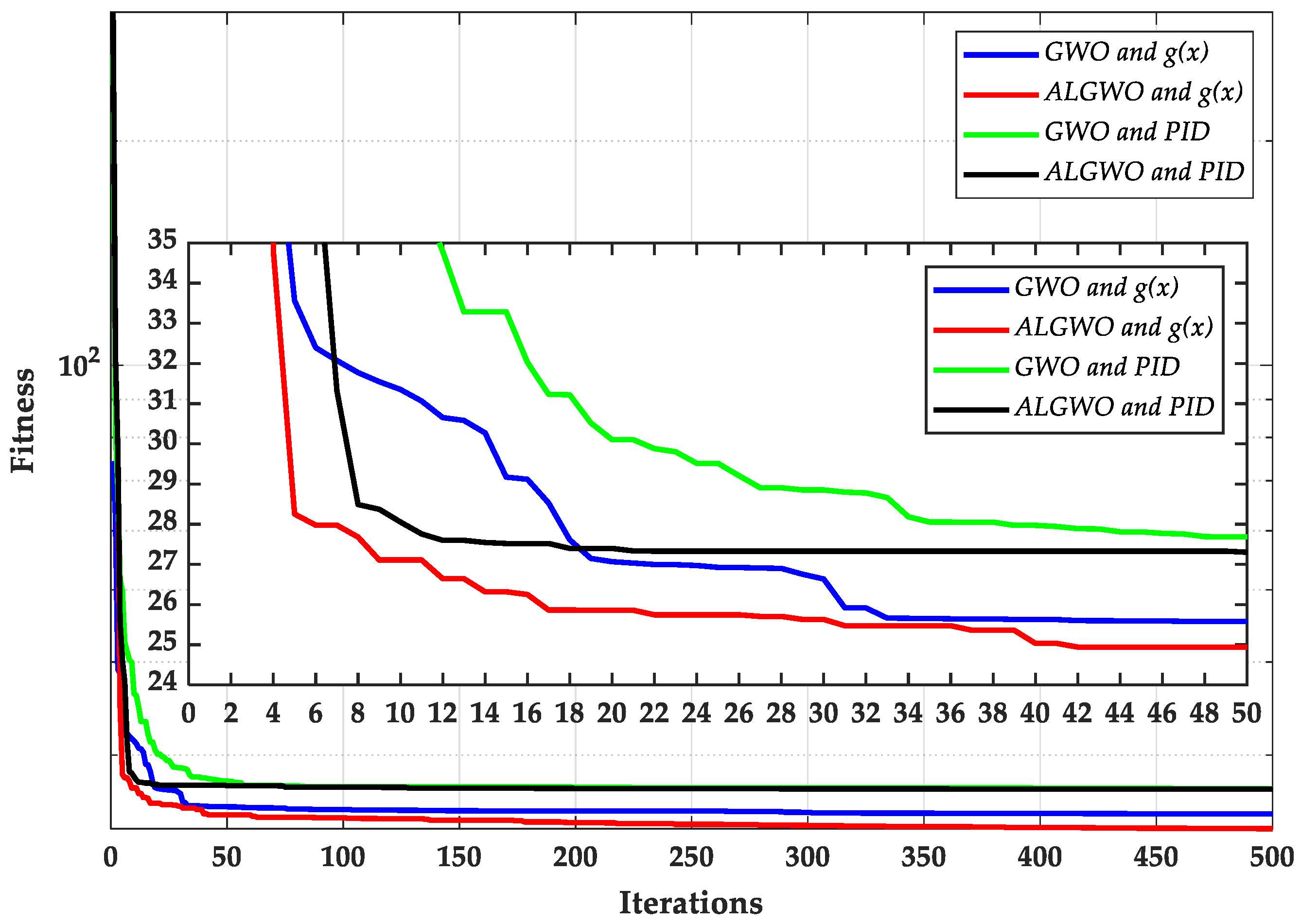
Figure 10.
The comparison results of algorithm optimization search on test system 3.
Figure 10.
The comparison results of algorithm optimization search on test system 3.
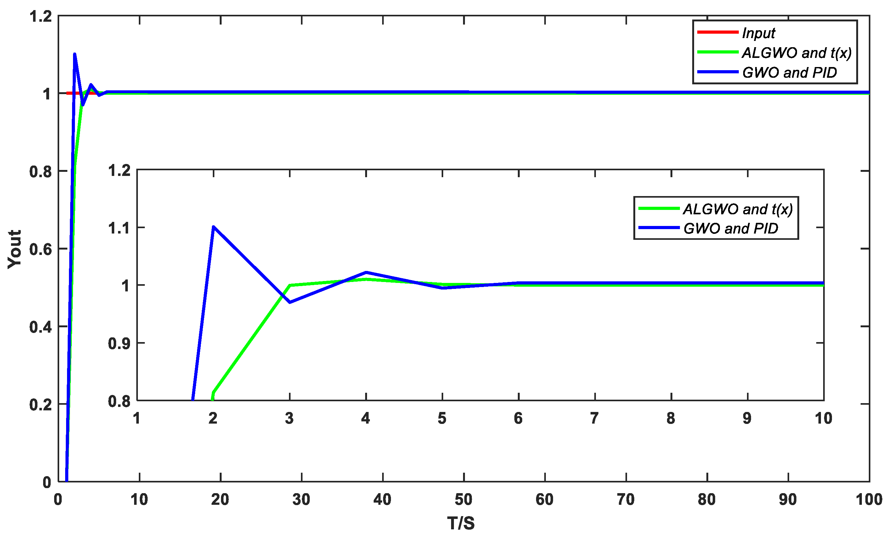
Figure 11.
Step response.
Figure 11.
Step response.
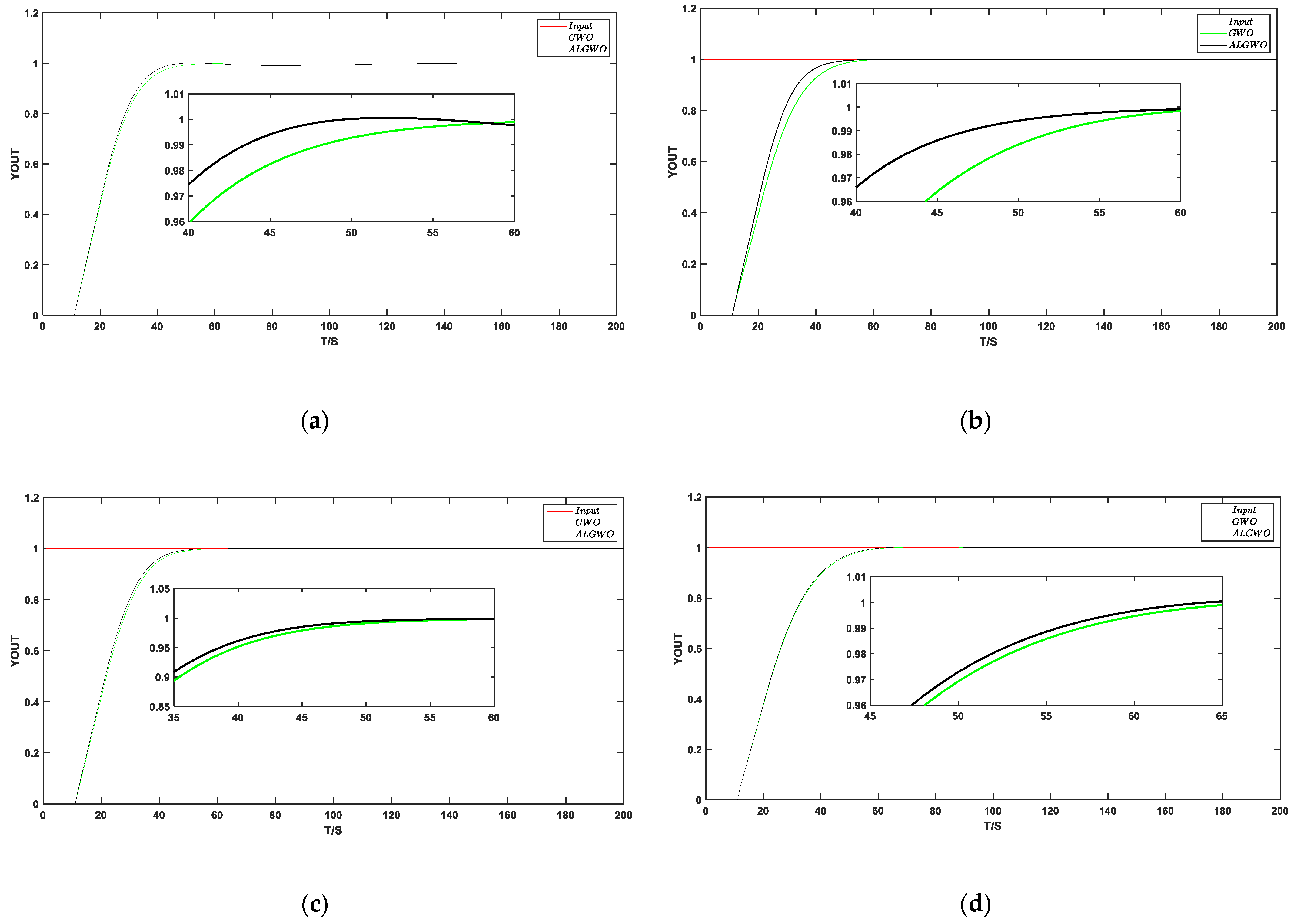
Figure 12.
The step response results on test system 5. (a) The simulation results of BPNN-PID using g(x) and (b) simulation results of BPNN-PID using t(x) and (c) simulation results of BPNN-PID using h(x) and (d) simulation results of traditional PID.
Figure 12.
The step response results on test system 5. (a) The simulation results of BPNN-PID using g(x) and (b) simulation results of BPNN-PID using t(x) and (c) simulation results of BPNN-PID using h(x) and (d) simulation results of traditional PID.
Figure 13.
The comparison results of algorithm optimization search on test system 5.
Figure 13.
The comparison results of algorithm optimization search on test system 5.
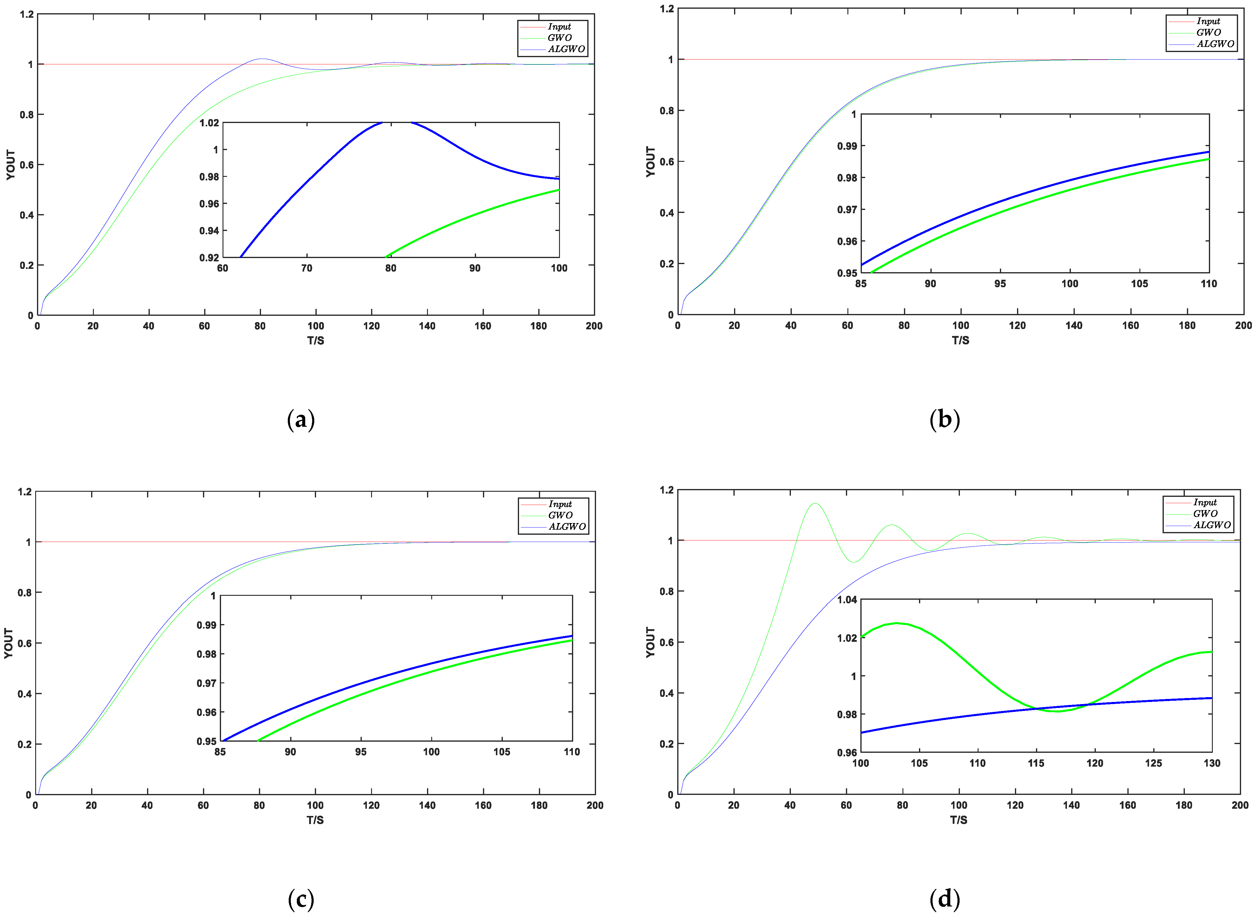
Figure 14.
The step response results on test system 6. (a) The simulation results of BPNN-PID using g(x) and (b) simulation results of BPNN-PID using t(x) and (c) simulation results of BPNN-PID using h(x) and (d) simulation results of traditional PID.
Figure 14.
The step response results on test system 6. (a) The simulation results of BPNN-PID using g(x) and (b) simulation results of BPNN-PID using t(x) and (c) simulation results of BPNN-PID using h(x) and (d) simulation results of traditional PID.
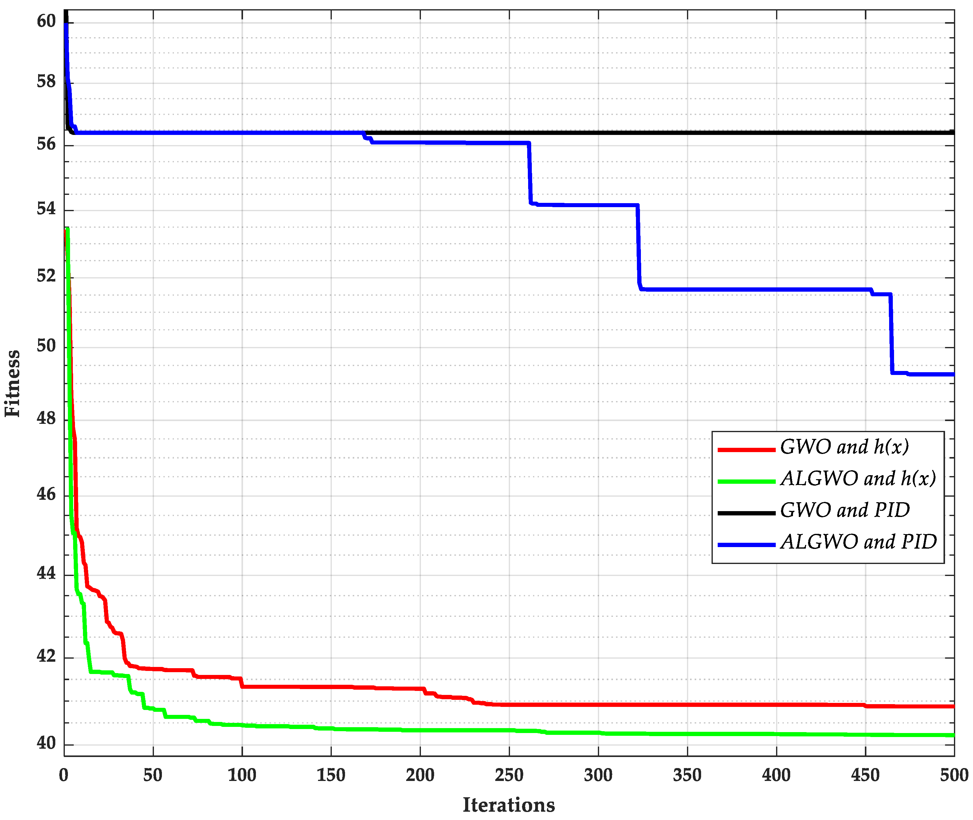
Figure 15.
The comparison results of algorithm optimization search on test system 6.
Figure 15.
The comparison results of algorithm optimization search on test system 6.
Table 1.
Parameter setups of different algorithms.
Table 1.
Parameter setups of different algorithms.
| Algorithm | Values of the Parameters |
| GWO | a = 2 (linear reduction during iteration) |
| SOGWO [38] | a = 2 (linear reduction during iteration) |
| PSO | |
| DE | F = 0.5, CR = 0.5 |
Table 2.
Details of the unimodal test function.
Table 2.
Details of the unimodal test function.
| Function Name | Expression | Search Space | Dim |
|---|
| F1 | | [−100,100] | 30 |
| F2 | | [−10,10] | 30 |
| F3 | | [−100,100] | 30 |
| F4 | | [−100,100] | 30 |
| F5 | | [−30,30] | 30 |
| F6 | | [−100,100] | 30 |
Table 3.
Comparison results of three algorithms on six groups of benchmark functions.
Table 3.
Comparison results of three algorithms on six groups of benchmark functions.
| Base Function | GWO | ALGWO | PSO |
|---|
| F1 | STD | 6.69 × 10−70 | 0 | 1.40 × 10⁻¹¹ |
| AVE | 2.49 × 10−70 | 0 | 5.48 × 10⁻¹² |
| F2 | STD | 3.49 × 10−41 | 0 | 1.01 × 10⁻⁵ |
| AVE | 3.89 × 10−41 | 3.01 × 10−238 | 7.24 × 10⁻⁶ |
| F3 | STD | 1.57 × 10⁻²⁰ | 0 | 3.47 × 100 |
| AVE | 8.72 × 10⁻²¹ | 0 | 7.16 × 100 |
| F4 | STD | 2.04 × 10⁻¹⁷ | 0 | 1.20 × 10⁻¹ |
| AVE | 1.77 × 10⁻¹⁷ | 2.70 × 10−206 | 3.90 × 10⁻¹ |
| F5 | STD | 8.78 × 10⁻¹ | 4.90 × 10⁻¹ | 3.46 × 101 |
| AVE | 2.66 × 101 | 2.62 × 101 | 5.04 × 101 |
| F6 | STD | 2.71 × 10⁻¹ | 1.09 × 100 | 1.59 × 10⁻¹¹ |
| AVE | 3.00 × 10⁻¹ | 3.58 × 10⁻¹ | 8.16 × 10⁻¹² |
Table 4.
Details of the multimodal test function.
Table 4.
Details of the multimodal test function.
| Function Name | Expression | Search Space | Dim |
|---|
| F8 | | [−500,500] | 30 |
| F9 | | [−5.12,5.12] | 30 |
| F10 | | [−32,32] | 30 |
| F11 | | [−600,600] | 30 |
Table 5.
Comparison results of five algorithms on four groups of benchmark functions.
Table 5.
Comparison results of five algorithms on four groups of benchmark functions.
| Base Function | GWO | ALGWO | SOGWO | PSO | DE |
|---|
| F8 | STD | 8.45 × 10² | 1.26 × 10³ | 7.11 × 10² | 8.35 × 10² | 6.86 × 10² |
| AVE | −5.98 × 10³ | −5.98 × 10³ | −6.44 × 10³ | −6.80 × 10³ | −5.97 × 10³ |
| F9 | STD | 0 | 0 | 0 | 8.22 × 100 | 1.57 × 101 |
| AVE | 0 | 0 | 0 | 3.47 × 101 | 2.57 × 10² |
| F10 | STD | 1.49 × 10⁻¹⁵ | 0 | 2.39 × 10⁻¹⁵ | 3.59 × 10⁻⁶ | 7.20 × 10⁻¹ |
| AVE | 1.43 × 10⁻¹⁴ | 4.44 × 10⁻¹⁵ | 1.40 × 10⁻¹⁴ | 2.56 × 10⁻⁶ | 1.72 × 10⁻¹ |
| F11 | STD | 0 | 0 | 0 | 7.30 × 10⁻³ | 2.67 × 100 |
| AVE | 0 | 0 | 0 | 7.10 × 10⁻³ | 3.63 × 10⁻¹ |
Table 6.
The comparison of final fitness of algorithms on test system 3.
Table 6.
The comparison of final fitness of algorithms on test system 3.
| Algorithm | | | | PID |
|---|
| GWO | AVE | 277.2945 | 295.4016 | 280.0701 | 301.2233 |
| STD | 13.5263 | 13.4028 | 13.5383 | 0.2515 |
| ALGWO | AVE | 275.7396 | 280.0453 | 278.7984 | 301.0937 |
| STD | 2.4216 | 12.3446 | 11.8726 | 0.2811 |
Table 7.
Performance characteristics on test system 4.
Table 7.
Performance characteristics on test system 4.
| Algorithm | Overshoot (%) | Rising Time (s) | Settling Time (s) | Fitness |
|---|
| GWO and | 0.62 | 3 | 3 | 1.0651 |
| GWO and | 0 | 2 | 4 | 1.0234 |
| GWO and | 0 | 2 | 2 | 1.0978 |
| GWO and PID | 10 | 2 | 3 | 11.9876 |
| ALGWO and | 0.02 | 2 | 3 | 1.0360 |
| ALGWO and | 0 | 2 | 4 | 1.0238 |
| ALGWO and | 0 | 2 | 2 | 1.0804 |
| ALGWO and PID | 6 | 2 | 4 | 11.8913 |
Table 8.
The comparison of final fitness of algorithms on test system 5.
Table 8.
The comparison of final fitness of algorithms on test system 5.
| Algorithm | | | | PID |
|---|
| GWO | AVE | 24.9222 | 25.0190 | 24.8169 | 27.0366 |
| STD | 0.6144 | 0.7097 | 0.6658 | 0.0773 |
| ALGWO | AVE | 24.1989 | 23.8964 | 24.8090 | 27.0068 |
| STD | 0.1029 | 0.1883 | 0.6113 | 0.0245 |
Table 9.
Performance characteristics on test system 5.
Table 9.
Performance characteristics on test system 5.
| Algorithm | Overshoot (%) | Rising Time (s) | Settling Time (s) | Fitness |
|---|
| GWO and | 0.06 | 34 | 41 | 24.2989 |
| GWO and | 0 | 38 | 49 | 25.0178 |
| GWO and | 0 | 35 | 44 | 24.7274 |
| GWO and PID | 0.18 | 41 | 52 | 26.9809 |
| ALGWO and | 0 | 35 | 45 | 24.2034 |
| ALGWO and | 0 | 34 | 44 | 23.9817 |
| ALGWO and | 0 | 30 | 36 | 24.2842 |
| ALGWO and PID | 0.11 | 41 | 53 | 26.9800 |
Table 10.
The comparison of final fitness of algorithms on test system 6.
Table 10.
The comparison of final fitness of algorithms on test system 6.
| Algorithm | | | | PID |
|---|
| GWO | AVE | 40.8749 | 46.6955 | 41.2529 | 56.4116 |
| STD | 0.61855 | 8.8126 | 1.2789 | 0 |
| ALGWO | AVE | 40.2174 | 41.1174 | 40.5169 | 49.2536 |
| STD | 0.5555 | 0.6698 | 0.6763 | 6.6099 |


