Article

Turbidity and COD Removal from Municipal Wastewater Using a TiO2 Photocatalyst—A Comparative Study of UV and Visible Light

Green Engineering Research Group, Department of Chemical Engineering, Faculty of Engineering and the Built Environment, Durban University of Technology, Durban 4001, South Africa
*
Author to whom correspondence should be addressed.
Appl. Sci. 2023, 13(8), 4766; https://doi.org/10.3390/app13084766
Submission received: 25 February 2023 / Revised: 24 March 2023 / Accepted: 4 April 2023 / Published: 10 April 2023

Abstract

:
Water resources are depleting, and the availability and supply of clean, potable water are a global concern. Advanced oxidation processes (AOPs) possess immense prospects in water and wastewater treatment settings. This study investigated and optimized the photocatalytic treatment of wastewater using titanium dioxide (TiO2) as the photocatalyst. The one-factor-at-a-time (OFAT) technique was employed to evaluate the effects of reaction time (20–100 min), mixing speed (20–100 rpm), and catalyst load (0.3–1.5 g/L) on pH, colour, turbidity, and chemical oxygen demand (COD) removal from actual municipal wastewater. Reaction time and catalyst load were then identified as the two key factors selected to be modeled and were optimized for turbidity and COD removal using the Central Composite Design (CCD) of response surface methodology (RSM). These statistical models were developed and used to optimize the operating conditions. The results obtained showed a desirability efficiency of 74.7% at a 95% confidence level. The RSM model predicted results at the optimum conditions and showed reasonable agreement with the experimental results obtained. The optimal responses achieved were 32.64% COD removal and 95.17% turbidity removal. A comparative study between UV light and visible light was also conducted at optimum conditions, whereby the UV light was demonstrated to be highly effective for turbidity and COD removal. The optimal responses achieved were 25.58% COD removal and 66.88% turbidity removal for visible light.

1. Introduction

The issue of water scarcity and how it can be solved continues to be a challenge to the world [1]. Herein, the continuous acceleration of water pollution due to population growth, urbanization, and industrialization, and the corresponding demand for non-renewable sources, has greatly increased [2]. Currently, South Africa’s municipalities are failing to provide clean water due to inadequate wastewater treatment facilities and limited or exhausted water resources. Piped water in two-thirds of South Africa’s municipalities do not meet minimum potable water standards [3,4,5]. The wastewater contains several contaminants, such as organic pollutants (dyes, phenolic compounds, surfactants, etc.), pathogenic microorganisms, and a range of different colloidal particles, which have harmful impacts on humans, animals, and the environment [6,7,8]. Their removal is therefore paramount. Several conventional wastewater treatment methods have been employed for decades. However, over the years, new and more challenging contaminants have emerged, and these contaminants have proven to be difficult to remove by traditional methods. Biological treatment methods commonly used are activated sludge and biofilm processes. However, high investment and operating costs, susceptibility to sludge swelling, and long pre-preparation cycles are the issues that exist in biological treatment processes [9]. Therefore, alternative and more advanced techniques are required [6,10]. Advanced oxidation processes (AOPs), an emerging wastewater treatment technology, displays great potential for the degradation of a variety of organic contaminants [2]. This process involves the generation of a highly reactive hydroxyl radical, which destroys the contaminants. Photocatalytic oxidation is a type of AOP whereby the photo-activated reactions are distinguished by the free radical mechanism initiated by the interaction of photons of an appropriate energy level with the catalyst [11].
Several researchers have investigated the use of photocatalysis for targeting individual pollutants. Most antibiotics are metabolized partially in the body, but 30% to 90% of them are discharged into the municipal sewage system without being metabolized [12,13]. Okhovat et al. [14] reported on the application of a photocatalytic process using nanoparticles for TiO2 on the removal of COD and metronidazole. The results on real wastewater (containing metronidazole at 80 mg/L and COD equal to 900 mg/L) showed that metronidazole and COD removal efficiencies at optimal conditions were 58.32% and 34.32%, respectively. Tayade et al. [15] found that an increase in catalyst load increased the decolourization and degradation percentages in their work to degrade methylene blue dye. However, the catalyst load may not exceed a certain quantity; otherwise, the degradation and decolourization percentages start to decrease due to light scattering and screening effects. This causes the catalyst’s surface to become unavailable for photon absorption. Furthermore, refs. [16,17,18,19] reported that excessive catalyst loading results in turbidity and a blocking effect that reduces light transmission through the whole solution and causes light scattering and a screening effect that decreases the degradation and decolourization percentages. The effect of light intensity is vital in the photocatalytic process, as the presence of sufficient light energy and wavelength allows for photocatalyst activation and enhances the generation of the hydroxyl and oxide radicals. In addition, refs. [16,17,20] stated that to achieve a high photocatalytic rate, specifically in water treatment, a reasonably high light intensity is required to sufficiently provide each TiO2 active site with enough photon energy. In addition to light intensity, light wavelength also affects the efficiency of photocatalytic degradation, especially when using common photocatalysts such as ZnO (zinc oxide), SnO2 (tin oxide), and TiO2, as they are only active when exposed to UV light, which accounts for only 5% of the solar spectrum or 388 nm [21]. As a result of their large bandgap (Eg > 3.0 eV), most photocatalysts are unable to take advantage of visible and infrared light, which accounts for 43% and 52% of solar energy, respectively. Additionally, refs. [22,23,24] stated that using commercial Degussa P-25, which has a crystalline ratio of anatase to rutile of 70/80:20/30 and a light wavelength of less than 380 nm, is adequate for photon activation. UV light provides a wavelength that ranges from 315 nm to 400 nm and therefore provides sufficient light photons for the photonic activation of the catalyst. Additionally, refs. [25,26,27,28,29] studied the effect of reaction time on the degradation efficiency of organic pollutants and found that an increase in reaction time increased the degradation efficiency, as the highest degradation efficiency was correlated to the longest reaction time. This was attributed to an increased interaction time between the pollutant and the surface of the photocatalyst. Farouq et al. [30] studied the effect of the mixing speed on the photocatalytic degradation of aqueous ammonia and found that an increase in mixing speed led to a higher percentage of ammonia removal. In addition, Yin et al. [31] also studied the effect of mixing speed with respect to decolourization and determined that when the mixing speed was increased, the bulk solution improved its transfer to the catalyst’s surface, therefore increasing decolourization.
The optimization of process parameters in the photocatalytic degradation process is complex and may require many experimental results. However, the Response Surface Methodology (RSM) employed in this study has the ability to produce a large amount of information from a limited number of experiments [32]. The numerical optimization technique will be utilized to ascertain the optimum conditions and interactions between the operating parameters.
The application of photocatalysis concerning the treatment of actual industrial wastewater is very limited [33]. In addition, the study explored the different light sources (UV and UV-visible) for the photocatalytic degradation of wastewater. In this study, the efficiency of TiO2 was studied and analyzed based on the removal of turbidity and chemical oxygen demand (COD) from actual municipal wastewater in a photo-catalytic system. Three operating parameters were varied: reaction time (20–100 min), mixing speed (20–100 rpm), and catalyst load (0.3–1.5 g/L), and their effect on pH, colour, turbidity, and COD removal from the wastewater was analyzed. RSM was used to optimize and study the interactions between the operating parameters using simulated wastewater by generating the values of the reaction time and catalyst load that produced the best (COD) removal and turbidity removal. These optimized parameters were then applied to UV/UV-Vis light sources, and a comparative study between the two light sources was performed to determine which light source achieved better results for COD and turbidity removal. The advantage of visible-light photocatalysis lies in its use of clean, renewable, and cheap visible light as a driving force. The sampled wastewater effluent used for the experiment was obtained from a local South African Municipal wastewater treatment plant.

2. Materials and Methods

2.1. Chemicals Used

CaCl2H2O, Peptone, Glucose, NaHCO3, Urea, Meat extract, MgSO4, K2HPO4, CuCl2.7H2O, NaCl and Titanium (IV) oxide were the chemicals used in the study. The characteristics of the commercial titanium dioxide used are as follows: the ratio of anatase to rutile is 75/25, particle size is 1–150 nm, density is 4.6 g/mol, and purity is 99%. All chemicals were supplied by Sigma Aldrich, Durban, South Africa.

2.2. Effluent Sample and Analytical Methods

2.2.1. Effluent Sample

Municipal wastewater from a local eThekwini municipality wastewater treatment plant based in Kwa-Zulu Natal, South Africa, was used. This wastewater was characterized and had the following characteristics: pH (6.85), colour (878 Pt.Co), turbidity (365 NTU), and COD (432 mg/L). The COD value was on the low side when the sample was taken. This municipality’s water was used for one factor at a time analysis. However, due to the limited availability of wastewater in the laboratory and the lack of consistency from the municipality’s treatment plant, synthetic wastewater was also simulated using analytical-grade chemicals that were mixed into a solution of 20 L of distilled water and 5 L of municipal wastewater. The composition of the chemicals used was adapted from Sibiya et al. [34] and is presented in Table 1. The synthetic wastewater was characterized for turbidity (317 NTU) and COD (870 mg/L). The COD value for synthetic water is higher than for the sample taken, which represents typical values for the treatment plant. This wastewater was used for RSM studies.

2.2.2. Analytical Methods

The pH and the turbidity were analyzed using the pH meter HI98130 and the turbidity meter HI98703-02, respectively (HANNA instruments). The COD and colour were analyzed by Spectrophotometer DR 3900 (HACH), using the stored programs 435- COD HR and 125- colour 465 nm. The COD and colour removal percentages were determined by using Equations (1) and (2), with the same equation set up applicable to turbidity percentage removal:
COD   removal   % = C i C f   C i   ×   100
where C i and C f are the initial and the final COD concentrations (mg/L) before and after treatment, respectively [35].
Colour   removal   % = C l i C l f C l i   ×   100
where C l i and C l f are the initial and the final Colour (Pt.Co) before and after treatment, respectively [36].

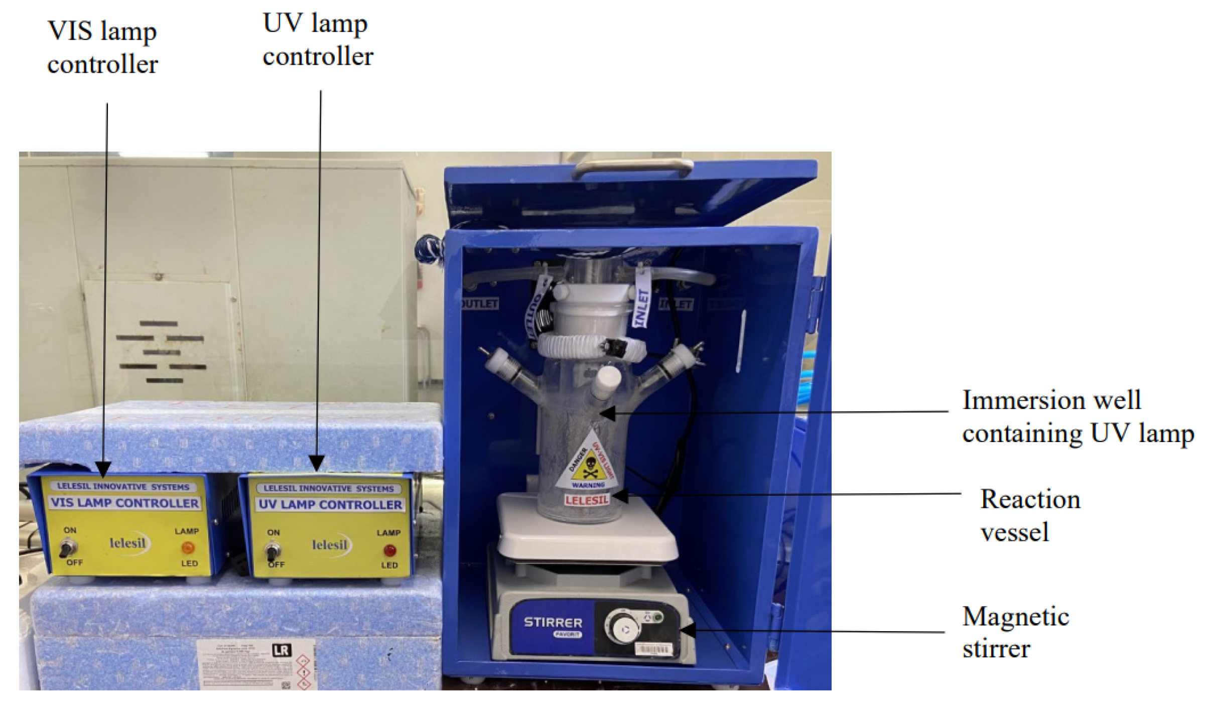
2.3. Experimental Setup

Figure 1 shows the set-up of a laboratory-scale photochemical reactor (Lelesil Innovative Systems). The photochemical reactor consists of a reaction vessel that has a 1.5 L capacity and an immersion well made of quartz, which houses the UV lamp. A cold-water circulating tank is used to cool down the immersion well that contains the lamp. A 250 W, 365 nm mercury UV and UV-Vis lamp was used.
As per the experimental design, experiments were performed based on one factor at a time. The first experiment varied reaction time from 20–100 min in increments of 20 min, whilst reaction speed and catalytic load remained constant at 60 rpm and 0.9 g/L, respectively. The second experiment varied mixing speed from 20–100 rpm in increments of 20 rpm, whilst reaction time and catalytic load remained constant at 30 min and 0.9 g/L, respectively. The third experiment varied catalyst load from 0.3–1.5 g/L in increments of 0.3 g/L, whilst reaction time and mixing remained constant at 30 min and 60 rpm, respectively. For each of the experiments, the reaction mixture was prepared by adding known amounts of TiO2 to municipal wastewater that was filled to just below the sample port of the reaction vessel, and samples were collected after a 10-min settling time was implemented after each increment. A similar set of experiments was performed; however, this time the input parameters generated by response surface methodology on design experts were used.

2.4. Response Surface Methodology (RSM)

Response surface methodology (RSM) was used in this study. RSM is a useful optimization tool for developing and studying the impact of independent and interactive factors in a process. These include process optimization, enhancement, and the development of products [25]. Essentially, RSM establishes the relationship between a variable and its effect (response), with the advantage of producing a mathematical model. The design of experiments was performed based on the central composite design (CCD) adopted from RSM using Design Expert (version 13.0.7) developed by Stat-Ease, Minneapolis, MN, USA. There were 2 numeric factors that generated 5 center points and 13 experimental runs (which were generated randomly). The two factors, reaction time and catalyst load, were assessed for two responses, turbidity removal and COD removal, and to the best of our knowledge, this is the first analysis that has been reported for municipality wastewater using these responses.

3. Results and Discussion

3.1. Characterization of Municipal Wastewater

The municipal wastewater properties are as follows: pH (6.85), colour (878 Pt.Co), turbidity (365 NTU), and COD (432 mg/L), as stated earlier, and these values were used as the basis for the analysis of the experimental results obtained.

3.2. Effect of Reaction Time on Photocatalysis Treatment

For this experiment, the effect of reaction time on the output parameters was studied. The reaction time was varied from 20 min to 100 min, while the mixing speed and catalyst load were kept constant at 60 rpm and 0.9 g/L, respectively. The reaction time had minimal effect on the pH (Figure 2a), as the pH values remained almost constant, ranging from 6.79 to 7.11, further validating the minimal effect reaction time had on pH, as the pH also remained close to the characterized wastewater pH of 6.85. Constant pH suggests that the products of photocatalysis had no significant influence on pH.
The removal efficiencies of the parameters colour (Figure 2b), turbidity (Figure 2c), and COD (Figure 2d) were highest in the first 20 min and then decreased thereafter. The initial increase is because, with an increase in contact time, the availability of hydroxyl radicals for the oxidation of pollutants present in wastewater increases [35]. Kumar and Pandey [29] studied the effect of reaction time on the photodegradation of methyl green and also found that an increase in reaction time increased the degradation efficiency, which they attributed to increased interaction time between the pollutant and the surface of the photocatalyst. The decrease thereafter might be because the TiO2 photocatalyst aggregated with the pollutants, and with time, the interactive surface of the photocatalyst became saturated and dissociated, contributing to secondary complex pollutants [15,16].

3.3. Effect of Mixing Speed on Photocatalysis Treatment

For this experiment, the effect of mixing speed on the output parameters was studied. The mixing speed was varied from 20 rpm to 100 rpm while the reaction time and catalyst load were kept constant at 30 min and 0.9 g/L, respectively. The mixing speed had minimal effect on the pH (Figure 3a), as the values remained constant, ranging from 6.77 to 7.39. Farouq et al. [30] studied the effect of the mixing speed on the photocatalytic degradation of aqueous ammonia and found that an increasing mixing speed leads to a higher percentage of ammonia removal. In contrast to this, as the mixing speed increased, the removal efficiencies for colour (Figure 3b), turbidity (Figure 3c), and COD (Figure 3d) decreased. So it is believed that as stirring speed is increased, TiO2 particles disintegrate, contributing to an increase in the three parameters [37].

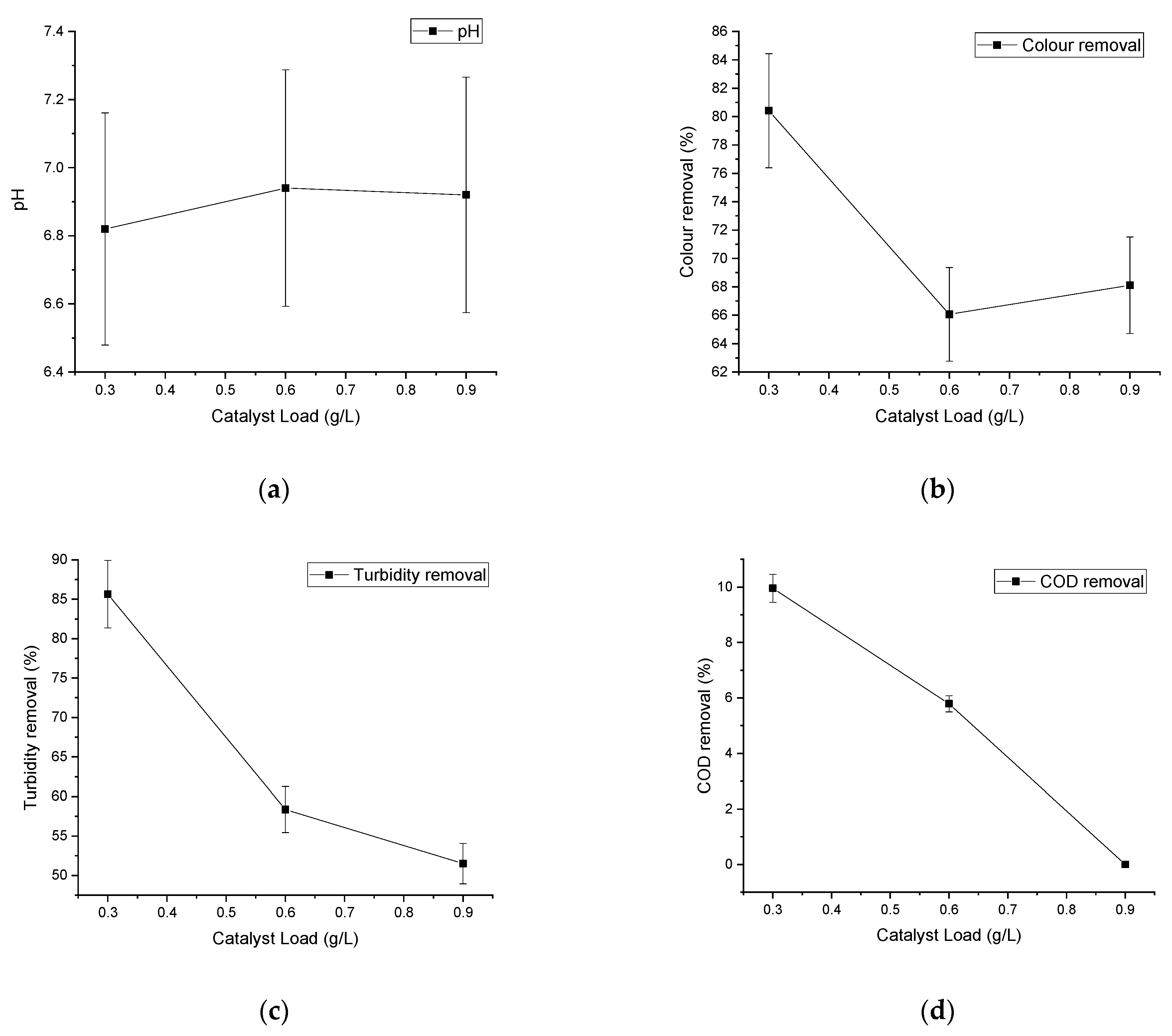
3.4. Effect of Catalyst Load on Photocatalysis Treatment

For this experiment, the effect of catalyst load on the output parameters was studied. The catalyst load was varied from 0.3 g/L to 1.5 g/L, while the reaction time and mixing speed were kept constant at 30 min and 60 rpm, respectively. The catalyst load had a minimal effect on the pH (Figure 4a), as no significant change in pH was observed; it ranged from 6.82 to 7.24. The catalyst load removal efficiency results for colour (Figure 4b), turbidity (Figure 4c), and COD (Figure 4d) decreased with an increase in catalyst load. These results concur with the findings of previous researchers [15,19], who reported that removal efficiencies decreased above the optimum catalyst load. Mecha et al. [38] investigated the effect of catalyst concentrations (0.1, 0.5, and 1.0 g/L) and reported that the percentage removal of phenol increased with catalyst loading until 0.5 g/L and thereafter decreased at higher catalyst loading. Furthermore, refs. [16,17,19] found that excessive catalyst loading results in turbidity and a blocking effect that reduces light transmission through the whole solution and causes light scattering and a screening effect that decreases the degradation and decolourization percentages.
It was observed that reaction time and catalyst load, turbidity, and COD removal were the most significant input and output variables, respectively, and therefore these were the parameters used for the optimization. Furthermore, the optimal ranges for catalyst load and reaction time were determined to be 0.3–0.6 g/L and 20–40 min, respectively. These conditions were applied to the optimization.

3.5. Previous Similar Work

The TiO2 treatment achieved high removal efficiencies for turbidity and colour removal. A comparison with other actual wastewater studies from different wastewater sources shows that the removal efficiency for COD was very low in this work (Table 2). The removal of COD is an important indicator for evaluating the mineralization degree of the system [39]. The low activity in COD removal in this work will suggest that TiO2 usage for treating eThekwini municipality wastewater could face challenges if used as a standalone technology. The difference in removal efficiencies between this work and the literature may be due to the difference in the wastewater composition. This will lead to different potential scavengers in the systems, and therefore, researchers are encouraged to do a more detailed analysis of the wastewater to include potential scavengers. Another potential cause of low activity is the number of ions dissolved in the wastewater (ionic strength). In the presence of strong electrolytes, the solubility of oxygen is lower than in pure water [40], hence lower activity.

3.6. Response Surface Modelling and Optimization
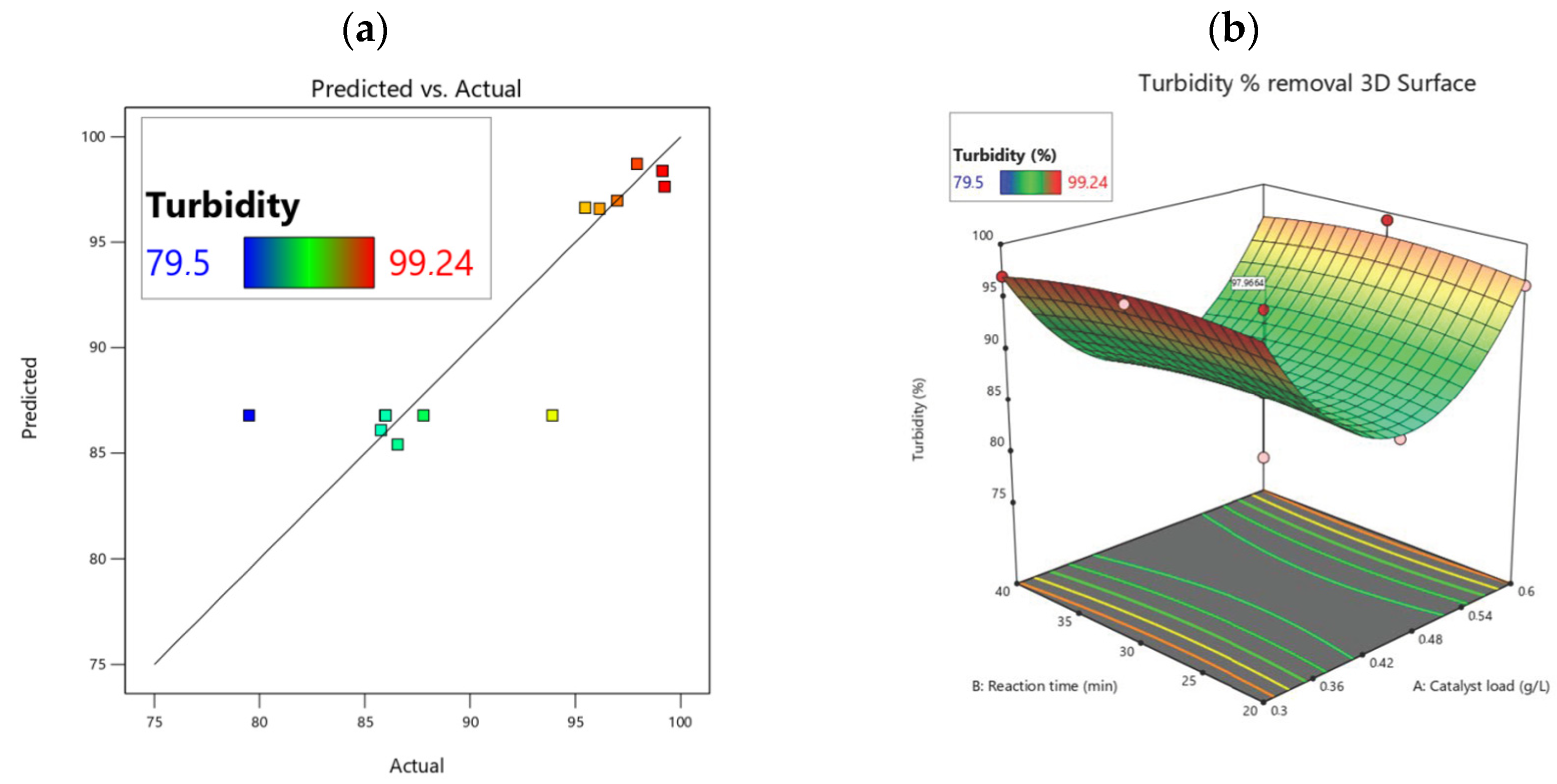
3.6.1. Turbidity

Synthetic wastewater was characterized and used for the RSM experimental runs. Turbidity and COD were 317 NTU and 870 mg/L. Table 3 shows the operating parameters (factor 1 and factor 2) generated by RSM. Once these runs were conducted, the results for the output parameters were entered. Next, the two responses were then analyzed by the Design Expert.
The fit summary for response 1, shown in Table 4, was generated, and the quadratic model was suggested based on the p-value; see Equation (3).
The results for the analysis of variance (ANOVA) for the quadratic model can be seen in Table 5, and the model F-value of 4.91 indicates the model is significant. It also suggests that an F-value this large only has a 3.01% chance of occurring due to noise. The p-value generated is 0.0301 and indicates that the model term is significant as it is less than 0.0500. Specific to this case, A2 is a significant model term. Any p-value that is greater than 0.1000 suggests the model terms are not significant; however, hierarchy terms are not included in the terms counted. Therefore, this model is significant and acceptable as only model terms AB and B2 are above 0.100. Lastly, the value of 0.9639 for the lack of fit indicates that it is not significant relative to pure error, and a non-significant lack of fit value indicates that the model will fit. The predicted R2 value of 0.5647 is in reasonable agreement with the adjusted R2 value of 0.6196, as the difference between the two values is less than 0.2. The adequate precision (Adeq. Pr) of 4.8711 shows an adequate signal as the value is greater than 4, which is desirable.
The predicted values were plotted against the experimental values using an experimental predicted data interactive plot to approximate the extent of the correlation. Figure 5a depicts a reasonably strong linear correlation between the experimental and predicted data with a high regression coefficient (Table 5), with only a couple of data points as outliers. The standard error (SE) for the line of best fit showed an insignificant deviation, as the p-value was less than 0.05 at a 95% confidence level. The modified RSM and Central Composite Design (CCD) (RSM-CCD) were used to demonstrate the interactive impact of the input parameters (factors) on the output parameters (response). Figure 5b displays the presence of interactions between the factors, catalyst load, and reaction time on the turbidity response. The graphical demonstration of the three-dimensional (3D) surface plot of the response model was selected based on the interaction of the significant factors that play a role in maximizing the desirability of the system. A curvature of considerable magnitude can be seen in Figure 5b. This curve also suggests that the correlation between the factors (AB) and the response (turbidity) were well-fitted on a quadratic function (Equation (3)). Graphically (Figure 5b), it was demonstrated that the response surface showed an arc with the optimal region for turbidity at the high-low levels of A (catalyst load), whilst the turbidity removal remained constant along the varying reaction times and therefore did not have as significant an effect as the catalyst load.
Turbidity = 86.79 − 0.5333A − 0.3417B + 0.3650AB + 11.38A2 − 1.03B2

3.6.2. COD

The fit summary for response 2, shown in Table 6, was generated, and the quadratic model was suggested in Equation (4).
The results for the analysis of variance (ANOVA) for the quadratic model can be seen in Table 7, and they suggest that the Model F-value of 6.85 indicates the model is significant. It also suggests that an F-value this large only has a 1.06% chance of occurring due to noise. The p-value generated is 0.0106 and indicates that the model term is significant as it is less than 0.0500. Any p-value that is greater than 0.1000 suggests the model terms are not significant; however, hierarchy terms are not included in the terms counted. Therefore, this model is significant and acceptable, as only model term B is above 0.100. Lastly, the value of 0.6632 for the lack of fit indicates that it is not significant relative to pure error, and a non-significant lack of fit value indicates that the model will fit. Table 7 indicates that the predicted R2 value of 0.4378 is in reasonable agreement with the adjusted R2 value of 0.5939, as the difference between the two values is less than 0.2. The Adeq. Pr of 6.0593 shows an adequate signal as the value is greater than 4, which is desirable.
The predicted values were plotted against the experimental values using an experimental predicted data interactive plot to approximate the extent of the correlation. Figure 6a shows that only a few data points were recurrently scattered around the line of best fit, which could explain the inconsistent COD % removal (organic degradation) based on the specified experimental conditions. The standard error for the line of best fit showed an insignificant deviation with a p-value less than 0.05 at a 95% confidence level. The COD model regression is low (Table 7) despite the model’s adjusted and predicted R2 values being in reasonable agreement with a difference of less than 0.2. A curvature of considerable magnitude can be seen in Figure 6b. This curve also suggests that the correlation between the factors (AB) and the response (COD) was well fitted to a quadratic function (4). Graphically (Figure 6b), it was demonstrated that the response surface showed an arc with the optimal region for turbidity at the higher levels of A (catalyst load), ranging from 0.48 g/L to 0.54 g/L, whilst the COD removal remained constant along the varying reaction time and therefore did not have as significant an effect as the catalyst load.
COD = 35.88 + 14.27𝐴 + 1.55𝐵 − 18.62𝐴2

3.6.3. Optimization Using RSM

To optimize the experimental design, constraints (Table 8) had to be implemented. Specific to this case, all input and output parameters (factors and responses) were maximized. This generated 8 solutions (Table 9), and one was selected as the optimal solution (Figure 7) as it presented the highest desirability of 74.7% removal efficiency. The optimal solution suggests a turbidity and COD removal of 96.6% and 33.1%, respectively, were attained at a catalyst load of 0.6 g/L and a reaction time of 40 min.

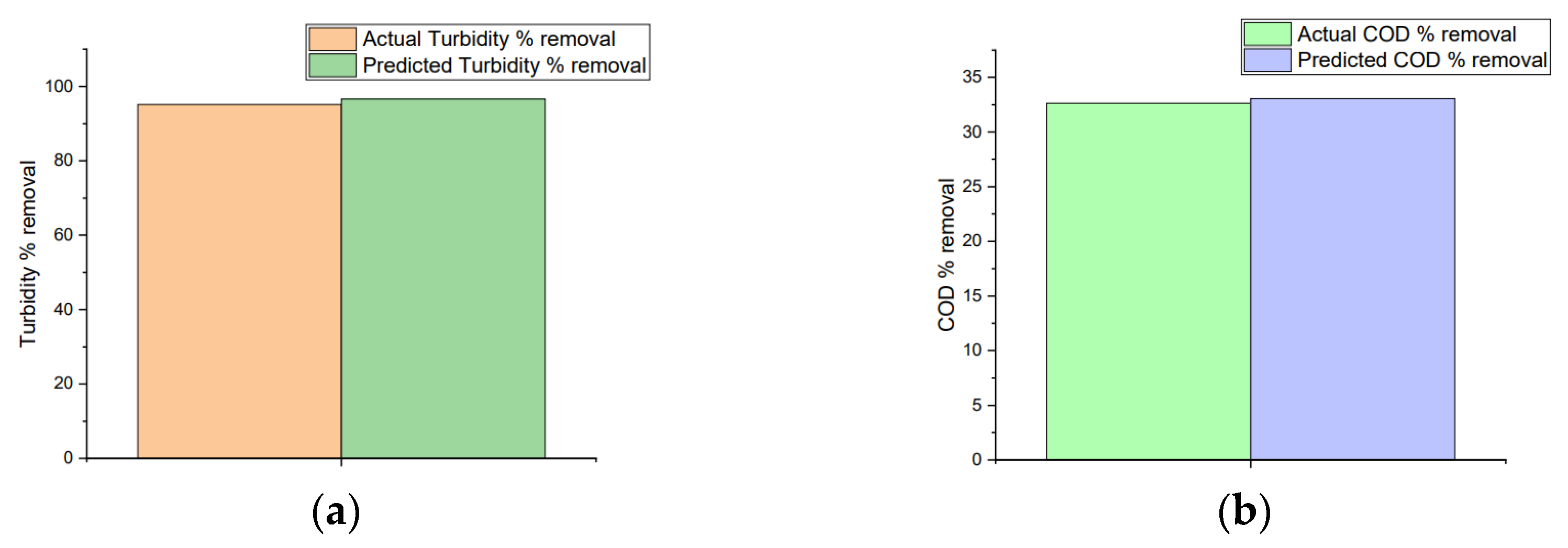
3.6.4. Validation of Optimized Conditions

The selected optimal conditions were validated and confirmed experimentally (Table 10) and were in good agreement with the predicted values, as the difference between the predicted and actual values was minimal (Figure 8a,b). This suggests the model’s predictability was consistent (p < 0.05) at 95% confidence levels.
It was also determined, according to the South African National Standards (SANS) 241 and the South African wastewater and industrial effluent law (2013), that the COD output parameter (498 mg/L) met the standards, whilst the turbidity output parameter (15.3 NTU) did not. This might be due to the syringe filter not being able to completely remove all TiO2 nanoparticles. We observed a low value for COD removal, and these results are consistent with what was observed by Okhovat et al. [14], who observed a 34.32% COD removal. The potential reasons for a low COD removal are discussed in Section 3.5, and this could be due to scavengers and the high ionic strength of the wastewater.

3.7. Comparative Study between UV and Vis Light

Finally, once the optimal operating parameters were verified, a comparative study was performed, whereby the same experiment was conducted using UV-Vis light. The turbidity and COD removal percentages obtained under UV-Vis irradiation are lower than those obtained under UV irradiation. The optimal responses achieved for this were 25.58% COD removal and 66.88% turbidity removal. This is possibly due to TiO2 not being photoexcited by visible light due to its large energy band gap [22], and this is in line with the literature [45]. Due to turbidity caused by TiO2 particles, additional post-treatment separation methods are required. Further studies making use of TiO2 as a catalyst for photocatalytic wastewater treatment should include additional post-treatment filtration steps to recover the TiO2 to ensure optimal removal of the nanoparticles and to enhance turbidity and COD removal.

4. Conclusions

The one-factor-at-a-time method revealed that the two operating parameters, reaction time and catalyst load, had a significant effect on two output parameters, turbidity and COD removal. Furthermore, the optimal ranges for catalyst load and reaction time were established to be 0.3–0.6 g/L and 20–40 min, respectively. These conditions were then applied to the optimization technique. The Central Composite Design (CCD) matrix of 13 experimental runs and 5 center points, with reaction time (20–40 min) and catalyst load (0.3–0.6 g/L) as the 2 input variables, were developed at their low, high, and middle points. RSM was used to model and optimize the input-output variable relationship. The analysis of variance (ANOVA) revealed that all models generated were significant as they possessed a p-value less than 0.05 at a 95% confidence level. Therefore, this signifies good predictability for the optimization of the process. A desirability of 74.7% was achieved at optimal conditions of 0.6 g/L for catalyst load and 40 min for reaction time. The predicted results from RSM were found to be in good agreement with the experimental results. The optimal responses achieved were 32.64% COD removal and 95.17% turbidity removal. The optimal conditions were also applied to the comparative experiment that utilized UV-Vis light instead of UV light. The optimal responses achieved for this were 25.58% COD removal and 66.88% turbidity removal. This is possibly due to TiO2 not being photoexcited by visible light due to its large energy band gap. Due to the turbidity of the TiO2, additional post-treatment separation methods are required. Further studies making use of TiO2 as a catalyst for photocatalytic wastewater treatment should include additional post-treatment filtration steps to recover the TiO2 to ensure optimal removal of the nanoparticles and to enhance turbidity and COD removal. The use of actual wastewater highlighted the need for better characterization of wastewater for better comparison and explanation of variation in removal efficiencies of different systems.

Author Contributions

Conceptualization, E.K.T., S.R., S.J., C.M. and T.G.; methodology, S.J., C.M. and T.G.; software, S.J., C.M. and T.G.; validation, S.J., C.M. and T.G.; formal analysis, C.M. and T.G.; investigation, C.M. and T.G.; resources, S.R. and E.K.T.; data curation, C.M. and T.G.; writing—original draft preparation, S.J., C.M. and T.G.; writing—review and editing, L.L.M., S.R. and E.K.T.; visualization, C.M.; supervision, S.R. and E.K.T.; project administration, S.R. and E.K.T. All authors have read and agreed to the published version of the manuscript.

Funding

This project was supported by the South African Water Research Commission (WRC Project: C2021/2022-00958).

Institutional Review Board Statement

Not applicable.

Data Availability Statement

Data is contained within the article.

Acknowledgments

The authors are thankful to the Green Engineering Research Group, Department of Chemical Engineering, Durban University of Technology, and eThekwini municipality for their support.

Conflicts of Interest

The authors declare no conflict of interest.

References

  1. du Plessis, A. South Africa’s Impending Water Crises: Transforming Water Crises into Opportunities and the Way Forward. In South Africa’s Water Predicament: Freshwater’s Unceasing Decline; Springer: Berlin/Heidelberg, Germany, 2023; pp. 143–170. [Google Scholar]
  2. Zhang, F.; Wang, X.; Liu, H.; Liu, C.; Wan, Y.; Long, Y.; Cai, Z. Recent Advances and Applications of Semiconductor Photocatalytic Technology. Appl. Sci. 2019, 9, 2489. [Google Scholar] [CrossRef] [Green Version]
  3. Kretzmann, S. Municipalities Are Failing to Provide Clean Water. Citizens Are Stepping in to Fix the Problem. Available online: https://www.groundup.org.za/article/water-in-two-thirds-municipalities-does-not-meet-minimum-standards/ (accessed on 6 March 2023).
  4. Toxopeüs, M. Understanding Water Issues and Challenges II: Municipalities and the Delivery of Water Services. Available online: https://hsf.org.za/publications/hsf-briefs/understanding-water-issues-and-challenges-ii-municipalities-and-the-delivery-of-water-services (accessed on 1 December 2022).
  5. Xaba, N. The Centrality of the Water-Energy-Food Nexus in Navigating South Africa’s Power Crisis. Available online: https://www.dailymaverick.co.za/opinionista/2023-02-27-the-water-energy-food-nexus-and-south-africas-energy-crisis/ (accessed on 10 March 2023).
  6. Antonopoulou, M.; Papadopoulos, V.; Konstantinou, I. Photocatalytic Oxidation of Treated Municipal Wastewaters for the Removal of Phenolic Compounds: Optimization and Modeling Using Response Surface Methodology (RSM) and Artificial Neural Networks (ANNS). J. Chem. Technol. Biotechnol. 2012, 87, 1385–1395. [Google Scholar] [CrossRef]
  7. Jabbar, Z.H.; Graimed, B.H. Recent Developments in Industrial Organic Degradation Via Semiconductor Heterojunctions and the Parameters Affecting the Photocatalytic Process: A Review Study. J. Water Process Eng. 2022, 47, 102671. [Google Scholar] [CrossRef]
  8. Archer, E.; Wolfaardt, G.M.; Van Wyk, J.H. Pharmaceutical and Personal Care Products (PPCPS) as Endocrine Disrupting Contaminants (EDCS) in South African Surface Waters. Water SA 2017, 43, 684–706. [Google Scholar] [CrossRef] [Green Version]
  9. Ma, D.; Yi, H.; Lai, C.; Liu, X.; Huo, X.; An, Z.; Li, L.; Fu, Y.; Li, B.; Zhang, M. Critical Review of Advanced Oxidation Processes in Organic Wastewater Treatment. Chemosphere 2021, 275, 130104. [Google Scholar] [CrossRef] [PubMed]
  10. Manna, M.; Sen, S. Advanced Oxidation Process: A Sustainable Technology for Treating Refractory Organic Compounds Present in Industrial Wastewater. Environ. Sci. Pollut. Res. 2022, 30, 25477–25505. [Google Scholar] [CrossRef]
  11. Thiruvenkatachari, R.; Vigneswaran, S.; Moon, I.S. A Review on UV/TiO 2 Photocatalytic Oxidation Process. Korean J. Chem. Eng. 2008, 25, 64–72. [Google Scholar] [CrossRef]
  12. Vieno, N.; Tuhkanen, T.; Kronberg, L. Elimination of Pharmaceuticals in Sewage Treatment Plants in Finland. Water Res. 2007, 41, 1001–1012. [Google Scholar] [CrossRef]
  13. Ben, W.; Qiang, Z.; Pan, X.; Chen, M. Removal of Veterinary Antibiotics from Sequencing Batch Reactor (SBR) Pretreated Swine Wastewater by Fenton’s Reagent. Water Res. 2009, 43, 4392–4402. [Google Scholar] [CrossRef]
  14. Okhovat, N.; Hashemi, M.; Golpayegani, A. Photocatalytic Decomposition of Metronidazolein Aqueous Solutions Using Titanium Dioxide Nanoparticles. J. Mater. Environ. Sci. 2015, 6, 792–799. [Google Scholar]
  15. Tayade, R.J.; Natarajan, T.S.; Bajaj, H.C. Photocatalytic Degradation of Methylene Blue Dye Using Ultraviolet Light Emitting Diodes. Ind. Eng. Chem. Res. 2009, 48, 10262–10267. [Google Scholar] [CrossRef]
  16. Al-Nuaim, M.A.; Alwasiti, A.A.; Shnain, Z.Y. The Photocatalytic Process in the Treatment of Polluted Water. Chem. Pap. 2022, 77, 677–701. [Google Scholar] [CrossRef] [PubMed]
  17. Jing, B.; Chow, C.; Saint, C. Recent Developments in Photocatalytic Water Treatment Technology. Water Res. 2010, 44, 2997–3027. [Google Scholar]
  18. Friedmann, D. A General Overview of Heterogeneous Photocatalysis as a Remediation Technology for Wastewaters Containing Pharmaceutical Compounds. Water 2022, 14, 3588. [Google Scholar] [CrossRef]
  19. Jallouli, N.; Pastrana-Martínez, L.M.; Ribeiro, A.R.; Moreira, N.F.; Faria, J.L.; Hentati, O.; Silva, A.M.; Ksibi, M. Heterogeneous Photocatalytic Degradation of Ibuprofen in Ultrapure Water, Municipal and Pharmaceutical Industry Wastewaters Using a TiO2/UV-LED System. Chem. Eng. J. 2018, 334, 976–984. [Google Scholar] [CrossRef]
  20. Chiou, C.-H.; Wu, C.-Y.; Juang, R.-S. Influence of Operating Parameters on Photocatalytic Degradation of Phenol in UV/TiO2 Process. Chem. Eng. J. 2008, 139, 322–329. [Google Scholar] [CrossRef]
  21. Yakout, S. New Efficient Sunlight Photocatalysts Based on Gd, Nb, V and Mn Doped Alpha-Bi2O3 Phase. J. Environ. Chem. Eng. 2020, 8, 103644. [Google Scholar] [CrossRef]
  22. Zare, E.N.; Iftekhar, S.; Park, Y.; Joseph, J.; Srivastava, V.; Khan, M.A.; Makvandi, P.; Sillanpaa, M.; Varma, R.S. An Overview on Non-Spherical Semiconductors for Heterogeneous Photocatalytic Degradation of Organic Water Contaminants. Chemosphere 2021, 280, 130907. [Google Scholar] [CrossRef]
  23. Herrmann, J.-M. Heterogeneous Photocatalysis: Fundamentals and Applications to the Removal of Various Types of Aqueous Pollutants. Catal. Today 1999, 53, 115–129. [Google Scholar] [CrossRef]
  24. Bahnemann, D. Photocatalytic Water Treatment: Solar Energy Applications. Sol. Energy 2004, 77, 445–459. [Google Scholar] [CrossRef]
  25. Bhatkhande, D.S.; Kamble, S.P.; Sawant, S.B.; Pangarkar, V.G. Photocatalytic and Photochemical Degradation of Nitrobenzene Using Artificial Ultraviolet Light. Chem. Eng. J. 2004, 102, 283–290. [Google Scholar] [CrossRef]
  26. Chin, S.S.; Chiang, K.; Fane, A.G. The Stability of Polymeric Membranes in a TiO2 Photocatalysis Process. J. Membr. Sci. 2006, 275, 202–211. [Google Scholar] [CrossRef]
  27. Ochuma, I.J.; Fishwick, R.P.; Wood, J.; Winterbottom, J.M. Optimisation of Degradation Conditions of 1, 8-Diazabicyclo [5.4. 0] Undec-7-Ene in Water and Reaction Kinetics Analysis Using a Cocurrent Downflow Contactor Photocatalytic Reactor. Appl. Catal. B Environ. 2007, 73, 259–268. [Google Scholar] [CrossRef]
  28. Shivaraju, H. Removal of Organic Pollutants in the Municipal Sewage Water by TiO2 Based Heterogeneous Photocatalysis. Int. J. Environ. Sci. 2011, 1, 911–923. [Google Scholar]
  29. Kumar, A.; Pandey, G. The Photocatalytic Degradation of Methyl Green in Presence of Visible Light with Photoactive Ni0. 10: La0. 05: TiO2 Nanocomposites. IOSR J. Appl. Chem. 2017, 10, 31–44. [Google Scholar]
  30. Farouq, R.; Abd-Elfatah, M.; Ossman, M.E. Response Surface Methodology for Optimization of Photocatalytic Degradation of Aqueous Ammonia. J. Water Supply Res. Technol.–AQUA 2018, 67, 162–175. [Google Scholar] [CrossRef]
  31. Yin, X.; Xin, F.; Zhang, F.; Wang, S.; Zhang, G. Kinetic Study on Photocatalytic Degradation of 4BS Azo Dye Over TiO2 in Slurry. Environ. Eng. Sci. 2006, 23, 1000–1008. [Google Scholar] [CrossRef]
  32. Goren, A.Y.; Recepoğlu, Y.K.; Khataee, A. Language of Response Surface Methodology as an Experimental Strategy for Electrochemical Wastewater Treatment Process Optimization. In Artificial Intelligence and Data Science in Environmental Sensing; Elsevier: Amsterdam, The Netherlands, 2022; pp. 57–92. [Google Scholar]
  33. Das, A.; Adak, M.K.; Mahata, N.; Biswas, B. Wastewater Treatment with the Advent of TiO2 Endowed Photocatalysts and their Reaction Kinetics with Scavenger Effect. J. Mol. Liq. 2021, 338, 116479. [Google Scholar] [CrossRef]
  34. Sibiya, N.P.; Rathilal, S.; Kweinor Tetteh, E. Coagulation Treatment of Wastewater: Kinetics and Natural Coagulant Evaluation. Molecules 2021, 26, 698. [Google Scholar] [CrossRef]
  35. Syed, M.A.; Mauriya, A.K.; Shaik, F. Investigation of Epoxy Resin/Nano-TiO2 Composites in Photocatalytic Degradation of Organics Present in Oil-Produced Water. Int. J. Environ. Anal. Chem. 2022, 102, 4518–4534. [Google Scholar] [CrossRef]
  36. Shankar, D.; Sivakumar, D.; Thiruvengadam, M.; Manojkumar, M. Colour Removal in a Textile Industry Wastewater Using Coconut Coir Pith. Pollut. Res. 2014, 33, 499–503. [Google Scholar]
  37. Govindaraj, M.; Pattabhi, S. Electrochemical Treatment of Endocrine-Disrupting Chemical from Aqueous Solution. Desalination Water Treat. 2015, 53, 2664–2674. [Google Scholar] [CrossRef]
  38. Mecha, A.C.; Onyango, M.S.; Ochieng, A.; Jamil, T.S.; Fourie, C.J.; Momba, M.N. UV and Solar Light Photocatalytic Removal of Organic Contaminants in Municipal Wastewater. Sep. Sci. Technol. 2016, 51, 1765–1778. [Google Scholar] [CrossRef]
  39. Gao, B.; Liu, L.; Liu, J.; Yang, F. Photocatalytic Degradation of 2, 4, 6-Tribromophenol on Fe2O3 or FeOOH Doped ZnIn2S4 Heterostructure: Insight into Degradation Mechanism. Appl. Catal. B Environ. 2014, 147, 929–939. [Google Scholar] [CrossRef]
  40. Zheng, P.; Pan, Z.; Li, H.; Bai, B.; Guan, W. Effect of Different Type of Scavengers on the Photocatalytic Removal of Copper and Cyanide in the Presence of TiO2 @ Yeast Hybrids. J. Mater. Sci. Mater. Electron. 2015, 26, 6399–6410. [Google Scholar] [CrossRef]
  41. Chong, M.N.; Cho, Y.J.; Poh, P.E.; Jin, B. Evaluation of Titanium Dioxide Photocatalytic Technology for the Treatment of Reactive Black 5 Dye in Synthetic and Real Greywater Effluents. J. Clean. Prod. 2015, 89, 196–202. [Google Scholar] [CrossRef]
  42. Tetteh, E.K.; Obotey Ezugbe, E.; Rathilal, S.; Asante-Sackey, D. Removal of COD and SO42− from Oil Refinery Wastewater Using a Photo-Catalytic System—Comparing TiO2 and Zeolite Efficiencies. Water 2020, 12, 214. [Google Scholar] [CrossRef] [Green Version]
  43. Topare, N.S.; Joy, M.; Joshi, R.R.; Jadhav, P.B.; Kshirsagar, L.K. Treatment of Petroleum Industry Wastewater Using TiO2/UV Photocatalytic Process. J. Indian Chem. Soc. 2015, 92, 219–222. [Google Scholar]
  44. Ghaly, M.Y.; Jamil, T.S.; El-Seesy, I.E.; Souaya, E.R.; Nasr, R.A. Treatment of Highly Polluted Paper Mill Wastewater by Solar Photocatalytic Oxidation with Synthesized Nano TiO2. Chem. Eng. J. 2011, 168, 446–454. [Google Scholar] [CrossRef]
  45. Madkhali, N.; Prasad, C.; Malkappa, K.; Choi, H.Y.; Govinda, V.; Bahadur, I.; Abumousa, R. Recent Update on Photocatalytic Degradation of Pollutants in Waste Water Using TiO2-Based Heterostructured Materials. Results Eng. 2023, 17, 100920. [Google Scholar] [CrossRef]
Figure 1. Photocatalytic wastewater treatment experimental set-up.
Applsci 13 04766 g001
Figure 2. Trends of the effect of reaction time on photocatalysis treatment parameters: (a) The effect of reaction time on pH; (b) The effect of reaction time on colour removal; (c) The effect of reaction time on turbidity removal (d) The effect of reaction time on COD removal (mixing speed at 60 rpm and catalyst loading at 0.9 g/L).
Applsci 13 04766 g002
Figure 3. Trends of the effect of mixing speed on photocatalysis treatment parameters: (a) The effect of mixing speed on pH; (b) The effect of mixing speed on colour removal; (c) The effect of mixing speed on turbidity removal (d) The effect of mixing speed on COD removal (reaction time of 30 min and catalyst loading of 0.9 g/L).
Applsci 13 04766 g003
Figure 4. Trends of the effect of catalyst load on photocatalysis treatment parameters: (a) The effect of catalyst load on pH; (b) The effect of catalyst load on colour removal; (c) The effect of catalyst load on turbidity removal (d) The effect of catalyst load on COD removal (reaction time of 60 min and mixing speed of 60 rpm).
Applsci 13 04766 g004
Figure 5. (a) Predicted vs. actual values of turbidity removal; (b) 3D surface plot of turbidity removal.
Applsci 13 04766 g005
Figure 6. (a) Actual vs. predicted values of COD removal; (b) 3D surface plot of COD removal.
Applsci 13 04766 g006
Figure 7. Selected numerical optimized condition ramp plots.
Applsci 13 04766 g007
Figure 8. (a) Actual vs. predicted values of optimal turbidity removal; (b) Actual vs. predicted values of optimal COD removal.
Applsci 13 04766 g008
Table 1. Chemical composition of synthetic wastewater [34].
Item
No
ChemicalMass Added (g)
1CaCl2H2O1
2Peptone40
3Glucose27.52
4NaHCO368.75
5Urea7.52
6Meat extract2.5
7MgSO40.5
8K2HPO47
9CuCl2.7H2O0.0125
10NaCl2.2
Table 2. Comparative studies on TiO2 photo-catalytic degradation of actual wastewater.
CatalystWastewaterInitial
Conditions
Removal
Efficiency
References
TiO2Municipal SewageCOD: 620 mg/L12%
76%
80%
pH: 7.1
This work
Colour: 878 Pt.Co
Turbidity: 365 NTU
pH: 6.85
Cat. Loading: 0.1 g/L
Reaction time 150 min
TiO2Real greywaterCOD: 620 mg/L54%
pH: 4.45
[41]
pH: 5
Cat. Loading: 0.1 g/L
Reaction time 150 min
TiO2Petroleum refineryCOD: 1226 mg/L92%[42]
pH: 8
Cat. Loading: 1.5 g/L
Reaction time: 150 min
TiO2Petroleum refineryCOD: 8200 mg/L60%[43]
pH: 4.5
Cat. Loading: 1 g/L
TiO2Paper millCOD: 2075 mg/L75%[44]
pH: 6.5
Cat. Loading: 0.75 g/L
Reaction time 180 min
TiO2/calcium
aluminosilicate
Municipal SewageCOD: 2487 mg/L94%[28]
pH: 6.5
Cat. Loading: 0.75 g/L
Reaction time: 180 min
Table 3. Operating parameters generated from RSM and the experimental responses.
Factor 1Factor 2Response 1Response 2
StdRunA: Catalyst Load (g/L)B: Reaction Time (min)Turbidity
Removal (%)
COD
Removal (%)
410.64095.4642.41
320.34096.994.02
1330.453079.523.45
840.454086.5621.38
1050.453085.9631.95
1260.453085.9944.25
1170.453093.9146.44
180.32099.141.84
690.63099.2426.55
7100.452085.7731.03
9110.453087.7952.64
2120.62096.1525.63
5130.33097.923.1
Table 4. Fit summary for Turbidity response model.
SourceSequential
p-Value
Lack of Fit
p-Value
Adjusted R2Predicted R2
Linear0.97660.1954−0.1943−0.7432
2FI0.92460.1536−0.3256−2.0736
Quadratic0.00530.96390.61960.5647Suggested
Cubic0.87440.85830.49520.4763Aliased
Table 5. ANOVA for quadratic model for response 1: turbidity.
SourceSum of SquaresDegree of FreedomMean SquareF-Valuep-Value
Model395.84579.174.910.0301significant
A-Catalyst load1.7111.710.10580.7545
B-Reaction time0.700410.70040.04340.8409
AB0.532910.53290.03300.8609
A2357.701357.7022.180.0022
B22.9612.960.18330.6814
Residual112.90716.13
Lack of Fit6.8632.290.08630.9639
Pure Error106.04426.51
Cor Total508.7412 not
significant
R2
0.7781
Adjusted R2
0.6196
C.V.%
4.39
Predicted R2 0.5647Adeq. Pr 4.8711Mean
91.57
SD
4.02
Table 6. Fit summary for COD response model.
SourceSequential
p-Value
Lack of Fit
p-Value
Adjusted R2Predicted R2
Linear0.10330.27720.2379−0.0206
2FI0.64400.23110.1742−0.5861
Quadratic0.05220.54450.5432−0.0752Suggested
Cubic0.65320.29320.4607−6.2294Aliased
Table 7. ANOVA for quadratic model.
SourceSum of SquaresDegree of FreedomMean SquareF-Valuep-Value
Model2356.513785.506.850.0106significant
A-Catalyst load1222.0811222.0810.660.0098
B-Reaction time14.45114.450.12600.7308
A21119.9811119.989.770.0122
Residual1032.129114.68
Lack of Fit474.44594.890.68060.6632not significant
Pure Error557.694139.42
Cor Total3388.6312
R2
0.6954
Adjusted R2
0.5939
C.V.%
39.25
Predicted R2 0.4378Adeq. Pr 6.0593Mean
27.28
SD
10.71
Table 8. Constraints.
NameGoalLower
Limit
Upper
Limit
Lower WeightUpper WeightImportance
A: Catalyst loadmaximize0.30.6113
B: Reaction timemaximize2040113
Turbiditymaximize79.599.24113
CODmaximize1.8452.64113
Table 9. Solutions generated.
Number Catalyst Load Reaction Time Turbidity COD Desirability Desirability
(w/o Intervals)
10.600 40.000 96.628 33.082 0.747 0.855 Selected
20.600 39.580 96.712 33.017 0.746 0.851
30.598 40.000 96.380 33.334 0.746 0.852
40.600 39.387 96.750 32.987 0.745 0.849
50.600 38.327 96.942 32.822 0.741 0.838
60.586 40.000 94.622 35.060 0.734 0.831
70.600 36.449 97.224 32.531 0.727 0.817
80.600 34.317 97.457 32.200 0.706 0.790
Table 10. Modified RSM-CCD optimum conditions experimental validation.
ResponsePredictedActualDifference
Turbidity (%)96.6395.171.46
COD (%)33.0832.640.44
Disclaimer/Publisher’s Note: The statements, opinions and data contained in all publications are solely those of the individual author(s) and contributor(s) and not of MDPI and/or the editor(s). MDPI and/or the editor(s) disclaim responsibility for any injury to people or property resulting from any ideas, methods, instructions or products referred to in the content.

