
Framework for Identification and Prediction of Corrosion Degradation in a Steel Column through Machine Learning and Bayesian Updating

Department of Engineering and Applied Sciences, University of Bergamo, Viale Marconi 5, 24044 Dalmine, Italy
*
Author to whom correspondence should be addressed.
Appl. Sci. 2023, 13(7), 4646; https://doi.org/10.3390/app13074646
Submission received: 31 January 2023
/
Revised: 24 March 2023
/
Accepted: 30 March 2023
/
Published: 6 April 2023
(This article belongs to the Special Issue Damage Monitoring and Defect Identification Based on Deep/Machine Learning)
Abstract
:In recent years, structural health monitoring, starting from accelerometric data, is a method which has become widely adopted. Among the available techniques, machine learning is one of the most innovative and promising, supported by the continuously increasing computational capacity of current computers. The present work investigates the potential benefits of a framework based on supervised learning suitable for quantifying the corroded thickness of a structural system, herein uniformly applied to a reference steel column. The envisaged framework follows a hybrid approach where the training data are generated from a parametric and stochastic finite element model. The learning activity is performed by a support vector machine with Bayesian optimization of the hyperparameters, in which a penalty matrix is introduced to minimize the probability of missed alarms. Then, the estimated structural health conditions are used to update an exponential degradation model with random coefficients suitable for providing a prediction of the remaining useful life of the simulated corroded column. The results obtained show the potentiality of the proposed framework and its possible future extension for different types of damage and structural types.
1. Introduction
In recent years, the topic of the permanent monitoring of structures using the latest technologies has become increasingly important. Traditional techniques and visual inspections are increasingly being joined or replaced by techniques that take advantage of technologies, such as signal processing, operational modal analysis, the Internet of Things (IoT), machine learning (ML), deep learning (DL), and big data, among others, which allow for the production of continuous and sometimes more sensitive and reliable results compared to traditional techniques.
The discipline called structural health monitoring (SHM) aims to use these techniques for structural damage diagnosis, i.e., methods to identify the probability of existence, location, and severity of damage. The two most common strategies are data-driven and model-based approaches. The model-based approach is generally more computationally expensive and may even be prohibitively expensive for use in large-scale models. Instead, data-driven methods allow faster processing, sometimes even in situ, based on statistical learning algorithms [1,2]. Early efforts considered and compared the standard deviation of the signal with the norm of outliers, while today, techniques based on machine learning and neural networks are experimented [3,4,5,6,7,8,9,10,11,12,13,14]. Environmental vibration-based methods are among the most promising of the various methods for damage identification presented in the literature. A vibration-based damage identification method and a genetic algorithm that can identify the location and severity of structural damage under the influence of temperature and noise variations are presented in [15], while a method combining a support vector machine (SVM) with moth–flame optimization (MFO) for damage identification under varying temperature and noise conditions and a practical example of its use on a real bridge are proposed in [16]. Some authors have focused on damage identification by the Bayesian method; however, this method still suffers from some limitations, such as that the objective function, based on natural frequencies and modal shapes, is limiting due to its limited number of sensors and that the sampling method still needs to be improved. In [17], a Bayesian method based on a new objective function with autoregressive coefficients (FAR) was developed, in which the sampling using the standard Metropolis–Hasting–(MH) algorithm was improved by introducing particle swarm optimization (PSO), obtaining a hybrid Markov chain–Monte Carlo (MH–PSO) sampling method and proposing a method capable of sampling by greatly reducing the computational burden, as in [18], through the use of a simple population MH algorithm (SP–MH). In order to quantify the value of information extracted from a SHM system to implement it in a decision-making tool, studies were conducted by [19], in which a heuristic model was used for life-cycle optimization by the sequential updating of structural reliability based on the identification of deterioration and the estimation of its evolution using a classical Bayesian model updating method. In [20], a framework is proposed to transfer knowledge obtained through synthetic data creation from earthquake simulations for various damage classes to real data with exposure limited to a single health state via a domain adversarial neural network (DANN) architecture. Again, to overcome the limitations imposed by knowledge of the goodness–of–fit class data set alone, the authors of [21] developed a vibration-based SHM framework for damage classification in structural systems to overcome this limitation. The model is trained to acquire richness and knowledge in the learning task from a source domain with extensive and exhaustive datasets and transfer that knowledge to a target domain with much less information. Specifically, the proposed procedure is based on creating a model that learns the lower-level features that characterize vibration records from the rich audio dataset and then specializes its knowledge on the chosen structural dataset. Other studies have focused on the detection and localization of structural damage using decision tree ensembles (DTEs); in particular, the authors of [22] developed a methodology, based on a set of decision trees, which belongs to the class of vibration-based approaches as a method for the assessment of the health of a structure, obtained by analyzing the dynamic properties of the structural system, in particular, mode shapes and natural frequencies. The proposed damage detection method was validated for three different test cases, comprising both numerical simulations and experimentally recorded data. In [23], a new generalized auto-encoder (NGAE) is proposed and supplemented with a statistical pattern–recognition approach using power cepstral coefficients of acceleration responses. This method was validated using numerical simulations and experimental data and shows better performance than the traditional auto-encoder (TAE) and principal component analysis (PCA).
In this paper, we investigate the ability of a framework based on hybrid-based models to identify damage under environmental conditions, herein applied for damage identification due to the generalized corrosion of a steel structure [24]. The proposed framework, implemented in the MATLAB environment [25], is able to identify the damage through supervised learning algorithms, such as the SVM, which can classify damage states with a good accuracy, even under stochastic conditions. The accuracy achieved in the damage prediction is a function of the goodness of selected features and artificial intelligence (AI) hyperparameters. For the AI training, stationary signals are generated through response history dynamic analyses on a finite element (FE) model.
The second part of the paper explores the possibility of estimating the remaining useful life (RUL) of a structural system using a Bayesian updating model. The potential of condition monitoring to support high-level decision making, such as equipment replacement, maintenance planning, and spare parts management, is indeed a topic of growing interest. In order to make the most effective use of condition information, it is useful to identify a degradation signal, i.e., a quantity computed from sensor data that is suitable for estimating the condition of the structure and thus providing information on how this condition is likely to evolve in the future. The approach studied was successfully applied to a simple structural system to test the concept.
2. Methodological Framework
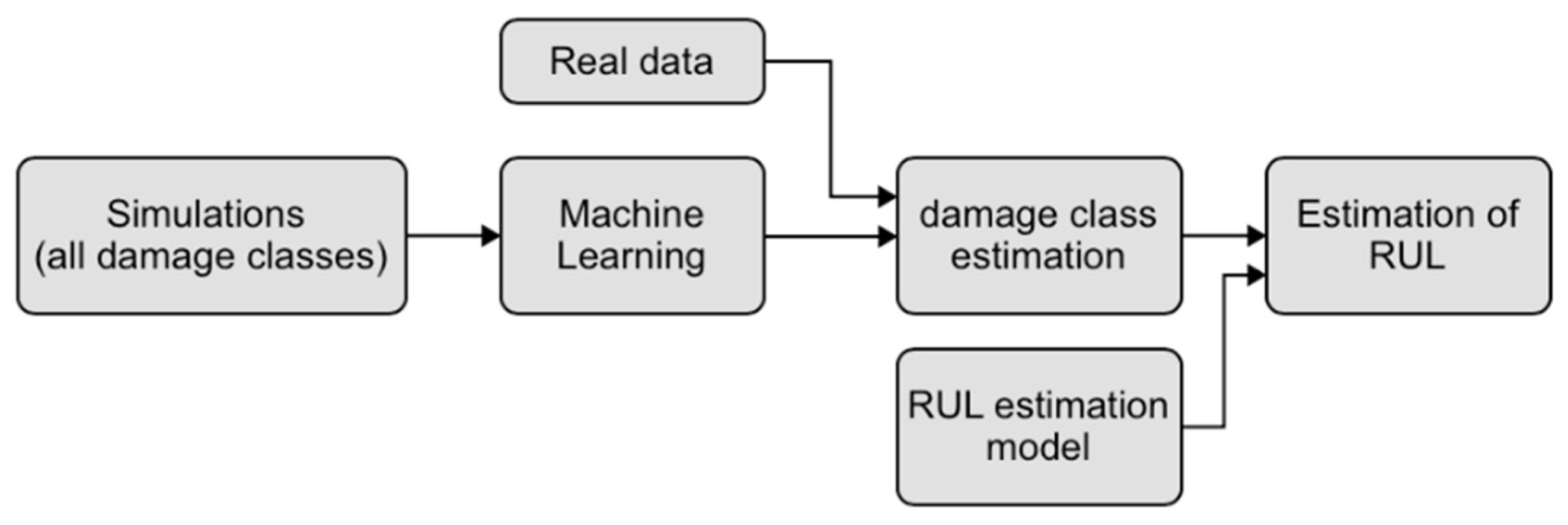
This section describes the methodology used in this article. One of the main aspects for the application of this framework is the creation of a database of signals that includes the response of the studied structure in different damage configurations. Since it is not possible to obtain such a database through actual records, a parametric FE model is analyzed. Starting from this database, it is possible to continue the AI training with supervised ML techniques, since the signals are labeled. At this point, the second part of the work focuses on the estimation of RUL, i.e., by recording the real signals and by identifying the class of current and past damage, it is possible to estimate the RUL through a degradation mathematical model. Since it is not possible to have real data available, the previous model was considered and modified to simulate the progression of damage (in this case, uniform corrosion on the reference steel column) over time. Figure 1 shows the general framework just described.
In this work, only the damage associated with a uniform corrosion pattern was considered, without taking into account the influence of environmental variables on the extracted features, such as temperature, humidity, wind load, and others. The only random variable considered is the mass acting on the steel column. It is plausible that if the method can identify the damage despite the noise due to mass variations, it will also be possible to identify the damage in the case of simultaneous environmental variables. In addition, the specification of a uniform corrosion pattern could be considered a limitation. However, the objective of this article is not to study the corrosion phenomenon in depth, but to develop a framework for damage identification. Therefore, corrosion was used here as a degradation phenomenon to test the damage progression identification framework.
3. Damage Detection Using Machine Learning Techniques
This section highlights an approach to monitor and detect damage using ML techniques. In the context in which we work, SHM means training an AI to associate a state or class of damage with a vector of measurements of the structure of interest. The vectors of measurements should consist of quantities, i.e., features, which are sensitive to the type of damage being studied. The features could be, for example, the first identified fundamental frequencies of vibration, statistical parameters of the recorded signal, wavelet coefficients, or artificial scalar quantities computed from seismic signals recorded at the structure, among others. Once the appropriate features are determined, which is not straightforward, a “map” between the features and the damage class of the structure can be created to extract mathematical models that can automate the SHM process and eliminate the intervention of human technicians as much as possible. The goal of SHM is to gather enough information to take appropriate corrective and preventive actions to restore and preserve the artifact, or at least to ensure its safety.
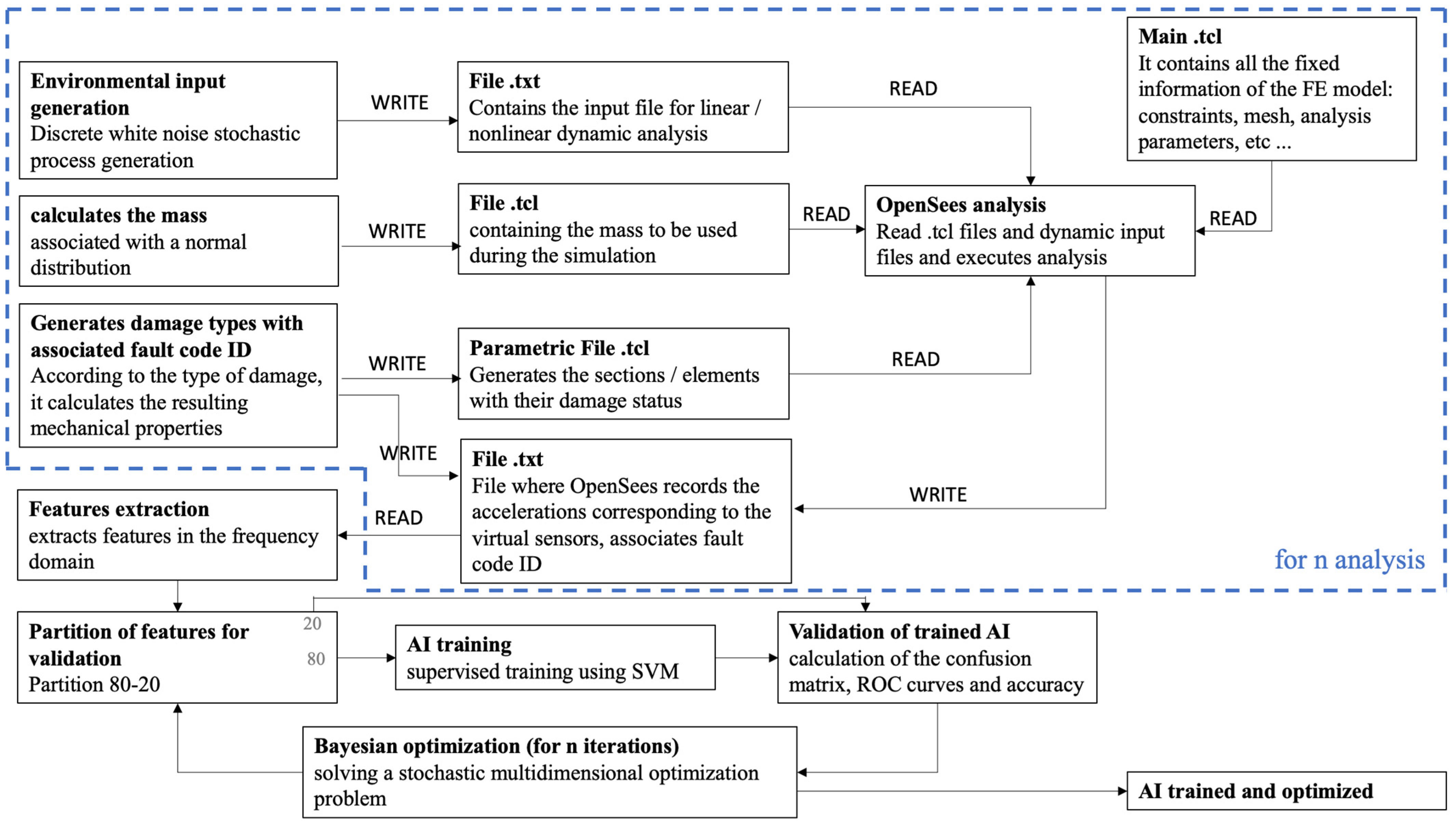
The approach discussed here for solving the classification level is based on the idea of pattern recognition (PR). In a general sense, a PR algorithm is simply an algorithm that assigns a label, a class label, to a sample of measurement data. The class labels encode the location and rating of the damage. The training method, in which the diagnosis is trained by linking labels and a full set of measurement data (including those of the different damage classes), is called supervised learning. A supervised learning approach, unlike unsupervised learning, imposes very stringent requirements on the data needed for learning. First, as described earlier, measurement data are needed for every possible damage configuration, and such data are difficult to find in the civilian domain. One option would be physical FE modeling. However, FE modeling could be hampered by several problems, such as: the a priori choice of the damage type, and the model could be complex in geometry and material definition and, therefore, the analysis could take a lot of time. Moreover, it could be difficult to model the damage accurately, especially in the case of nonlinearities or in the case of fatigue cracks with cyclic opening–closing phenomena. Finally, there are uncertainties about present and future loading and environmental conditions. An alternative solution could be to make small-scale or full-scale copies and then damage them. the number of copies should correspond to the combination of the different types of damage that can be assumed based on their varying severity. However, this solution is simply not feasible for construction works. The proposed framework is shown schematically in Figure 2. Briefly, the framework uses a parametric FE model (here using the FE software OpenSees [26]) for damage definition and stochastic variables for environmental conditions. The FE model is used to train a ML model, using the SVM method. Details are provided in the following sections.
4. Support Vector Machine (SVM)
Once the features have been extracted, it is possible to proceed with the AI training. In this case, it was decided to use a supervised learning approach using SVM [27,28,29,30,31,32,33]. SVM belongs to a class of ML algorithms called kernel methods or kernel machines (here, we considered Gaussian, linear, and polynomial kernels). Before training the actual classifiers, we need to divide the data into a training set and a validation set. The validation set is used to measure accuracy during model development. A SVM constructs an optimal hyperplane (by solving a quadratic optimization problem) as a decision surface to maximize the separation distance between two classes. The support vectors refer to a small subset of the training observations that are used as support for the optimal position of the decision surface.
Only the support vectors selected from the training data are needed to construct the decision surfaces. Once the decision surfaces are identified, the remaining training data are not considered.
5. Case Study
5.1. FE Model
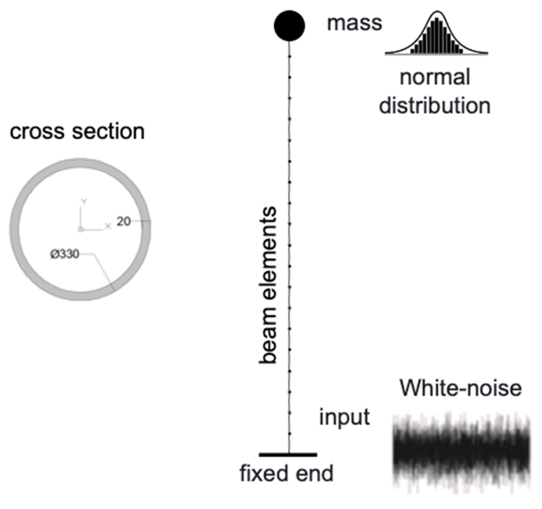
A simple cantilever column embedded at the base and supporting a vertical load and mass at the top was selected to test the concept. The column is 6 m high and has a circular–pipe cross-section with an outer diameter of 330 mm and a thickness of 20 mm. The damage was simulated simply as a uniform, general reduction in thickness due to corrosion, without capturing the electrochemical corrosion process. The structure type and geometry could be related to columns of industrial buildings, residential buildings, bridges, and wind turbines. The column was modeled by 20 beam elements (Figure 3). All the information, such as input, mass, and damage conditions, are generated in the MATLAB environment and then input into OpenSees [26] to perform the actual analysis. Once the synthetic signals are computed, they are brought back into MATLAB for further processing.
The case study presented here allows us to test the framework for damage detection and subsequent estimation of the remaining useful life after a simulated corrosion process. However, the case study is intended as a benchmark for any type of degradation/damage.
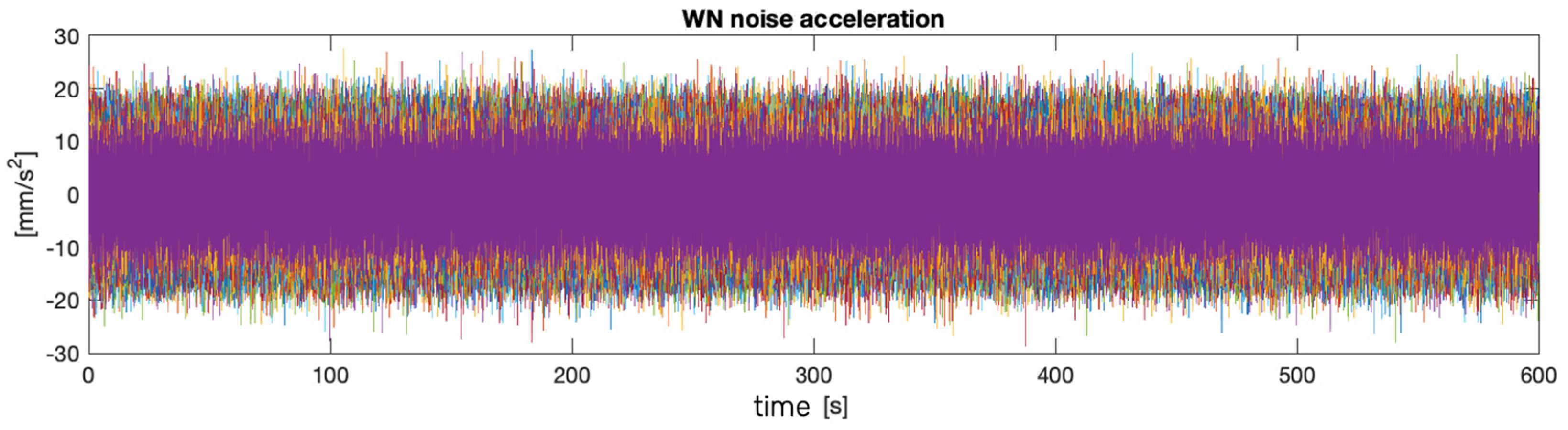
The external loading condition is characterized by an ambient vibration at the base, representing a stochastic Gaussian white noise process. Sixty synthetic signals were defined (Figure 4).
5.2. Feature Extraction
A series of response history dynamic analyses is performed to obtain the structural vibrations in terms of the acceleration time history of the top of the column (since it is basically a 1 degree of freedom, DOF, system). Then, these signals are analyzed and processed to extract features (usually scalar quantities) that can quantify the health of the structure. These features can be extracted either in the time domain or in the frequency domain. The features analyzed are reported below. Each time series is stored with a health code that is later used for artificial intelligence (AI) training.
In this paper, the following features are extracted and analyzed:
- peak amplitude
- peak frequency
- damping coefficient
- peak band
- natural frequency
For dynamic identification, the frequency domain decomposition (FDD) algorithm [34] is used, where the search for the resonance peaks is automated using a local maximum search algorithm.
Once the features were extracted, they were plotted on graphs so that their quality could be quantified. An excellent feature allows easy discrimination of the healthy or unhealthy state of the structure. The algorithm, one-way analysis of variance (ANOVA), was used to quantify the goodness-of-fit of the extracted features. This is to determine if the data from different groups have a common mean. ANOVA thus makes it possible to find out if different groups of an independent variable have different effects on the response variable. The one-way ANOVA is a simple case of a linear model. Such a model has the form:
where:
is an observation: i represents the observation number, and j represents a different group of the predictor variables y;
represents the population mean for the j–th group;
is the random error, independent and having a normal distribution with zero mean and constant variance .
ANOVA assumes that all distributions are normal or with small deviations from this assumption. In this study, this assumption is satisfied.
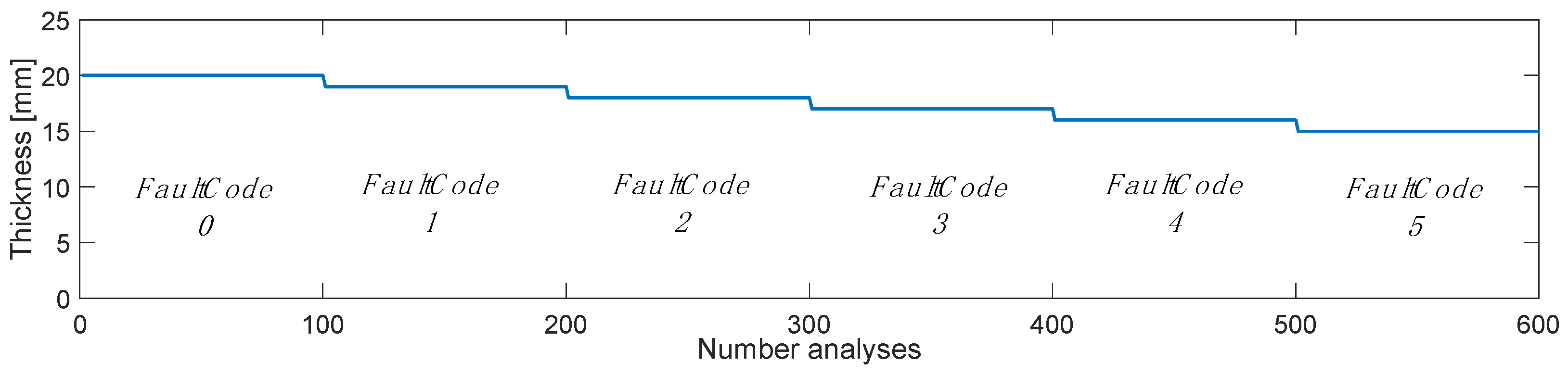
In this section, we examine how the AI responds to training, including damage with multiple classes. Specifically, the goal is to predict a corrosion thickness with a sensitivity of 1 mm and a maximum of 5 mm. Figure 5 shows the training scheme used; 600 response history analyses were performed by integrating as many stochastic white noise processes, where 1 mm of thickness is removed every 100 analyses to simulate the layer lost to corrosion. FaultCode 0 corresponds to the healthy state, while from FaultCode 1, the removal of 1 mm of thickness was started; in this way, the FaultCode identifier also corresponds to mm of corrosion loss.
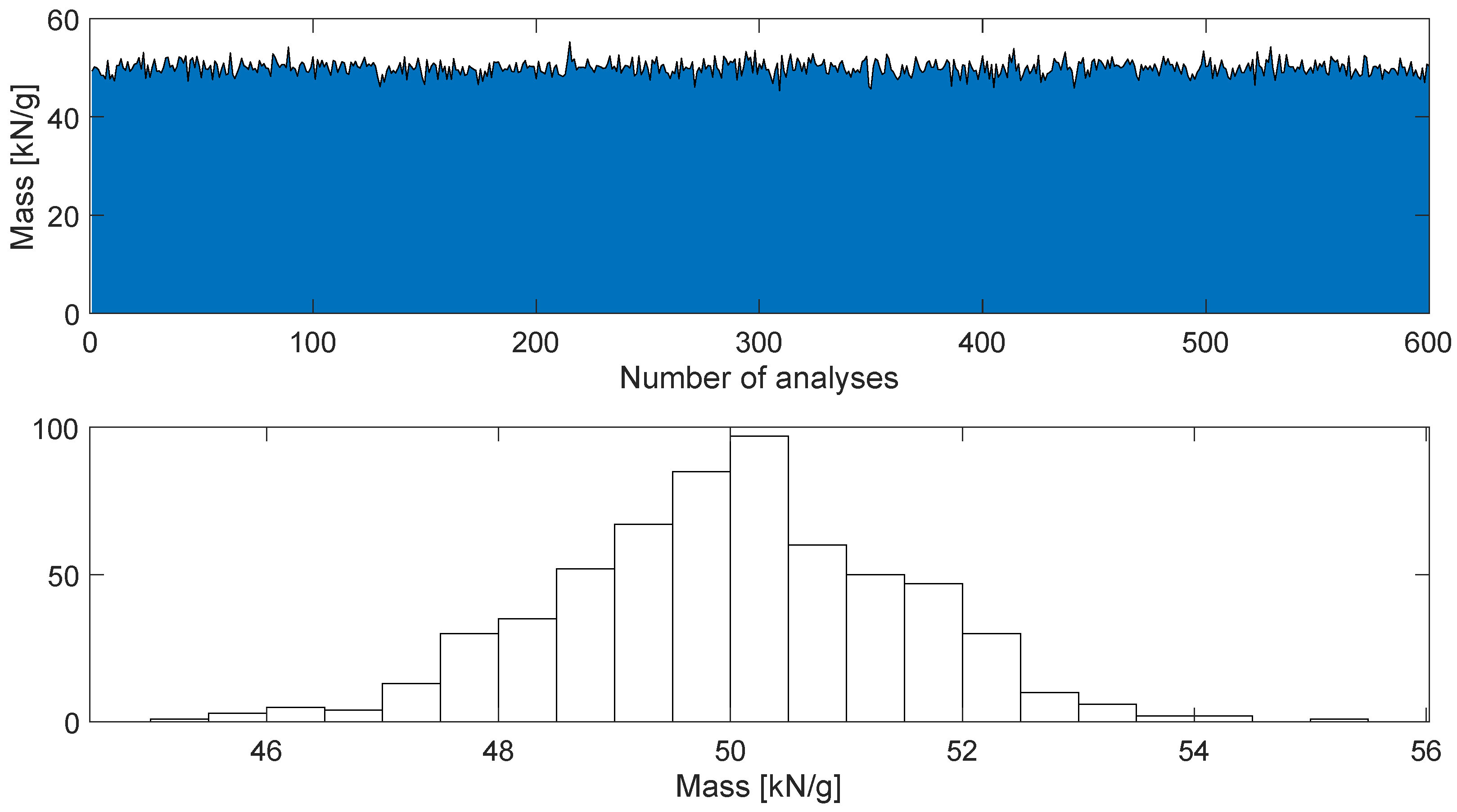
To best simulate the typical conditions of a structure, the mass lumped at the top of the column was introduced stochastically (while it was kept constant in the single analysis to keep the mass assumptions invariant during the i–th record). A plot of the introduced mass change is shown in Figure 6. This condition represents a challenge for AI prediction, as the AI must distinguish and recognize the change in features due to a change in stiffness (in this case due to corrosion) from a change in mass.
Experience and testing have shown that even training AI with the same parameters and features results in different AI with different performance. Therefore, the question arises: what are the parameters that can best be used to train AI with the same features?
An optimization problem is then configured for the AI training parameters, properly called hyperparameters hereafter, with the goal of minimizing the error function in classification. The problem takes the form of a huge and incredibly complex multidimensional optimization problem, and it also has a stochastic objective function, since the outcome varies each time an AI is re–trained with the same parameters. This problem cannot be addressed with classical deterministic optimization algorithms. In this work, Bayesian optimization is used.
5.3. Bayesian Optimization
The adopted Bayesian optimization internally manages a Gaussian process model (GP) of the objective function and uses evaluations of the function itself to train the model. Bayesian optimization uses an acquisition function, which the algorithm uses to determine the next point to evaluate. The acquisition function can compensate for sampling at unexplored points or explore areas that have not yet been modeled [35]. A summary of the actual treatment of this technique can be found here. The Bayesian optimization algorithm attempts to minimize an objective function in a finite domain. The function can be deterministic or stochastic (as assumed in this research), which means that it can give different results when evaluated at the same point.
The key elements of the process are:
- a Gaussian process of [36]
- a Bayesian updating procedure to change the GP with each new evaluation of
- an acquisition function (based on the GP model of ) that is maximized to determine the next point of for the evaluation of the objective function
- an evaluation of for randomly taken points of within the limits of the variables
- an update of the GP of to obtain a posterior distribution
- a definition of the new point that maximizes the acquisition function on
6. Results
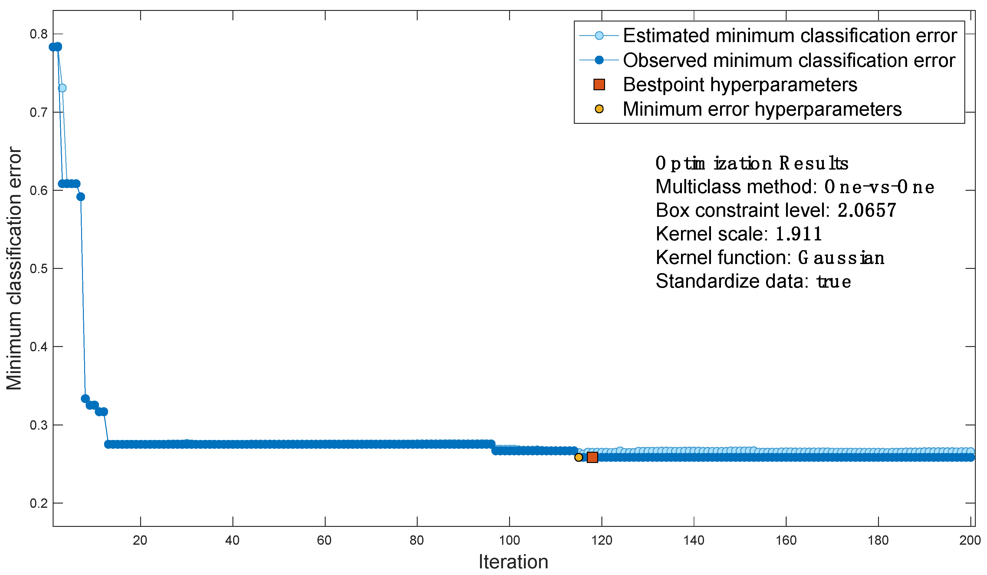
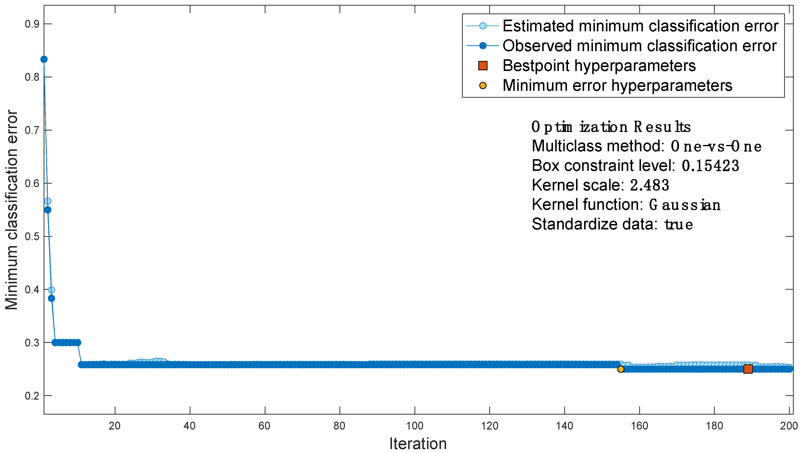
For the case study considered, the classification error function is shown in Figure 7, which contains the output of Bayesian optimization:
- each blue dot corresponds to an estimate of the minimum classification error computed by the optimization process when all sets of hyperparameter values tested so far, including the current iteration, are considered. The estimate is based on an upper confidence interval of the current classification error objective model.
- Each dark blue dot corresponds to the minimum observed classification error computed so far by the optimization process.
- The red square indicates the iteration corresponding to optimized hyperparameters. Such hyperparameters do not always yield the minimum observed classification error. Bayesian hyperparameter optimization chooses the set of hyperparameters that minimizes a higher confidence interval of the objective model of the classification error, rather than the set that minimizes the classification error.
- The yellow dot indicates the iteration corresponding to the hyperparameters that yield the lowest observed classification error.
Then, the best point is extracted as the optimized AI.
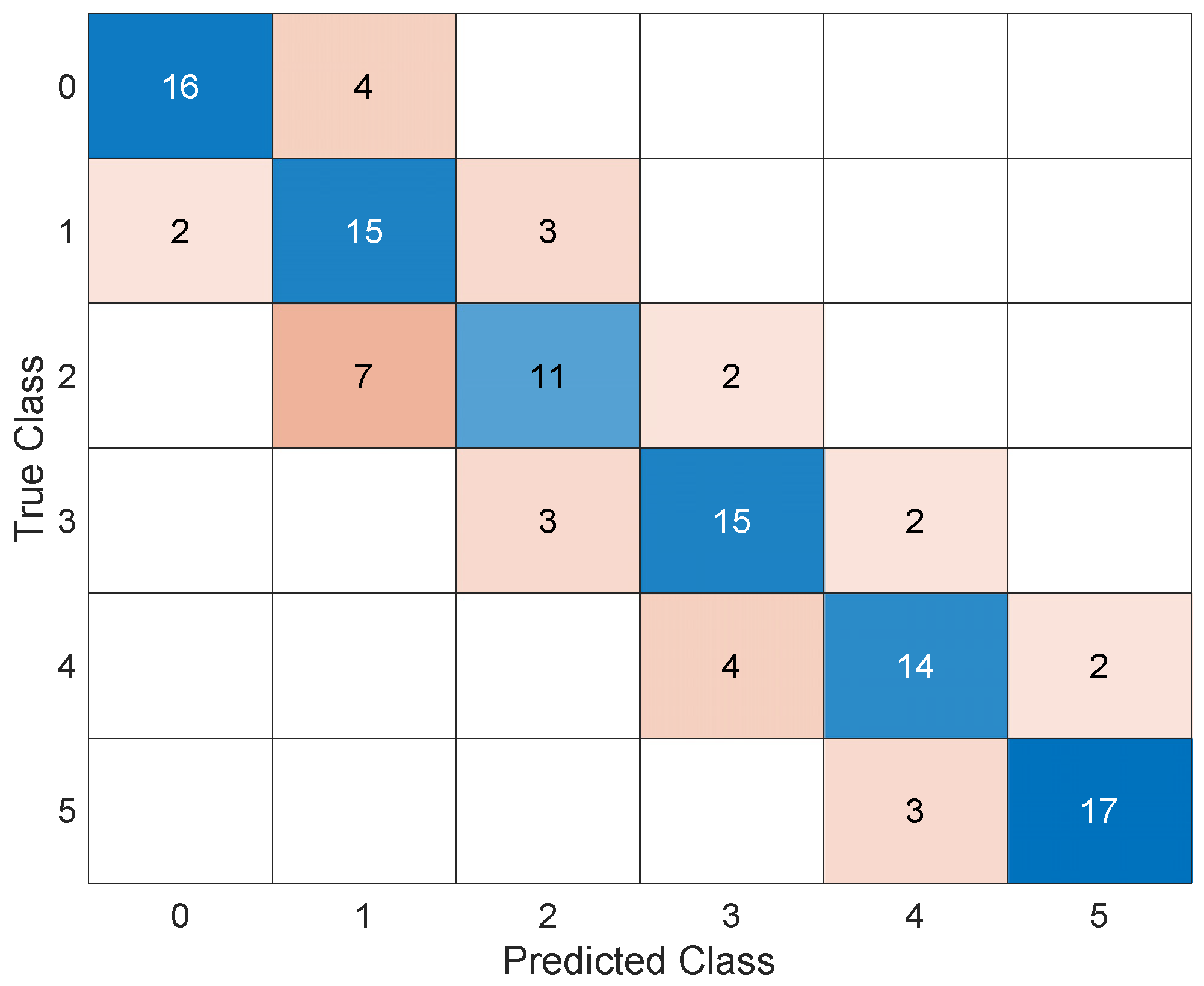
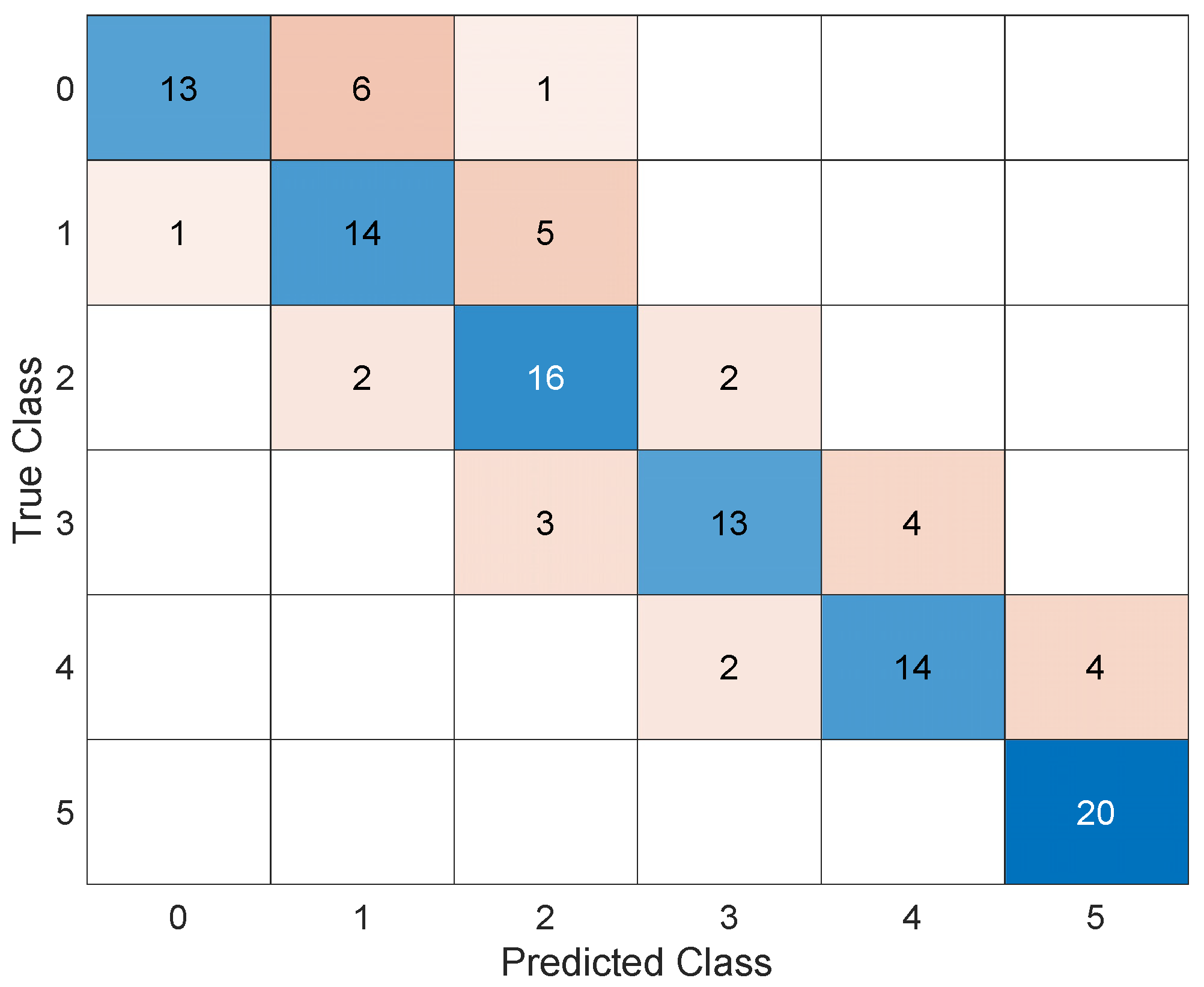
For sake of brevity, the results of this AI in the form of scatter plots, parallel plots, and ROC curves are omitted; instead, the corresponding confusion matrix after validation is shown in Figure 8. The trained AI achieves an accuracy of 73.3 percent and commits a maximum error in estimating the corroded thickness of 1 mm.
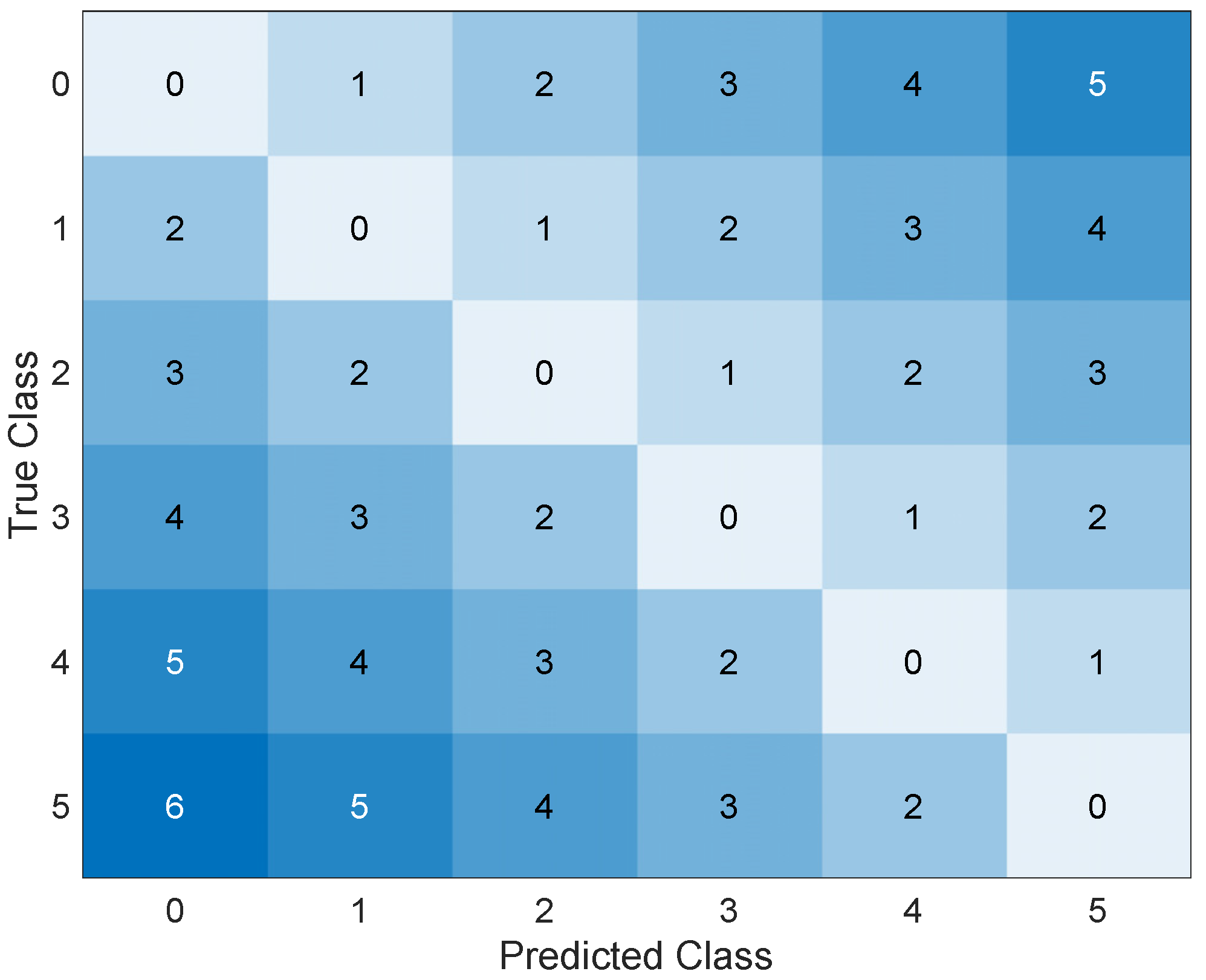
It is worth noting that a distinction should be made between the different types of errors: the error in the upper triangular matrix corresponds to an overestimation of the actual damage, which would lead to false alarms in real applications, while the errors in the lower triangular matrix are associated with an underestimation of the actual damage, which may lead to missed alarms. While these two types of errors are the same in terms of damage quantification, they can have very different consequences: a false alarm is costly because of the inconvenience it causes, while a missed alarm can jeopardize the safety of the work and people. Based on these considerations, it is interesting to define how to translate these technical observations so that AI can learn from them. The solution found is to insert penalties during the learning phase that limit the number of missed alarms in favor of false alarms. Figure 9 shows the penalty matrix used. Then, the AI was re–trained through optimization.
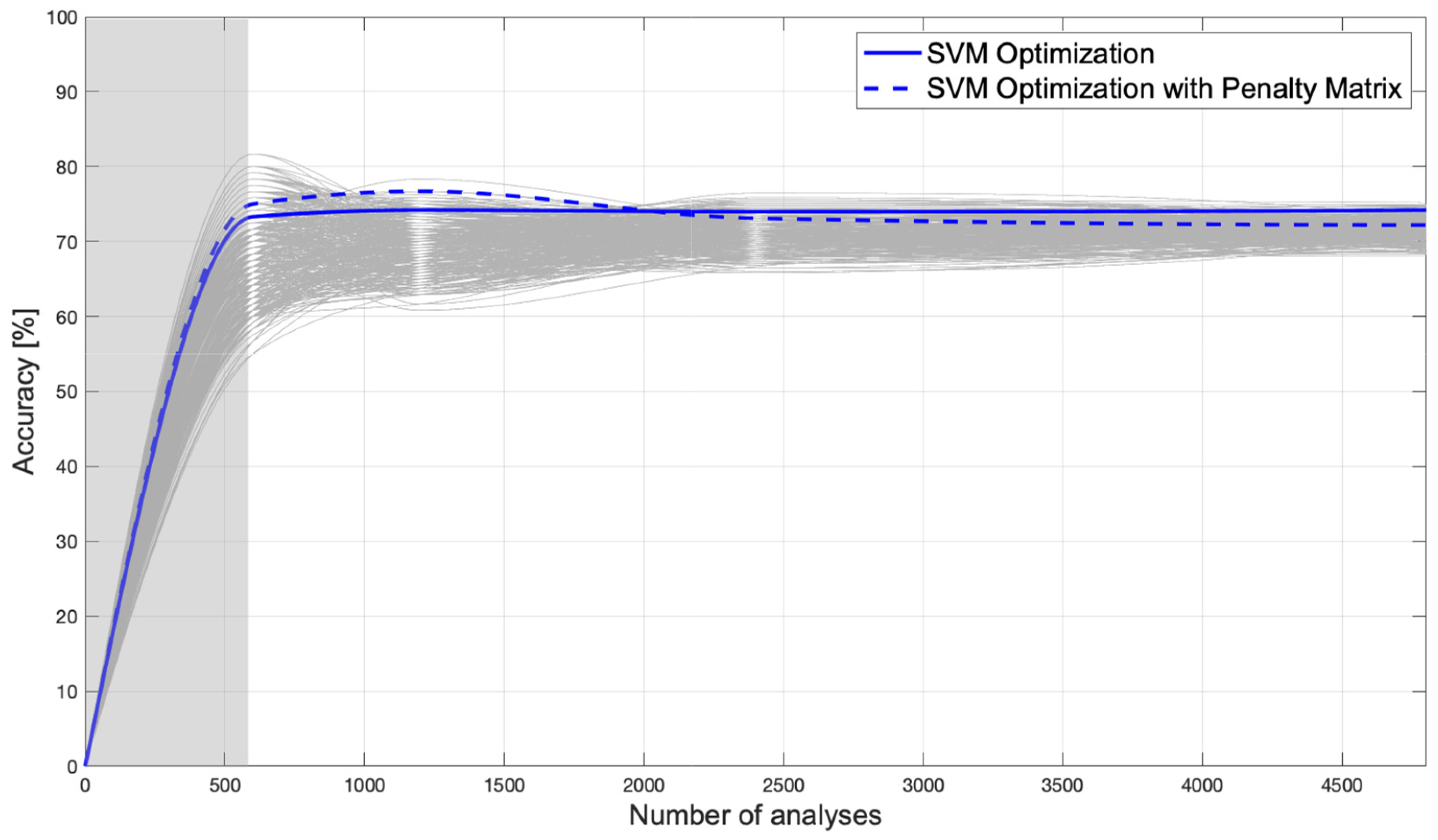
The resulting AI achieves an accuracy of 75.0% and commits a maximum error in estimating the corroded thickness of 1 mm. The introduction of the penalty matrix could also lead to a decrease in accuracy (although only to a very small extent) because its objective is not to increase accuracy, but to improve structural safety. Figure 10 and Figure 11 show the classification error function and the confusion matrix of the AI trained with the penalty matrix, respectively. Figure 12 shows how well Bayesian optimization fits. Nevertheless, Bayesian optimization succeeds in finding one of the best possible AIs, but not the absolute best, because AIs with higher accuracy can be seen from the figure. Thus, one could argue that Bayesian optimization allows one to find an excellent (not the best) AI without having to perform many iterations to understand its variability and then take its maximum; the solid blue line remains close to the upper bound. Figure 12 shows the accuracies obtained by training tens of thousands of AIs trained by hyperparameter randomization. The accuracy of a Bayesian optimized AI with an additional penalty matrix is shown in the dashed blue line; the resulting accuracy is very similar to that without a penalty matrix. As mentioned earlier, this is not a problem, since the goal is to reduce the probability of missed alarms. We also wanted to use this plot to examine the variability in accuracy as the number of FE analyses performed for training changes. Specifically, we started with 600 training analyses and increased the number to 4800. It can be seen that the variability of accuracy decreases as the number of analyses performed increases, and there is no overfitting.
7. Remaining Useful Life Estimate
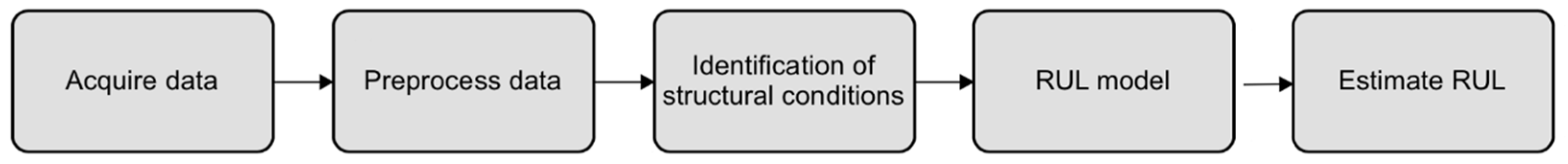
Predictive maintenance is a maintenance approach that uses predictive mathematical–statistical models, typically based on data recorded by sensors, to detect anomalies, identify the quantity and quality of damage/degradation, and estimate the remaining useful life (RUL). Figure 13 shows a simple flowchart for RUL estimation.
In Figure 13, the first step is to collect data from the monitored system. Then, the raw data are pre–processed to feed into a damage detection algorithm (this step can be based on ML, among others). In this step, different techniques can be implemented, both traditional and AI techniques, to detect anomalies, classify the type of anomalies or damage, quantify and localize the damage, and estimate the remaining lifetime of the structure. It is advantageous to collect as large and heterogeneous a dataset as possible. This is achieved by collecting data under different operating conditions, such as environmental conditions, which allows the development of a more robust algorithm. In civil engineering, representative damage data are hardly available. Therefore, a mathematical model can be developed to predict system response as a function of parameters and environmental conditions.
Such response signals are called synthetic signals and should be integrated with the recorded data of the real structure. When the desired amount of real data is not available, integration between real data (undamaged structure) and simulated data (damaged structure) is generally sought. The real data are affected by measurement errors due to the measurement infrastructure, while the simulated data are affected by model errors due to simplifications in the mathematical description of the physical phenomenon. Once the data are recorded or simulated, the next step (Figure 13) is to preprocess them to facilitate the identification of health indicators. This step could be based on one or more techniques, such as noise removal, outlier elimination, dummy trend elimination, frequency domain transformation, and many others. The next step is to identify the structural health by calculating and comparing features that respond to the type of degradation/damage analyzed. These features are used to distinguish a healthy operation from a damaged one. In the present work, the last and the previous steps are performed by applying AI. Finally, the last two steps in Figure 13 define a relationship between the health status estimated by the AI and the aging path of the structure, by allowing one to estimate the remaining useful life (RUL) for the structure by imposing a minimum safety threshold and, thus, defining maintenance schedules.
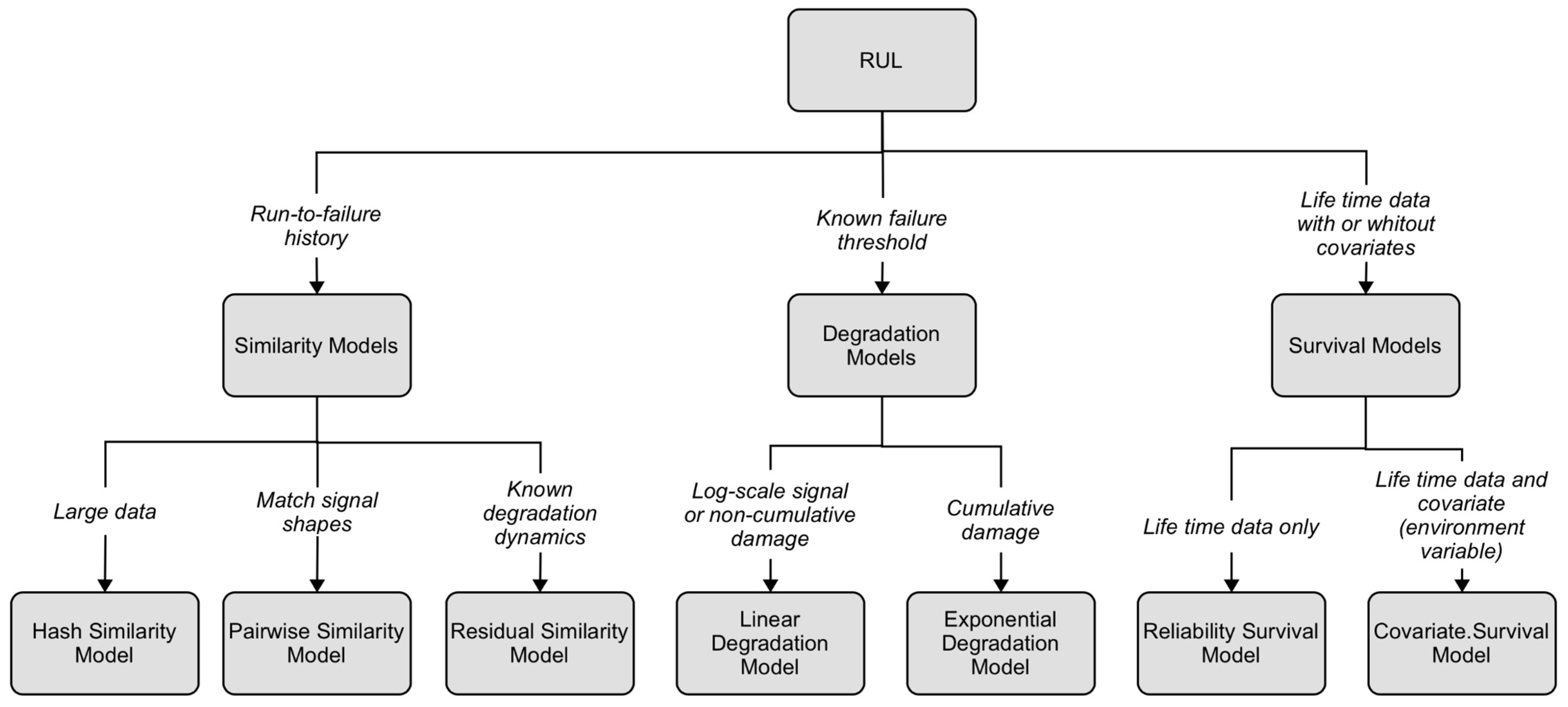
The RUL is defined as the time between the current situation and the minimum performance threshold established for the structural system. Depending on the situation, the time may be expressed in days, flights, cycles, among others. For civil engineering works, the RUL is specified in years. Algorithms for RUL calculation can be divided into three categories: similarity algorithms, survival algorithms, and degradation algorithms. Figure 14 shows the different methods for calculating RUL. The choice of the most effective method depends on the system and the available data. The degradation model method is used when undamaged state data are available and a safe threshold can be defined. It is possible to use this information to update a mathematical model of degradation to a performance indicator and then use the history recorded up to that point to predict how the indicator will change in the future. In this way, it is possible to statistically estimate the remaining time before the indicator reaches the imposed threshold and, thus, the RUL. A linear degradation model can be used for this purpose if the system does not experience cumulative degradation. The mathematical model describes the physical process of degradation as a stochastic linear process. If, on the other hand, the system experiences cumulative degradation, an exponential degradation model is used, in which the physical process of degradation is modeled by an exponential stochastic process.
For civil engineering applications, the best models for RUL estimation are degradation models (i.e., models in which the failure threshold is known, Figure 14). Other types of models (i.e., similarity models and survival models, Figure 14) were initially discarded because structural and infrastructure works are typically unique, thus it is difficult to have the required data for the operating conditions, including degradation data. These models require as input a single health indicator, which, herein, is derived from the raw data obtained from the AI model, i.e., the estimated corrosion thickness, as indicated in the previous section. The degradation models used herein is the exponential model, which implements a stochastic model with an exponential degradation over time [41,42,43,44,45,46,47,48]:
where:
is the intercept of the mathematical model at the origin
is a random variable modeled with Lognormal distribution
is a random variable modeled with Gaussian distribution
is the model noise implemented as a random variable with normal distribution
is the variance of the noise
8. Case Study Application
The cantilever steel column considered before is analyzed with some modifications to test the RUL calculation. First, the damage of the column (i.e., the corrosion thickness) was correlated with time, assuming a continuous degradation rate equal to 80 micrometers/year, which is the reduction associated with an urban–industrial environment [49].
Figure 15 shows the framework developed and implemented. Herein, the gray-highlighted portion allows creating benchmark data to test the RUL algorithm. The whole framework is repeated whenever the damage evaluation is required, thus allowing the update of the parameters of the degradation model. As shown in Figure 15, the approach is very similar to the AI training described in the previous section. The lumped mass at the top of the column was introduced in stochastic terms, the signal at the base was reassigned in each iteration as a pseudo–random white–noise signal to simulate environmental vibrations, and the damage parameterization was modified to account for a time–dependent damage function (in this case a function governing the corrosion rate).
The following parameters have been used:
- corrosion rate: 80 micrometers/year
- simulated operating period: 60 years
- number of damage estimations for each simulated year (i.e., number of runs of the trained AI to estimate the corroded thickness): 10
- input signal: pseudo–random white noise signal, with a length of 10 min and a sampling frequency of 200 Hz, for each damage identification run
- safety threshold: 5 mm of corroded thickness
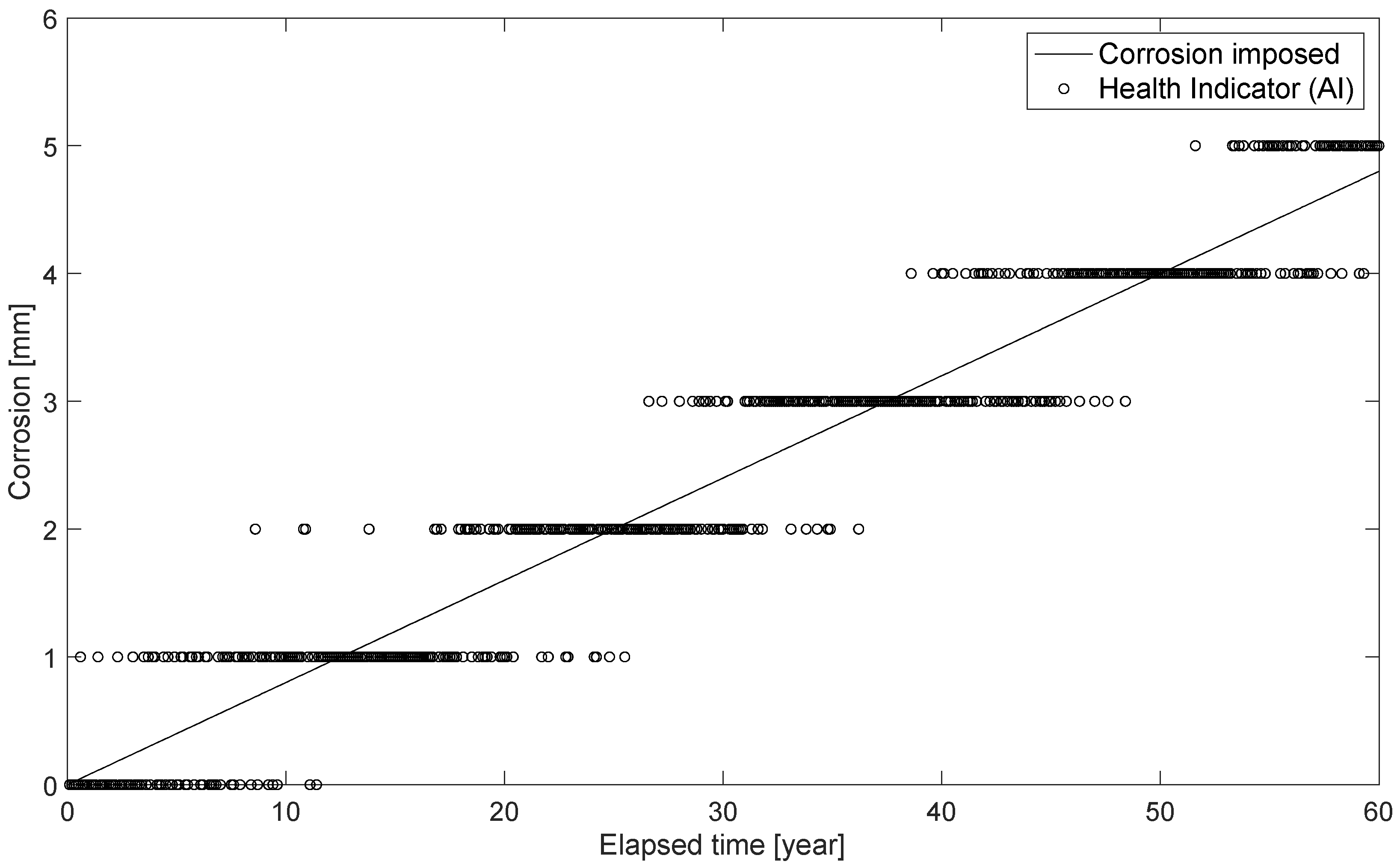
Figure 16 shows the comparison between the thickness lost in the corrosion process associated with the assumed corrosion rate, i.e., the thickness reduction entered in the FE model, as well as the AI prediction. The discontinuity of the latter is due to the AI training phase, where the recognition of a corrosion thickness with a sensitivity of 1mm was set. One could have opted to create a training scheme with higher sensitivity, say 0.5 mm, in the training phase. However, this would certainly have lowered the accuracy, as the AI would have struggled more to recognize a smaller variation in the extracted features (e.g., natural frequency). The number of analyses to be performed is another important aspect affecting the choice of the training scheme. As mentioned before, seeking a more sensitive and accurate AI results in an increase in the number of signals to be created, which may be far from negligible. Herein, the proposed AI represents a good compromise between training time, sensitivity, and accuracy, even if it sets up a discontinuous trend. The best compromise between computational time and sensitivity will be the object of future developments.
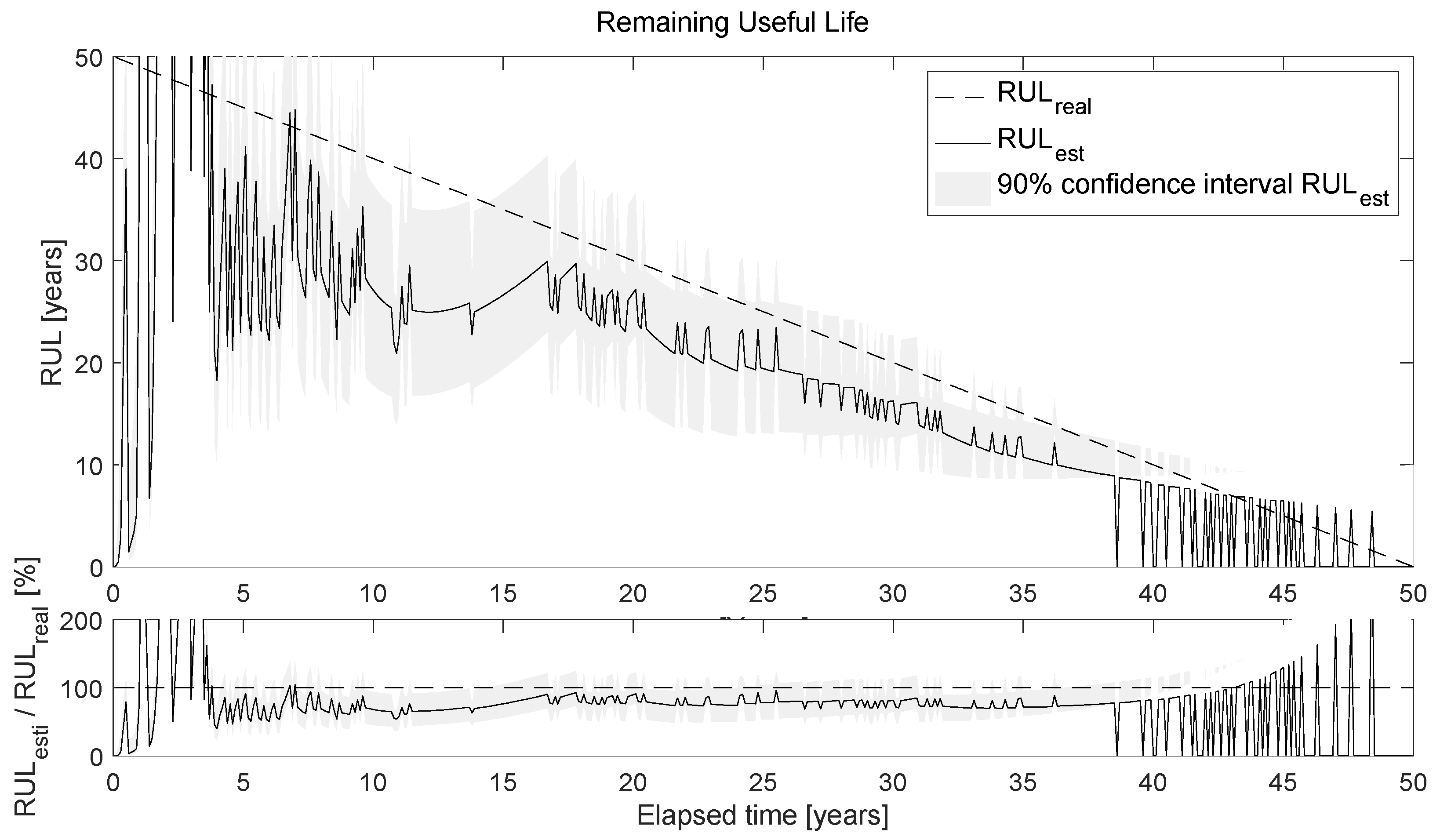
Figure 17 shows the output of the RUL algorithm (Figure 15). The algorithm is run for each new identification, and at each time point, the RUL is recalculated by updating the parameters. The diagram above shows the comparison between the real RUL (RULreal), i.e., the remaining useful life calculated by knowing the confidence limit (5 mm of corrosion) and the corrosion rate function, as well as the RUL obtained by updating the degradation model (RULest). The confidence interval of the latter is also given. The bottom graph shows the ratio RULest/RULreal in percent.
One important aspect immediately stands out: the estimated RUL almost overlaps with the actual RUL in the period between about 15 and 40 years. This proves the excellent estimation of the forecast. In contrast, the estimation before 10 to 15 years and after 40 years is unreliable, but not problematic, if we consider the nature of the phenomenon: in the early years of the structure’s life, the algorithm will learn and update itself to detect the physiological degradation trend of the structure (of course, in the case of damage/pathological degradation, there is always an AI that can provide us with a snapshot of the current damage state), and, in this time frame, it is less relevant to estimate the RUL; analogously, in the last moments of the structure life, it is obviously useless to estimate the RUL, since the damage identification AI will report damage close to the imposed threshold. Instead, in the intermediate life span, it is important to make an accurate RUL estimate in order to detect and locate future damage and have enough time to effectively plan maintenance actions.
However, it is interesting to note that the estimated RUL is practically always lower than the actual RUL, i.e., it underestimates the actual RUL. From a structural safety perspective, it is certainly better to be in this state than in the opposite state, i.e., overestimating the RUL. From a mathematical point of view, this is due to two factors: the degradation model used is exponential, and a penalty matrix was used in the AI training. The exponential degradation model, even if updated, will always provide a shorter remaining life than a linear degradation model due to its curvature. From the authors’ point of view, it is not recommended to use a linear model: first, because underestimating the RUL is beneficial for structural safety, and second, because it is not possible to know the shape of the degradation function a priori. Thus, if we use a linear degradation model and the degradation function turns out to be exponential, we would overestimate the RUL to the detriment of safety. At the same time, the introduction of the penalty matrix in the AI training phase leads to a higher probability of overestimating damage, which in turn leads to an underestimation of the RUL.
One aspect that could have a strong impact on RUL is the discontinuity of the damage estimated by the AI, as shown and discussed in Figure 16, due to the solution of a classification problem. Future developments in this regard could include methods to reduce the discontinuity of damage estimation so that a more faithful reconstruction of the degradation history is available. Another solution could be to implement techniques for interpolating or averaging the damage classes resulting from AI to facilitate the RUL update algorithm.
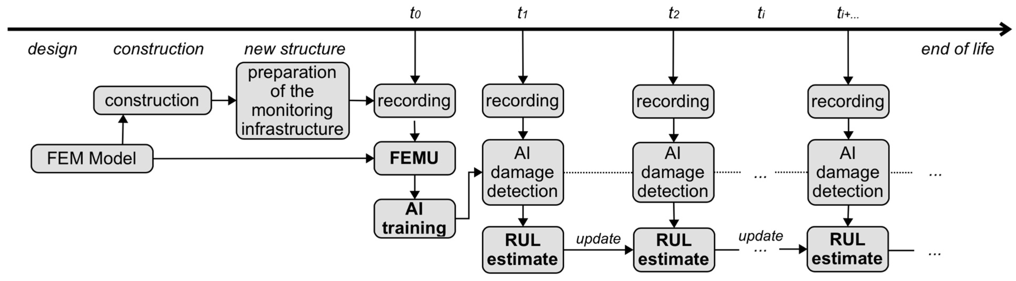
A hypothesis on the possible use of RUL calculation throughout the life cycle of the structure is presented in Figure 18. All the techniques developed and presented in this paper are designed for estimating the remaining useful life. Once the construction of the structure is completed and the monitoring infrastructure is properly installed, it is possible to update the FE model based on the recorded data (FE model, which could end up being the same model used for the design of the structure). In this way, we obtain the FE model needed for the AI training. This FE model will undoubtedly be more accurate than an outdated model as a result of the optimization problem. In this way, we will minimize the model error in the AI that will be trained with the signals derived from this FE model. Once the training phase is complete, we will have an AI that can estimate the damage (with some accuracy and therefore uncertainty in the estimate) and we can use this information as input for estimating the remaining useful life. At this point, every time we perform a registration, we will estimate the damage over the previously trained AI and iteratively update the RUL calculation.
Finally, the possibility of extending the proposed framework to real structures involves additional considerations. First, the effects of environmental conditions may challenge feature extraction compared to synthetic signals. Second, the measured data will be affected by measurement errors due to the accuracy of the sensor. This could affect the goodness of the proposed features and, if this goodness is compromised, new features must be defined, or the existing ones must be improved. In fact, this is not a major problem if high-performance sensors, measurement systems and data transmission infrastructures that are used. Assuming that this framework is widely used, one would need to address the computational power required for AI training, especially with respect to the creation of the various synthetic signals through dynamic FE analysis, which is the real bottleneck of the whole process. Assuming that the random and parametric training in Figure 12, which was performed for research purposes and to understand the effectiveness of Bayesian optimization, should be avoided and, instead, once the signals are generated, we should proceed with the training through hyperparameter optimization, the question arises as to how much computational power or how much time is required to generate signals of a structure with multiple types of damage and different severity levels. As a simplified estimate, we can easily determine the number of analyses and thus the computational time required.
Indeed, it is possible to calculate the total computational time with the following formula:
where:
TT represents the total time to create the synthetic signals
SAT represents the time to perform a single analysis with the FE model
NAID represents the number of analyses to be performed for the same damage configuration to account for the variability of stochastic parameters
is the number of the arrangements with repetition where: n is the number of damage severities and k is the number of the different types of damage to be investigated
When calculating analysis time for real-world use cases, it is possible to see how much time is required for complex civil structures that easily reaches the order of hundreds, if not thousands, of years. However, this is where methods to increase computational power, such as parallel computing and cloud computing, come to the rescue. With these techniques, it is possible to divide a large problem into smaller problems that can be developed and solved in parallel. In fact, these techniques are easy to implement in the proposed framework, since each analysis is independent of the others. Even if, at first sight, the results just reported give the impression that the application of this methodology is difficult, it is necessary to consider the various advantages that can be obtained.
9. Conclusions
This paper proposed and investigated a framework for estimating structural damage using machine learning techniques (ML) and the resulting remaining and useful life (RUL). The applied ML technique involves supervised training, so knowledge of the data for the undamaged and especially for the damaged structural system is required. Considering the uniqueness of civil structural systems, training data for the different damage classes are not available. Therefore, a hybrid-based approach was adopted here: a FE model is used as a digital twin to generate synthetic damage data. The proposed, implemented, and numerically tested framework seems to be able to estimate, quantify, and localize the damage (in this case the corrosion thickness of a reference steel column) in a robust, reliable way and with very good accuracy.
A reliable estimate of actual damage is a necessary prerequisite for RUL assessment. In this context, a framework for updating the RUL of a structural system has been proposed and investigated. To achieve this, a Bayesian approach is adopted for updating the parameters of the chosen exponential degradation model with random coefficients. After updating the degradation model, it is possible to determine the updated a posteriori distribution of RUL of the structure. Finally, the framework was numerically applied to the reference case study, with the trained AI serving as the basis for the probabilistic estimation of the current state of health.
The main scientific contributions in this research are the development of an innovative framework that allows a damage estimation AI to interoperate with the probabilistic RUL estimation model. The application of the framework to a numerical, albeit simple, structural system allowed validating the soundness of the method. Therefore, the added value of performing a Bayesian update of the parameters to properly incorporate the information into the RUL estimation model is significant.
In solving a supervised learning problem, such as the one presented in this paper, a fundamental and crucial aspect becomes clear: do we have data about the damaged structure (for all types and severities of damage)? If the answer is no, which is usually the case, one needs to find a way to estimate it. In this paper, we attempted to solve a supervised learning problem by developing a general framework that uses numerical FE modeling to produce synthetic data of the monitored structure. Of course, these data will be affected by model errors due to the various assumptions made in the development of the model itself. For this reason, we refer to this technique as hybrid-based: an AI model is created from the data all or part of which can be artificially generated by numerical simulations. To limit, but not to eliminate model errors, finite element model update (FEMU) techniques can be used to update the FE model before generating the synthetic data. In this way, model errors are minimized for a newly built structure, but, more importantly, the developed ML method could be used to monitor existing structures, thus already showing some degradation (whether physiological or pathological), in which case it would be strongly discouraged to proceed with AI training with a model representing the undamaged structure.
Another important point to consider when monitoring a structural system is its sensitivity to environmental conditions (e.g., temperature and humidity sensitivity, among others). Such conditions can cause features to change in a way that exceeds the change caused by potential damage. For civil engineering structures, such as bridges, mass can also have a significant effect on the modal properties of the infrastructure. Indeed, for these structures, variable loads and thus variable masses could be an important part of the loading on the whole structure. In the proposed framework, these random conditions are integrated into the mass parameter, which is randomly chosen and not included as a known parameter in the learning process. In this way, the AI is forced to distinguish a change in features due to uniform corrosion damage (i.e., a reduction in stiffness), as much as possible, from the change in features associated with random conditions.
Another aspect in favor of using techniques, such as the one presented here, is the possibility of in situ processing. Among other things, in situ processing has advantages in terms of speed of processing and reduction of the amount of data sent. Namely, while an enormous amount of computational time is required for training and especially for the creation of synthetic signals, the resulting AI after the training process, on the other hand, is very light and easy to process, even for very inexpensive CPUs. In summary, the use of this framework could lead to significant benefits in terms of accuracy and reliability of structure health estimations. Assuming that the development is extended to other types of materials and structures and tested in practice, the only limitation in its use could be the enormous computational cost. While on one hand, growth in available computational power is expected, it is undeniable how easy it is to configure an AI with a disproportionate need for signals. In this context, a simple equation has been reported that can be used to estimate the time required to generate the necessary synthetic data at a given power level. Alternatively, the required power (and, hence, the most appropriate engine) can be estimated as a function of the desired AI accuracy, which depends on the number of damage types and the number of damage severity levels selected.
Future research topics arising from these considerations could include improvement/refinement of the framework, numerical application to more complex structures, application to real structures that are also subject to changes in environmental conditions, and integration with decision models to determine the optimal timing for maintenance interventions.
Author Contributions
Conceptualization, S.C. and A.B.; methodology, S.C.; software, S.C.; validation, S.C. and A.B.; formal analysis, S.C.; writing—original draft preparation, S.C.; writing—review and editing, S.C. and A.B.; visualization, S.C. and A.B.; supervision, A.B. All authors have read and agreed to the published version of the manuscript.
Funding
This research received no external funding.
Institutional Review Board Statement
Not applicable.
Informed Consent Statement
Not applicable.
Data Availability Statement
Data are available upon a reasonable request.
Conflicts of Interest
The authors declare no conflict of interest.
References
- Farrar, C.; Worden, K. Structural Health Monitoring: A Machine Learning Perspective; John Wiley & Sons: Hoboken, NJ, USA, 2012. [Google Scholar]
- Worden, K.; Manson, G.; Fieller, N. Damage detection using outlier analysis. J. Sound Vib. 2000, 229, 647–667. [Google Scholar] [CrossRef]
- Figueiredo, E.; Park, G.; Farrar, C.; Worden, K.; Figueiras, J. Machine Learning algoritms for damage detection under operational and environmental variability. Strcutural Health Monit. 2011, 10, 559–572. [Google Scholar] [CrossRef]
- Zang, Y.; Burton, H.; Sun, H.; Shokrabadi, M. A machine learning framework for assessing post–earthquake structural safety. Struct. Saf. 2018, 72, 1–16. [Google Scholar] [CrossRef]
- Abdeljaber, O.; Avei, O.; Kiranyaz, S.; Gabbouj, M.; Inman, D.J. Real–time vibration based structural damage detection using one–dimensional convolution neurla network. J. Sound Vib. 2017, 388, 154–170. [Google Scholar] [CrossRef]
- HoThu, H.; Mita, A. Damage detection method using support vector machine and first three natural frequencies for shear structures. Open J. Civ. Eng. 2013, 3, 32514. [Google Scholar] [CrossRef] [Green Version]
- Mita, A.; Hagiware, H. Quantitative damage diagnosis of shear structures using support vector machine. J. Civ. Eng. 2003, 7, 683–689. [Google Scholar] [CrossRef]
- Gui, G.; Pan, H.; Lin, Y.; Yuan, Z. Data–driven support vector machine with optimization techniques for structural health monitoring and damage detection. J. Civ. Eng. 2017, 21, 523–534. [Google Scholar] [CrossRef]
- Chong, J.W.; Kim, Y.; Chon, K.H. Nonlinear multiclass support vector machine–based health monitoring system for buildings employing magnetorheological dampers. J. Intell. Mater. Syst. Struct. 2014, 25, 1456–1468. [Google Scholar] [CrossRef]
- Bornn, L.; Farrar, C.R.; Park, G.; Farinholt, K. Structural health monitoring with autoregressive support vector machine. J. Vib. Acoust. 2009, 131, 021004. [Google Scholar] [CrossRef] [Green Version]
- Kim, Y.; Chong, J.W.; Chin, K.H.; Kim, J. Wavelet–based AR–SVM for health monitoring of smart structures. Smart Mater. Struct. 2012, 22, 015003. [Google Scholar] [CrossRef]
- Sajedi, S.O.; Liang, X. A data framework for near reall–time and robust damage diagnosis of building structures. Struct. Control Health Monit. 2019, 27, e2488. [Google Scholar]
- Momeni, M.; Bedon, C.; Hadianfard, M.A.; Baghalani, A. An Efficient Reliability–Based Approch for Evaluation Safe Scaled Distance of Steel Columns under Dynamic Blast Loads. Buildings 2021, 11, 606. [Google Scholar] [CrossRef]
- Momeni, M.; Hadianfard, M.A.; Bedon, C.; Baghlani, A. Damage evaluation of H–section steel columns under impulsive blast loads via gene expression programming. Eng. Struct. 2020, 219, 110909. [Google Scholar] [CrossRef]
- Huang, M.; Gul, M.; Zhu, H. Vibration–based Structural Damage Identification under Varying Temperature Effects. J. Aerosp. Eng. 2018, 31, 04018014. [Google Scholar] [CrossRef]
- Huang, M.; Lei, Y.; Li, X.; Gu, J. Damage identificaiton of Bridge Structures Considering Temperature Variations–Based SVM and MFO. J. Aerosp. Eng. 2021, 34, 04020113. [Google Scholar] [CrossRef]
- Luo, j.; Huang, M.; Xiang, C.; Lei, Y. Bayesian damage identification based on autoregressive model and MH–PSO hybrid MCMC sampling method. J. Civ. Struct. Health Monit. 2022, 12, 361–390. [Google Scholar] [CrossRef]
- Luo, J.; Huang, M.; Xiang, c.; Lei, Y. A Novel Method for Damage Identification Based on Tuning–Free Strategy and Simple Population Metropolis–Hasting Algorithm. Int. J. Struct. Stab. Dyn. 2022, 23, 2350043. [Google Scholar] [CrossRef]
- Kamariotis, A.; Chatzi, E.; Straub, D. Value of information from vibration–based structural health monitoring extracted via Bayesian model updating. Mech. Syst. Signal Process. 2022, 166, 108465. [Google Scholar] [CrossRef]
- Martakis, P.; Reuland, Y.; Stavridis, A.; Chatzi, E. Fusing damage–sensitive features and domain adaptation towards robust damage classification in real buildings. Soil Dyn. Earthq. Eng. 2023, 166, 107739. [Google Scholar] [CrossRef]
- Tronci, E.M.; Beigi, H.; Feng, M.Q.; Betti, R. A transfer learning SHM strategy for bridges enriched by the use of speaker recognition x–vectors. J. Civ. Struct. Health Monit. 2022, 12, 1285–1298. [Google Scholar] [CrossRef]
- Mariniello, G.; Pastore, T.; Menna, C.; Festa, P.; Asprone, D. Structural damage detection and localization using decision tree ensemble and vibration data. Comput. Aided Civ. Inf. 2021, 36, 1129–1149. [Google Scholar] [CrossRef]
- Li, L.; Morgantini, M.; Betti, R. Structural damage assessment through a new generalized autoencoder with features in the quefrency domain. Mech. Syst. Signal Process. 2023, 184, 109713. [Google Scholar] [CrossRef]
- Castelli, S.; Belleri, A.; Riva, P. Machine Learning technique for the diagnosis of environmental degradation in a steel structure. In Proceedings of the SHMII 2021: 10th International Conference on Structural Health Monitoring of Intelligent Infrastructure, Porto, Portugal, 30 June–2 July 2021; pp. 741–747. [Google Scholar]
- Mathworks. MATLAB R2020a. Mathworks: Natick, MA, USA, 2020. [Google Scholar]
- Hastie, T.; Tibshirani, R.; Friedman, J. The Element of Statistical Learning: Data Minimg, Inference, and Prediction; Springer: Berlin/Heidelberg, Germany, 2009. [Google Scholar]
- Crisitanini, N.; Shawe–Taylor, J. An Introduction to Support Vector Machines and Other Kernel–Based Learning Methods; Cambridge University Press: Cambridge, UK, 2000. [Google Scholar]
- Fan, R.E.; Chen, P.H.; Lin, C.J. Working set selection using second order information for training support vector machines. J. Mach. Learn. Res. 2005, 6, 1889–1918. [Google Scholar]
- Coleman, T.F.; Li, Y. A reflective newton method for minimizing a quadratic function subject to bounds on some of the variables. SIAM J. Optim. 1996, 6, 1040–1058. [Google Scholar] [CrossRef]
- Gill, P.E.; Murray, W.; Wright, M.H. Pratical Optimisation; SIAM: Philadelphia, PA, USA, 2019. [Google Scholar]
- Kecman, V.; Huang, T.M.; Vogt, M. Iterative single data algorithm for training kernel machines from huge data sets: Theory and performance. In Support Vector Machines: Theory and Applications; Springer: Berlin/Heidelberg, Germany, 2005; pp. 255–274. [Google Scholar]
- Gould, N.; Toint, P.L. Preprocessing for quadratic programming. Math. Program. 2004, 100, 95–132. [Google Scholar] [CrossRef] [Green Version]
- McKenna, F. OpenSees: A Framework for Earthquake Engineering Simulation. Comput. Sci. Eng. 2011, 13, 58–66. [Google Scholar] [CrossRef]
- Brincker, R.; Zhang, L.; Andersen, P. Modal identification of output–only systems using frequency domain decomposition. Smart Mater. Struct. 2001, 10, 441. [Google Scholar] [CrossRef] [Green Version]
- Gelbart, M.A.; Snoek, J.; Adams, P. Bayesian optimization with unknown constraints. arXiv 2014, arXiv:1403.5607. [Google Scholar]
- Rasmussen, C.E. Gaussian processes in machine learning. Summer Sch. Mach. Learn. 2003, 3176, 63–71. [Google Scholar]
- Nocedal, J.; Wright, S. Numerical optimization.; Springer Science & Business Media: Berlin/Heidelberg, Germany, 2006. [Google Scholar]
- Lagarias, J.C.; Reeds, J.A.; Wright, M.H.; Wright, P.E. Convergence properties of the nelder–mead simplex method in low dimensions. SIAM J. Optim. 1998, 9, 112–147. [Google Scholar] [CrossRef] [Green Version]
- Snock, J.; Larochelle, H.; Adams, R.P. Practical bayesian optimization of machine learning algorithms. In Advances in Neural Information Processing Systems; MIT Press: Cambridge, MA, USA, 2012; Volume 25. [Google Scholar]
- Bull, A.D. Convergence rates of efficient global optimization algorithms. J. Mach. Learn. Res. 2011, 12, 2879–2904. [Google Scholar]
- Chakraborty, S.; Gebraeel, N.; Lawley, M.; Wan, H. Residual–life estimation for components with non–symmetric priors. IIE Trans. 2009, 41, 372–387. [Google Scholar] [CrossRef]
- Gebraeel, N.Z.; Lawley, M.A.; Li, R.; Ryan, J.K. Residual–life distributions from component degradation signals: A bayesian approach. IIE Trans. 2005, 37, 543–557. [Google Scholar] [CrossRef]
- Lu, C.J.; Meeker, W.Q. Using degradation measures to estimate a time–to–failure distribution. Technometrics 1993, 35, 161–174. [Google Scholar] [CrossRef]
- Wang, W. A model to determine the optimal critical level and the monitoring intervals in condition–based maintenance. Int. J. Prod. Res. 2000, 38, 1425–1436. [Google Scholar] [CrossRef]
- Nelson, W. Accelerated Testing Statistical Models, Test Plans and Data Anlysis; Wiley: Hoboken, NJ, USA, 1990. [Google Scholar]
- Shao, Y.; Nezu, K. Prognosis of remaining bearing life using neural networks. Proc. Inst. Mech. Eng. Part I J. Syst. Control Eng. 2000, 214, 217–230. [Google Scholar] [CrossRef]
- Ahmad, M.; Sheikn, A. Bernstein reliability model: Derivation and estimation of parameters. Reliab. Eng. 1984, 8, 131–148. [Google Scholar] [CrossRef]
- Gebraeel, N. Sensory–updated residual life distributions for components with exponential degradation patterns. IEEE Trans. Autom. Sci. Eng. 2006, 3, 382–393. [Google Scholar] [CrossRef]
- Pedeferri, P. Corrosione e Protezione Dei Materiali Metallici; Polipress: Michałowice, Poland, 2010. (In Italian) [Google Scholar]
Figure 1.
General framework investigated.

Figure 2.
Framework for machine learning training.

Figure 3.
Scheme of the FE model.

Figure 4.
Gaussian stochastic processes.

Figure 5.
Outline of analysis performed for AI training.

Figure 6.
Stochastic variation in mass.

Figure 7.
Classification error function.

Figure 8.
Confusion matrix.

Figure 9.
Penalty matrix.

Figure 10.
AI classification error function trained with the penalty matrix.

Figure 11.
Confusion matrix of AI trained with the penalty matrix.

Figure 12.
Variability of accuracy.

Figure 13.
Flowchart for the remaining useful life estimation algorithm.

Figure 14.
Methods of estimating RUL.

Figure 15.
Framework for estimating RUL.

Figure 16.
Damage estimation by AI as time passes.

Figure 17.
Estimated RUL.

Figure 18.
Development prospective for the calculation of RUL over the entire life cycle of the structure.
Figure 18.
Development prospective for the calculation of RUL over the entire life cycle of the structure.

Disclaimer/Publisher’s Note: The statements, opinions and data contained in all publications are solely those of the individual author(s) and contributor(s) and not of MDPI and/or the editor(s). MDPI and/or the editor(s) disclaim responsibility for any injury to people or property resulting from any ideas, methods, instructions or products referred to in the content. |
© 2023 by the authors. Licensee MDPI, Basel, Switzerland. This article is an open access article distributed under the terms and conditions of the Creative Commons Attribution (CC BY) license (https://creativecommons.org/licenses/by/4.0/).
Share and Cite
MDPI and ACS Style
Castelli, S.; Belleri, A. Framework for Identification and Prediction of Corrosion Degradation in a Steel Column through Machine Learning and Bayesian Updating. Appl. Sci. 2023, 13, 4646. https://doi.org/10.3390/app13074646
AMA Style
Castelli S, Belleri A. Framework for Identification and Prediction of Corrosion Degradation in a Steel Column through Machine Learning and Bayesian Updating. Applied Sciences. 2023; 13(7):4646. https://doi.org/10.3390/app13074646
Chicago/Turabian StyleCastelli, Simone, and Andrea Belleri. 2023. "Framework for Identification and Prediction of Corrosion Degradation in a Steel Column through Machine Learning and Bayesian Updating" Applied Sciences 13, no. 7: 4646. https://doi.org/10.3390/app13074646
Note that from the first issue of 2016, this journal uses article numbers instead of page numbers. See further details here.