Classification of Unbalanced and Bowed Rotors under Uncertainty Using Wavelet Time Scattering, LSTM, and SVM

Featured Application

When one is uncertain whether the potential fault is unbalancing or shaft bow based on frequency analysis, the proposed approach is applicable to issues regarding the balancing of heavy rotating systems, such as turbines and generators.

Abstract

A growing interest in intelligent fault detection may sometimes lead to practical issues when existing malfunctions reveal analogous indications and the number of observations is limited. This article addresses the classification problem of two identical malfunctions, i.e., unbalancing and shaft bow in rotary machines, where only 56 observations were utilized for the training. The faulty systems are modeled in ABAQUS/CAE; a data set for each fault is created by simulation under various physical and operational conditions employing the uncertainty concept. The wavelet time scattering (WTS) technique extracts low-variance presentations from signals. With respect to the classification procedure of the faulted rotor systems, two models are examined with the extracted features from WTS as the input. Initially, a long short-term memory (LSTM) network is trained and tested, and then, the capability of a support vector machine (SVM) model is inquired. Ultimately, the classification models are trained and tested using the raw time series data and the extracted features to compare the effectiveness of the suggested methods, i.e., WTS. The employed approach for feature extraction demonstrated remarkable effectiveness in addressing a potential hurdle in identifying faults in rotating systems: the ability to differentiate between unbalanced and bowed rotors, irrespective of the classification model utilized.

1. Introduction

Because they are expensive, and their failure can halt the entire process, turbines and other rotating machinery used in the production, transmission, and transformation of energy should be carefully monitored. The three different types of maintenance are reactive, preventive, and predictive. Condition monitoring (CM), which is based on the machine’s past and present conditions, is a type of predictive maintenance. Some of the methodologies used for CM in rotor systems include journal bearing clearance and film thickness monitoring, shaft relative displacement in the horizontal and vertical planes, journal bearing oil quality and wear debris monitoring, and vibration monitoring in the bearing housing; the latter is most frequently utilized. In the onset, accelerometers, eddy currents, or key phasor transducers ought to be utilized to measure vibration signals. Time, frequency, and time–frequency domain characteristics of the real-time captured signals should be contrasted with those of the healthy signals. The CM staff can receive an alert if any abrupt changes occur in the under-monitoring parameters (for instance, in the regression model) [1].

After noticing a change in the machine’s operation, the next step is fault diagnosis, which allows the type, severity, location, and root of the fault to be determined. Numerous malfunctions, including misalignment, shaft bow, shaft crack, defective bearings, and unbalance, can arise in rotary systems. Some of these faults can only be fixed if they are diagnosed early on as ignoring them can have disastrous repercussions [2].

Symptoms can be extracted and compared to the fault constitution, failure criteria, damage theories from standards, and literature findings to detect a fault. However, because the symptoms of some malfunctions are very similar, it can occasionally be challenging to distinguish between them. Rotor systems with bowed and unbalanced rotors are a striking example. Finding the differences in the time domain is incredibly difficult citing the literature, and there are also a lot of unknowns in the frequency and time–frequency domains.

Almost all rotating objects, from car rims to sophisticated industrial turbines, are thought to suffer from unbalancing as the most frequent type of damage in such systems. An uneven mass distribution that prevents the center of mass and volume from aligning is the definition of this flaw. This deficiency can cause fatigue load and, if not corrected, can lead to other defects, such as bearing defects and shaft cracks [3].

Myriad research has been carried out in an attempt to identify and correct this failure [3,4]. Studies on fault detection in rotor systems fall into two broad categories: transient and stationary responses. Investigation into the transient responses of a rotating system focuses on the startup or shut-down of the machine. The dynamic behaviors of a misaligned, unbalanced, and mechanically loosed rotor system were described by de Arruda Santiago and Pederiva [5] using wavelet transform. The study of the run-up signals was performed both theoretically and experimentally. The presence of the aforementioned faults was demonstrated by the appearance, location, and magnitude of peaks associated with the second subcritical speed.

Sudhakar and Sekhar employed a model-based method in two various procedures, i.e., equivalent loads minimization and vibration minimization to investigate the effects of unbalancing in a rotor system. It has been found that the main symptoms of this impairment in the time and frequency domain are the increased vibration amplitude and the appearance of 1X frequency harmonic, respectively [6].

Rotating machines can experience distributed unbalancing, or shaft bow, for a variety of causes, including creep, thermal distortion, or a significant imbalance force. Shaft bows can occasionally be the result of too much heat, a long length, or a physical bend. This fault can be fixed in its initial phases, somewhat like a concentrated unbalancing [7].

On the assumption that the malfunction is permanent, a limited number of modification procedures from balancing and optimization (to relocate other components) can be carried out. The presence of this malfunction may occasionally be transient and can be resolved on its own [8].

Since, in some circumstances, the temporary shaft bending is removed soon after the device starts, the analysis of start-up and shot-down signals has, thus far, been the primary focus in the study of bent rotor systems. Although both model-based and data-driven approaches have been researched, the quantity of recent studies is not particularly impressive when compared to some defects, such as concentrated unbalanced or cracked systems; most researchers focus on contrasting this defect with imbalance.

Debates on the specific signs of this damage go far beyond unbalancing because it has been discovered that the significant indicators of this fault in the time domain are an increased vibration response [9,10,11,12,13,14] although the severity of the vibration is essentially constant, and it is not significantly impacted by changes in rotating speed [15]. The self-balancing circumstance refers to a very scarce event in which the unbalancing and bow vectors are completely out of phase, as well as having the same magnitude also was observed [10,16,17]. The steady-state analysis also revealed changes in the critical speed and phase difference [18,19]. In the frequency domain, 1X, 2X, and very rarely 3X frequency components have been announced as possible characteristics [20,21,22]. A comprehensive review of the previous investigations can be found in [7].

There is a long history of employing the finite element method (FEM) to model and troubleshoot rotating systems. In fact, many complex systems that were previously impossible or challenging to model using numerical methods have been modeled, thanks to the advancement of computer science and the emergence of cutting-edge software such as ABAQUS using FEM.

A rotor system was modeled by Nelson and McVaugh [23] using the FEM, which is valid until now. Characteristic matrices of the system were extracted; the force vector resulting from an unbalancing was presented. Additionally, Nicholas et al. [16] utilized FEM to model a bowed rotor system. A cosine function was applied to simulate the harmonic nature of a bowed shaft’s force by multiplying it by the stiffness matrix and the initial bow vector.

Hossain and Wu [24] used ABAQUS to simulate the effects of a crack’s breathing behavior on a rotor system; for this, a quasi-static approach was applied.

Primarily, uncertainties should be taken into account in the design of mechanical systems, especially in dynamic systems to avoid unexpected vibrational responses [25]. On the other side, the effect of uncertainties should be considered when theorizing and designing such systems’ fault detection mechanisms as well, since as will be discussed below, fault uncertainty is also one of the sources of uncertainty. Damage symptoms should be distinguishable from those of other defects when the physical and/or operational conditions of a system are changed. For instance, the industry has reported that switching from a metallic grid coupling to a jaw coupling can alter the signature of a misaligned rotor system in the frequency domain.

The effects of uncertainties in the analysis of rotor systems have been the subject of numerous studies in recent years [26]. Didier et al. [25] quantified the impacts of uncertainty in rotating systems with multiple faults. The quantification used the Harmonic Balance technique, and the results were compared to those calculated using Monte Carlo simulations.

Recent years have experienced noticeable growth in the use of wavelet frameworks for noise reduction, wavelet transformation, and wavelet time scattering (WTS) [27]. In the feature extraction stage, wavelet transform and WTS are useful tools [28]. The continuous wavelet scalogram can also function as the visual input for feature extraction in a convolution layer [29].

Experimentally, Rezazadeh and Fallahy [30] applied discrete wavelet transform and a multi-layer artificial neural network in the classification of healthy and cracked rotor systems in various crack depth scenarios. Relative wavelet energy (RWE) and wavelet entropy (WE) were extracted at the different levels of decomposed signals and then were fed into the perception learning network.

Wavelet time scattering is a suitable feature extractor as well as the phase before exploring fault indicators because they maintain translation invariance, deformations, and high-frequency information [31]. Numerous studies have established the ability of WTS in feature extraction of rotating devices. Heydarzadeh et al. [32] employed the wavelet scattering transform of acoustic emission in the classification of four faults in a gearbox. In the training phase, the system was not exposed to all loads, but the benchmark could still separate classes. To diagnose bearing faults in rotor systems, Bourgana et al. [33] used WTS; the suggested approach was also contrasted with three feature extraction and prior fault detection benchmarks.

The implementation of smart processes for manufacturing, enhancing quality, and fault diagnosis has significantly advanced, thanks to artificial intelligence, cloud computing, and the Internet of Things throughout the Industry 4.0 revolution [34].

The application of intelligent techniques in condition monitoring and fault diagnosis of rotating systems is witnessing a noticeable improvement during the revolution [35]. It is well known that using such a method has both benefits and disadvantages. Difficulty in the physical comprehension and interpretation of signals is one of the drawbacks of smart fault diagnosis procedures, and this becomes particularly challenging when multimodal behavior is attained. On the other hand, the noticeable benefit of such techniques is their capabilities in real-time condition monitoring and fault detection. Using intelligent methods can also diminish human error when a wide range of classes are under process, or a decision must be taken instantly.

A fault diagnosis model for rotor systems was proposed by Wang et al. [36] which combines data-driven and failure mechanism analysis. The model is based on vibration signal feature vector transfer learning, with the Relief algorithm for feature extraction and the WkNN classifier for reducing data set differences. The model was tested using real fault data from multiple machines and demonstrated good generalization and accuracy in cross-device diagnosis. With accurate and efficient calculation, the results have industrial application value.

Pacheco et al. [37] improved fault detection in the bearing of rotary machines by using a combination of vibration and acoustic signals. Simulated faults were created in a bearing, and a database was generated to compare the signals. Three different supervised machine learning methods were proposed and tested, resulting in a fault classification above 96%. The results present a new approach to enhance predictive maintenance with vibration and acoustic signals.

In the present-day context, many efforts have been made to improve the performance of intelligent diagnostic systems. The attention given to certain methods, such as convolutional neural networks (CNNs), is due to two main reasons: improved accuracy and automated feature extraction. CNNs have been shown to deliver high accuracy in different applications, such as image classification, object detection, and natural language processing. Additionally, they can automatically learn and identify important features from the data, eliminating the need for manual feature engineering which can be time-consuming and prone to errors, outperforming other methods [38,39]. Rezazadeh et al. [40] classified unbalanced, misaligned, and cracked rotor systems using CNNs and classic machine learning algorithms. Inputs for the CNNs were colorful persistence spectrums, while on the condition of classic techniques, statistical features were extracted directly from the raw data.

Srinivas et al. [41] classified a rotor system that was simultaneously experiencing shaft bow and unbalancing using an artificial neural network (ANN) and wavelet transform by analyzing the vibrations in the two transverse and axial directions. The signals were split up using a discrete wavelet transform, and during the feature extraction process, the root means square (RMS) values of the detail coefficients were used. The training set consisted of three scenarios (different values of mass unbalance and initial bow magnitude), and one was used in the testing phase.

Recurrent neural networks, more specifically long short-term memory (LSTM), have established themselves as powerful algorithms in time series data analysis in recent years. Similar to CNNs, one can set feature extraction layers inside the structure of such algorithms. Moreover, their capabilities in the usage of the graphics processing unit (GPU) can be considered an extra merit.

Numerous investigations have demonstrated fault diagnosis in rotor systems using LSTM. In an experimental setting, Yang et al. [42] applied LSTM to the fault classification of gears in the rotating part of wind turbines. Anwarsha and Babu [43] studied the capability of LSTM in the classification problem of rolling element bearings in rotor systems.

Support vector machine (SVM) models’ prowess in categorizing damaged rotor systems has been extensively studied. Using supervised and unsupervised algorithms, SVM models can handle labeled and unlabeled data sets [44].

When the supporter ball bearings were also damaged, Kankar et al. used ANNs and SVM in the theoretical and experimental classification of healthy and cracked rotor systems. To extract features and reduce dimensionality, statistical operations were applied to the vibration signals [45].

SVM was employed by Gangsar et al. [46] to categorize healthy and unbalanced rotor systems. The features of the time and frequency domains were compared; it was claimed that the time domain features that were extracted could produce results that were more accurate overall.

Since the sign of parallel and angular misalignment in a rotor system is the same, that is, 2X frequency harmonic, Patil et al. [47] used the SVM model to discriminate between these two conditions. Time domain features were extracted from the vibroacoustic signals, e.g., the fusion form of the vibration and acoustic signals.

In the context of this study, combinations of WTS with LSTM and SVM are employed in the classification of unbalanced and bowed rotor systems. The process of modeling is performed using ABAQUS/CAE, and the modeled systems are simulated when the value of Young’s modulus is not constant which can result in changes in the mass and stiffness matrices of the whole system. Variation of the aforementioned parameter is applied utilizing uncertainty where the perturbation method is responsible for producing different magnitudes. Additionally, a data set is produced by altering the rotational velocity in each Young’s modulus scenario. The signal processing stage makes use of the WTS; the extracted features are then fed into an LSTM network for training and testing phases. Parallel with the mentioned classification method, the same features are introduced to an SVM model. The results of these techniques are compared with the conditions where the raw signals are used as input to the LSTM algorithm as well as the input to the feature extraction stage before applying the SVM.

The pioneering elements of this research are the use of ABAQUS/CAE modeling for bowed rotor systems and the combination of WTS with LSTM and SVM for classifying these systems with a limited number of sample tests, which has not been documented in the literature before for such a mechanical system.

2. Materials and Methods

The lack of information on malfunctioning conditions in real-world machines increases the need for modeling and simulation, whether numerically or in a lab setting. On the one hand, the FEM is a dependable method for carrying out numerical modeling. Furthermore, disregarding important factors, e.g., uncertainties, lead to imprecise outcomes since in real-world application of any condition monitoring task, there is a wide spectrum of uncertain sources, such as varying wind speed, different humidity, and discrepant temperature.

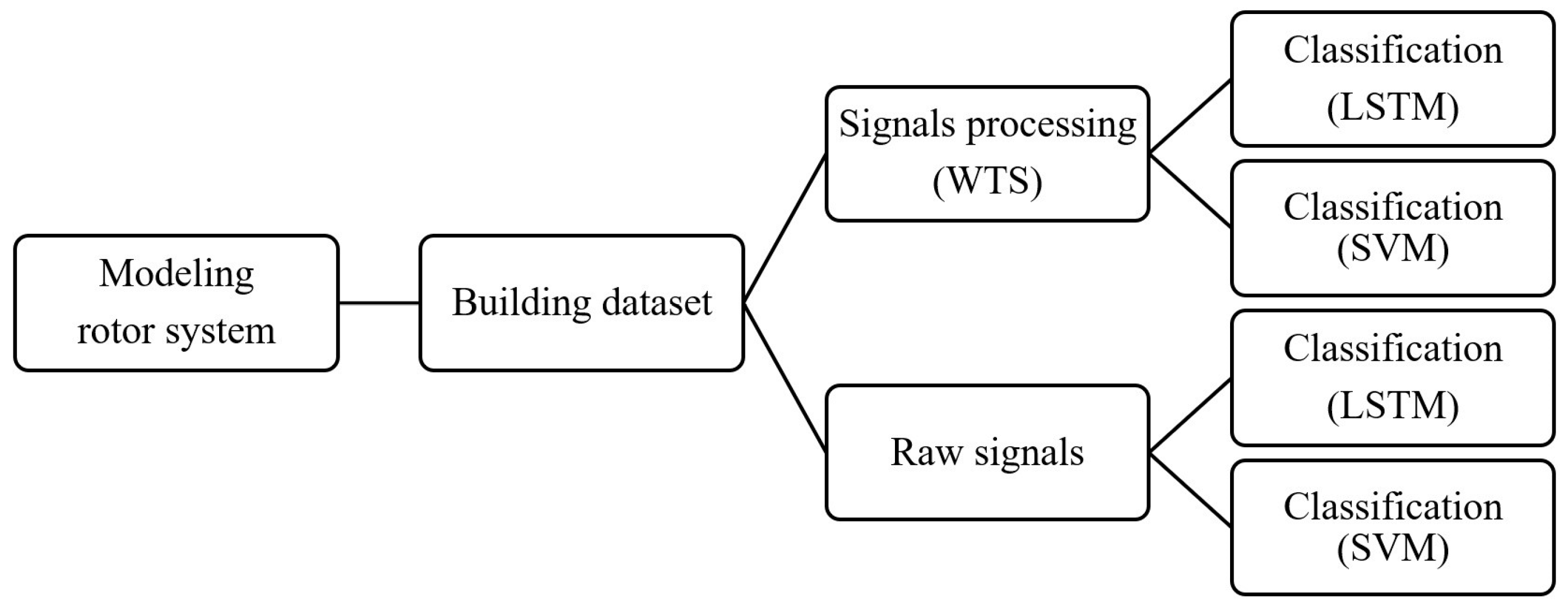
A data set is required to train the designed network and assess the effectiveness of the learning process when using classification algorithms. Unbalanced and bowed rotor systems should be modeled in ABAQUS/CAE first, and then the modeled systems should be run under various circumstances, such as changing the physical properties and operational conditions. The feature extraction phase is performed utilizing WTS to prepare inputs for the LSTM and SVM models. Additionally, the original time series data are applied in the classification using LSTM and the feature extraction material before applying the SVM to represent the effectiveness of the applied feature extraction method, i.e., WTS in the classification of unbalanced and bowed rotor systems.

The primary rationale behind the selection of LSTM and SVM for the classification phase stems from their distinct mechanisms in establishing relationships between independent and dependent variables. Specifically, LSTM has been engineered to discern temporal dependencies within sequential and time-series data, whereas SVM predominantly excels in identifying non-linear dependencies within the data set. Consequently, the observed outcomes ensuing from the application of these methodologies demonstrate that the employed feature extraction procedure, herein referred to as WTS (wavelet transform and statistical features), exhibits considerable efficacy in capturing dependencies in rotor systems signals, encompassing both temporal dynamics and non-linear characteristics. Figure 1 reveals the workflow of the present research.

2.1. Modeling in ABAQUS/CAE

ABAQUS allows modeling a fault in a system whether by variations in the geometry resulting from the damage such as a crack or by employing the expected force due to the defect such as a bearing defect in a rotary system by means of periodic loads. In this article, the first approach, i.e., change in the geometry of the system, is utilized to model faulty rotor systems.

As previously mentioned, an unbalancing occurs when the volume (geometry) and mass (mass) centers of a rotating object—in this case, a disk—are at different points. Figure 2a illustrates a schematic of an unbalanced rotor-disk-bearing system. The disk’s volume and mass centers are indicated in the figure by the letters C and M, respectively. On the other hand, a bowed shaft refers to a situation where the rod is not straight along its main axis. A schematic of this assumption is shown in Figure 2b (with exaggeration).

The modeled rotating system in ABAQUS in the current work consisted of a shaft, a central disk, and two couplings at the ends. The couplings are modeled as the kinematic type; as the boundary condition, the ends of the shaft are constrained in all directions except rotation around the fundamental axis of the shaft (x-axis). It should be mentioned that the shaft and disk are considered integrated parts. On the assumption of the bowed rotor, the shaft is drawn along a curved line, where the maximum curvature is in the center of the shaft. C3D8R solid elements (characterized by 8 nodes with 3 degrees of freedom per node) from the Abaqus Library were used to model both the shaft and the disk, using an average element size of 10 mm. For the bowed rotor, a total of 33,880 elements and 39,096 nodes were created.

To model unbalancing in the rotor system, a number of holes have been drilled in the disk. By changing their diameters as well as their distances from the disk’s center, the mass center of the disk changed (eccentricity has occurred). The FE model counts a total of 33,353 elements and 39,328 nodes which were created with the same solid elements as the bowed system. Graphs in Figure 3 are the meshed models of the unbalanced and bowed rotor systems, subsequently.

To determine the optimal mesh size, a mesh convergence test was conducted to analyze the L2 norm of transverse displacement, i.e., the y-axis in Figure 3 at the node of the left side journal bearing across different mesh sizes. The distinctions between the various mesh grid sizes were not stark. So, the most suitable sizes were chosen based on the aforementioned values.

The explicit dynamic procedure is performed to analyze the systems’ motion while the constant rotating velocity is modeled using a predefined field in the load module; vibration signals are captured in the transverse direction, e.g., y-axis.

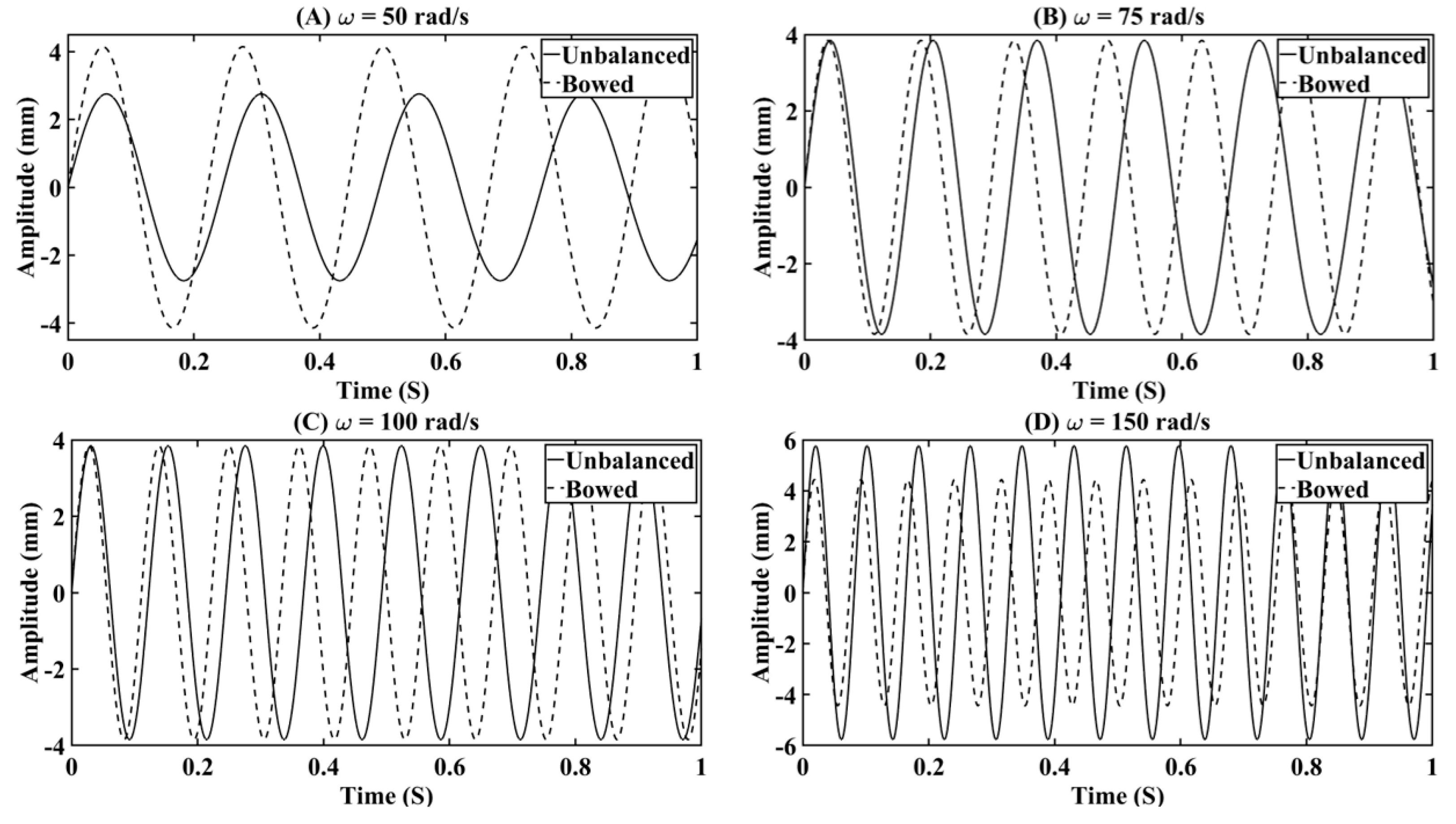
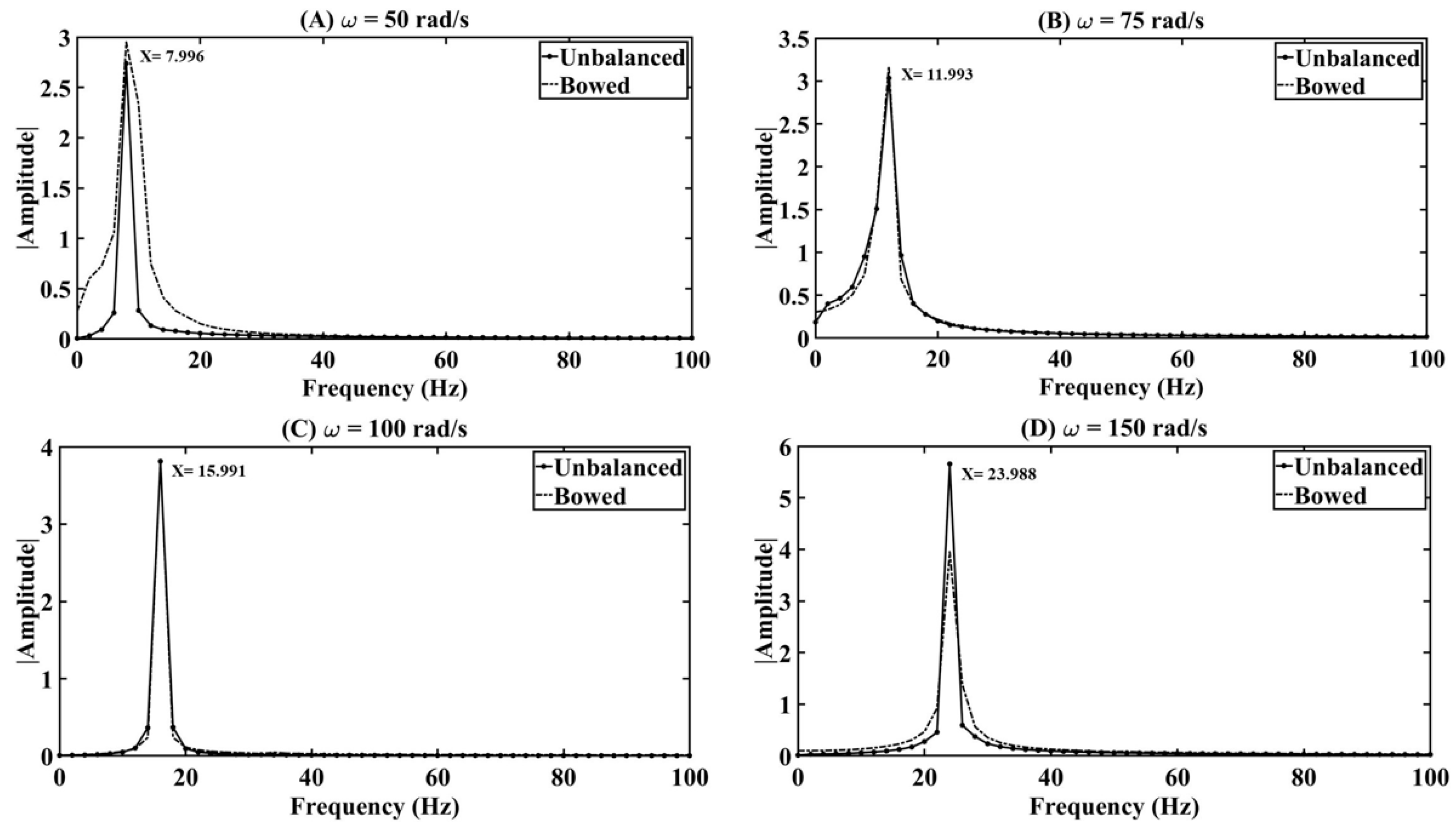
To compare vibration signals of the unbalanced and bowed rotor systems in the stationary performance, the time domain waves and frequency spectrums (single-side) for four operational speeds, i.e., 50, 75, 100, and 150 rad/s, are plotted in Figure 4 and Figure 5. Mechanical parameters of these four systems are selected the same as are listed in

Table 1. Parameters of the rotor system.

Parameter	Magnitude	Parameter	Magnitude
Shaft length	150 mm	Density	7.83 × 10−6 kg/mm3
Shaft diameter	100 mm	Young’s modulus	207,000 MPa
Disk diameter	300 mm	Poisson’s ratio	0.3
Disk width	100 mm	Structural damping	0.02

. To have a reasonable comparison between these two faults, amounts of the disk eccentricity and the initial bow are selected the same—5 mm. It is worthwhile to emphasize that to avoid resonance or semi-resonance behavior that can result in transient changes in the signal, these velocities are selected well below the first torsional natural frequency (subcritical speed range), e.g., 68.29 Hz (~429 rad/s).

It is crucial to mention that the values presented in Table 1 have been selected due to their close alignment with the dimensions of potential rotating systems that can be installed and studied in laboratory settings by future researchers. On the contrary, opting for smaller dimensions would restrict the achievable rotational speed, which hinders the analysis by diminishing the critical speed.

When the rotation pace was 75 and 100 rad/s, the vibration signals of the bowed and unbalanced systems were in the same range according to Figure 4. While in the slowest rotational speed, e.g., 50 rad/s, the vibration of the bowed system was more intensive than the unbalanced one; on the assumption of the fastest velocity (150 rad/s), on the contrary, the amplitude of the unbalanced system is much higher than the bowed rotor while the magnitude of the bowed systems remained approximately constant in all operational conditions. These behaviors find their roots in the unbalancing force’s nature, which is characterized by an increase in magnitude with the square of the rotational speed, as well as the shaft bow’s introduction of a roughly constant force [15,48]. Similar observations were noted in industrial scenarios, where the augmentation of rotational speed was found to be ineffectual in yielding a proportional increase in the resultant force of a shaft deflection [49].

In the frequency spectrums, the first frequency harmonic was observed at approximately the same rotational speeds that the systems operated; moreover, there are not any other higher harmonics neither in the unbalanced system nor in the bowed one. It should be noted that a second frequency component appeared when the Fourier transform’s sampling frequency was increased, but its amplitude and occurrence frequency were constant across all four operational speeds, indicating that it represented the system resonance frequency rather than the fault’s effect.

2.2. Building the Data Set

Since the main objective of the present study is to classify unbalanced and bowed rotary devices using artificial intelligence, a data set should be created by simulating the modeled systems in various contexts. Numerous classification algorithms, including both classic machine learning algorithms and deep neural networks, are data-hungry, which means as the number of sample tests falls, the network’s predictive accuracy decreases as well. To address the problem in the classification of faulted rotor systems, the combination of WTS with LSTM and SVM is proposed. As a result, the whole data set contains only 140 samples, where unbalanced and bowed systems, Class 1 and Class 2, respectively, have only 70 representatives.

2.3. Uncertainty

In rotor fault detection, uncertainty refers to the inherent variability and unpredictability in the physical and operational conditions of the rotary systems. This variability can cause variations in the signals generated by faulty systems, making it difficult to identify and classify the faults accurately. The uncertainty concept in rotor fault detection aims to account for these variations and ensure that the data set used for modeling and simulation represents the diverse conditions that the rotary systems may experience in real-world scenarios. By taking uncertainty into account, the goal is to develop more robust and reliable models for detecting and classifying rotor faults.

In the forming of the data set, the concept of uncertainty is employed. There are various sources of uncertainties in a system, such as model parameters, boundary conditions, external (operational) loads, faults, observations (measurements), and model uncertainty. All of them can be aleatory or epistemic in nature. Different techniques, such as the probabilistic distribution function (PDF), fuzzy (membership) function, and interval function, can be used to model uncertainty. Additionally, uncertainty can be quantified using either probabilistic or non-probabilistic methods. The first category includes methods such as Monte Carlo simulation, polynomial chaos expansion, random matrix theory, Bayesian inference, and Kriging surrogate, whereas the second category contains techniques, such as the fuzzy, evidence-based, imprecise, Taylor, and Chebyshev interval strategies [26]. The equation of motion of a rotary machine can be written as Equation (1):

MY″(t) + CY′(t) + KY(t) = F(t)

(1)

in which M, C, and K represent the mass, damping, and stiffness matrices, respectively. Furthermore, Y is the displacement vector, and F represents the force vector.

Since as mentioned earlier, the effects of faults are simulated by variations of the systems’ geometries in this work, uncertainties in the model parameters are considered to produce the sample tests. As a result, by changing the values of Young’s modulus and rotational speed, the modeling and simulation parameters of systems varied. To apply uncertainty in Young’s modulus, the probabilistic method with perturbation technique is used. If the initial value of Young’s modulus is E_j0, the jth uncertain parameter can be calculated using the following equation [50].

E_j = E_j0(1 + ε_j)

(2)

where ε_j is the jth uncertain parameter that should satisfy |ε_j| < 1. The data set is created by selecting five rotational speeds, 15, 50, 75, 100, and 150 rad/s; E_j is 207,000 MPa; uncertain parameters are then calculated for this parameter by applying Equation (2) until the 15th order. The perturbation term is selected between 0.001 and 0.09 with a constant increment. As a result, for each of the unbalanced and bowed systems, 70 samples are achieved.

Several key considerations support the selection of the five specified rotational speeds. Firstly, opting for values below the lower limit of 15 rad/s would result in a rotation that is excessively slow, making it difficult to clearly observe the noticeable effect of the shaft bow. Hence, values below this limit are deliberately avoided. Conversely, the upper limit of 150 rad/s has been carefully determined to effectively minimize the impact of imbalance, ensuring that it remains well below the first critical torsional speed and does not overshadow the bowing effects.

2.4. Signal Processing

Latent information can be extracted manually or automatically for classification purposes by converting original signals into numerical features, whether in the time, frequency, or time–frequency domain.

In some cases, extracted statistical features from raw data in the time domain, such as standard deviation and peak values, can result in significant accuracy in the classification algorithms although, on the assumption of signals in limited length and negligible differences of different classes, more sophisticated techniques such as wavelet transformation should be applied either in the classification or feature extraction process [51,52].

The Gabor (analytic Morlet) wavelet is utilized to construct a network for a WTS decomposition in MATLAB^®. WTS produces representations that are impervious to input signal translations without compromising class discriminability. The results of WTS typically give a hierarchical representation of the input signal, with each layer capturing different time–frequency features. The first layer records low-frequency information, and the succeeding layers collect information with an increasing frequency. These representations can be used as the input feature matrices of a classifier or regressor algorithm. In this technique, real-valued time series data should pass frequently through three steps consisting of convolution, non-linearity, and averaging using wavelet decomposition, modulus, and low-pass filter, respectively [52,53].

The number of filters per octave and the length of translation invariance are the only variables that must be determined for feature extraction and signal processing using WTS. Until the duration-based invariance scale (IS) is reached, the scattering framework is translation-invariant. The representation of the signal and the features that are derived from it both heavily depend on IS. To distinguish between patterns that are truly similar and those that are similar only by chance, a low degree of IS means that the transform can only detect patterns that are similar at a specific scale. Since the scaling filter is used to apply the invariance in the framework, its time support is not greater than that of the invariant. IS should be greater than the wavelet’s time support; IS has impacts on the center frequencies’ spacing in the filter banks. This parameter can be calculated by inverting the Fourier transform of the scaling function and centering it at 0 in time when the dynamical variations of the signals are known; otherwise, it can be discovered through trial and error [54,55].

In this study, the transverse vibration signal of each sample is recorded for 3 s with a sampling frequency of 4 kHz. To avoid transient behavior, the initial 1.55 s is disregarded, while the final 1.46 s is retained.

In accordance with the Nyquist–Shannon Sampling Theorem, the sampling frequency (in this case, 4 kHz) should be at least twice the maximum frequency component present in the signal (which is 23.98 Hz). Thus, the sampling frequency is chosen significantly higher than necessary to avoid missing any frequency components within the signals.

Given that the objective of the present investigation is to analyze the stationary signal of defective rotor systems, there are no specific restrictions on the time–wave range. Any section of the signals that represents stationary behavior can be appropriately incorporated into the methodology employed in this study.

The WTS technique is utilized with an IS of 0.5 and the original data’s sampling frequency to compute a coefficient matrix for each sample. The resulting matrix has a dimension of 199 × 12, representing 199 time–frequency representations generated by the WTS, each with 12 features. The feature matrix for the entire data set has a dimension of 140 × 199 × 12, where 140 is the total number of sample tests. These matrices will be used in the classification process, where they will be fed into both an LSTM network and SVM in subsequent stages.

2.5. Classification

Classification as a subfield of artificial intelligence can differentiate between two or more categories based on the extracted features. Thanks to the state of the art in this field, a machine learning (ML) network and its subfield, a deep learning (DL) network, can be used to perform intelligent tasks, such as classification, regression, and anomaly detection. The number of node layers—or depth—of ML and DL networks is the key distinction: In a deep network, the number of hidden layers ought to be two or more [56].

Utilizing recurrent neural networks (RNNs) such as LSTM and convolutional neural networks (CNNs), deep learning can be performed on sequence data and time series data and visual objects (such as images). With memory cells and recurrent connections, LSTM is a feedforward neural network (nodes do not form loops). As an optimized neural network algorithm, LSTM manages long-term dependencies (with the LSTM layer), explores gradients, and handles vanishing problems.

There are three various gates in an LSTM, i.e., input, output, and forget that have the responsibility of conducting information throughout the network in such a way that the network decides which information is kept and which to be discarded through the gates. This property gives LSTMs further capability for remembering information rather than the other types of RNNs.

An LSTM network normally consists of various layers, which include an input layer, one or more LSTM layers, an output layer, and optionally, fully connected layers. The entry point for data is the input layer while the LSTM layers are fundamental layers containing the LSTM cells, which handle the input data and preserve the network’s internal state. The output layer receives the output from the LSTM cells and generates a prediction of output. Fully connected layers can be used for classification or regression tasks and map the output of the LSTM layers to a specific output size or range. To enhance the network’s ability to learn complex patterns, an activation layer can also be added to introduce non-linearity. It should be noted, however, that the number of layers, LSTM cells, and fully connected layers may need to be adjusted based on the specific task and data set to achieve optimal performance [57,58].

One of the most popular supervised machine learning models, support vector machine (SVM) as non-parametric model has demonstrated its effectiveness in both classification (SVC) and regression (SVR) tasks. Along with its solidity against model errors, the technique’s fundamental advantage is its ability to handle a small number of features with reasonable accuracy as well as explore non-linear dependencies in the data [59].

SVM can be performed in a data set where features of two or more classes are distinguishable in a linear also non-linear approach using the optimal hyperplane (the separation plane). A kernel made up of a set of mathematical functions can be employed to modify the input data when the condition indicators of classes are non-linear. There are several types of kernels, such as Dirichlet, Sigmoid, radial basis function, polynomial, and Gaussian. The polynomial kernel itself can be divided into cubic, quadratic, etc., based on its order [60,61].

This work utilizes LSTM as a supervised deep network and SVM as a supervised machine learning algorithm to categorize faulted systems into Class 1 and Class 2 (with indices 0 and 1 as the labels in the data set for the unbalanced and bowed rotors, respectively).

These two classification models were chosen because of how well they each do at determining the connection between the input data and the intended response. While SVM can identify non-linear reliance, LSTM was developed to reveal short- and long-term subordinations. However, it should be noted that the entire procedure was examined by fewer number of observations, and the employed numbers are the lower required limit for the current use. As a result, performing the models can reveal WTS’s competence in extracting meaningful condition indicators regardless of what classification model is to be applied and/or how many training materials are achievable.

The extracted coefficients of WTS should be inserted into the LSTM network in the first mechanism, to memorize the time dependencies. Hyperparameters of the employed LSTM network are listed in

Table 2. The LSTM network’s hyperparameters.

Option	Value	Option	Value
Mini batch size	12	Learning rate	1 × 10−4
Maximum epoch	500	Validation frequency	30
Number of hidden layers	512	Shuffle	Every epoch

; stochastic gradient descent with momentum (SGDM) optimizer is applied as the solver. The choice for the state activation function was the hyperbolic tangent function (tanh).

In the second part, the explored WTS feature should be added to the SVM model by using parameters outlined in

Table 3. The SVM network’s hyperparameters.

Option	Value	Option	Value
Kernel type	Quadratic	Box constraint level	1
Kernel scale	Auto	Standardize data	True
Multiclass method	One-vs-One	Cross-validation folds	5

. It is worthwhile to mention that the cross-validation technique is used for the validation (protecting from overfitting). Similar to the WTS procedure, both classification methods are applied in MATLAB^®.

It should be mentioned that these hyperparameters have been tuned by comparing the training and testing accuracies in various scenarios utilizing a grid search optimization procedure with the number of grid divisions equal to 20. Worthwhile to note that these hyperparameters were optimized based on the performance of the network trained by extracted health indicators utilizing WTS.

2.6. Evaluating Metrics

Valid metrics assessment should be implemented for managing the performance of artificial intelligence models, whether controlled manually by a user or automatically (in problems governed by optimization algorithms). Accuracy, precision, recall, F1-Score, and root mean squared error can be mentioned as well-known examples.

Before delving into the analysis of these metrics and presenting the corresponding equations, it is crucial to establish a clear understanding of certain fundamental concepts. Let us consider a scenario where the objective entails the classification of shapes into two distinct categories: “circle” and “cube”.

The term “true positive” (TP) refers to the count of instances that belong to the positive class (i.e., circles) and have been accurately predicted as such. Conversely, the designation “true negative” (TN) encompasses the instances belonging to the negative class (i.e., cubes) that have been correctly identified as such in the predictions.

Conversely, “false positive” (FP) signifies the instances that pertain to the positive class (circles) but have been erroneously predicted as belonging to the negative class (cubes). On the other hand, “false negative” (FN) denotes the instances that belong to the negative class (cubes) but have been incorrectly identified as members of the positive class (circles).

Accuracy can be defined as the ratio of the correctly classified samples to the overall number of instances and normally is stated as a percentage; precision, on the other hand, measures the percentage of correctly predicted positive instances among all positive instances that were predicted. It focuses on the reliability of optimistic forecasts and evaluates how well the model does at reducing false positives. The proportion of correctly predicted positive instances among all actual positive instances is measured by recall (also known as sensitivity or true positive rate). It is helpful in applications where false negatives should be minimized because it concentrates on correctly identifying all positive instances.

The harmonic means of recall and precision is known as the F1-Score. It offers a fair evaluation of both recall and precision, giving each metric the same weight [62].

Based on the values of TP, TN, FP, and FN, the following formulas provide a mathematical definition for the stated metrics.

Accuracy = (TP + TN)/(TP + TN + FP + FN)

(3)

Precision = TP/(TP + FP)

(4)

Recall = TP/(TP + FN)

(5)

F1-Score = 2 × (Precision × Recall)/(Precision + Recall)

(6)

The mentioned metrics will be utilized further in the Results section to represent the designed classification models along with the feature extraction procedure.

3. Results and Discussion

The training material is drawn randomly from 80% of the whole data set; the testing material is taken from the remaining 20%. In both the training and testing phases, each class has an equal share, e.g., 56 and 14, respectively. As a means of comparing the two proposed classification approaches fairly, the training and testing samples from the first algorithm, that is, the LSTM, are saved to be applied in the second method as well.

Initially, the extracted features from the WTS were fed into the designed classification models. In Figure 6, the training progression is plotted along with the accuracy and loss for each epoch in the LSTM network. The training process was run on a single GPU (NVIDIA Quadro P2000) of a workstation and took 75 s. From Figure 6, it can be understood that the training accuracy increased gradually parallel with a sensible reduction in loss after each epoch.

The confusion matrices in the training and testing steps are also represented by the graphs in Figure 7. Only 1 sample out of the 112 that were assigned to the training process is incorrectly classified in the validation, despite the testing accuracy being 100%.

Figure 8 presents the confusion matrices of the training and testing phases when the SVM model is applied as the classifier for the explored features by the WTS. The training accuracy in the method was 100%, whereas, in the testing phase, 1 sample among the 28 samples, e.g., 3.6%, is classified mistakenly. Even though there has been a drop in performance between the training and testing phases, a 3.6% drop in performance does not necessarily mean that the network is overfitted. When a network becomes excessively customized to the training data and then performs horribly on unobserved test data, this is known as overfitting. The problem’s inherent complexity and variations in the test data, such as outliers, can both result in a 3.6% reduction in performance.

The whole procedure of executing WTS and SVM on the same workstation in a single GPU took only 42 s.

Now that the previous two classification algorithms have been trained and tested using features extracted by WTS, the same procedures should be tested with raw signals. There are two possible methods for using LSTM for time series signals: The first is to feed the signals directly into the network, while the second is to apply a feature extraction step before the LSTM network; in this work, the first approach is followed.

The same parameters listed in Table 2 were used to insert the time series data into the LSTM network directly, and both the training and testing phases produced an accuracy of 50% (the confusion matrices are not plotted); indeed, the network assigned Class 1 to every system that had a fault.

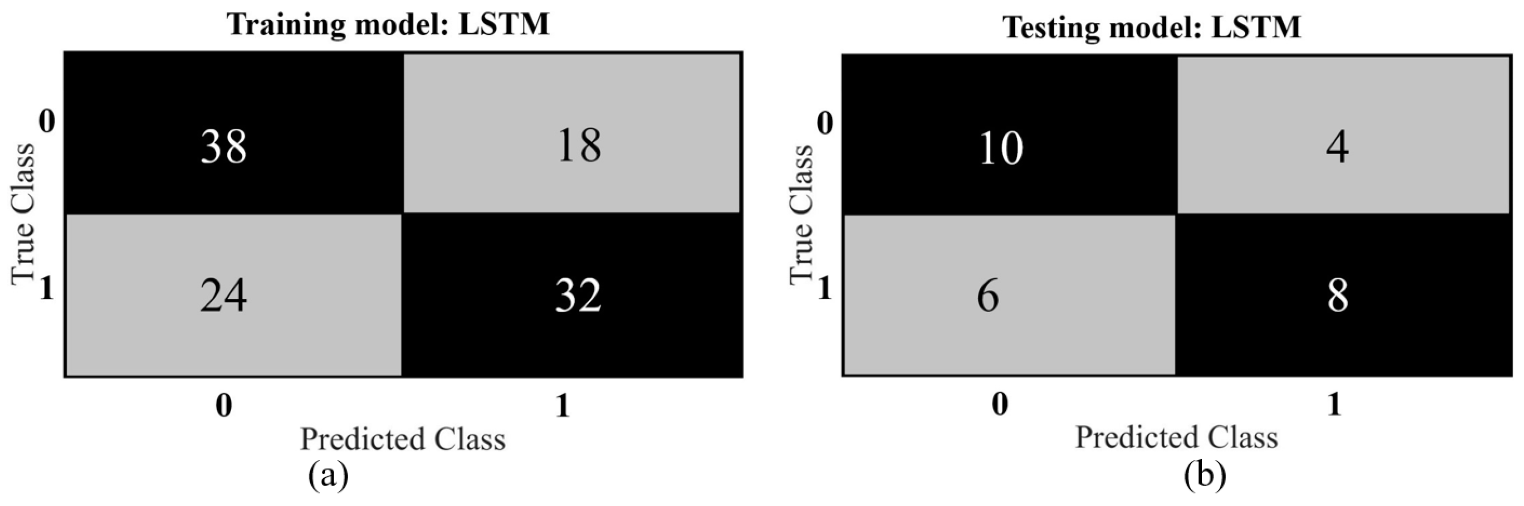
Performing hyperparameters tunning via a grid division tantamount to 20, the accuracy in both steps—training and testing—improved by 62.5% and 64.3%, respectively. On this condition, the optimized learning rate, hidden layers, mini-batch size, and maximum epoch were found to be 0.2, 4000, 9, and 1000, respectively. However, the outcomes are still far from the previously attained feature extraction and trained LSTM model.

Figure 9 represents the training and testing stages’ performance of the adjusted LSTM network in the form of confusion matrices.

The effectiveness of LSTM models in analyzing raw signals was investigated in previous sections. The results, however, demonstrate that the raw signals are not highly instructive. As a result, in this section, a different feature extraction strategy is aimed to be examined. The objective is to assess this new scenario’s effectiveness before putting the created SVM model to use for classification. To this end, 10 features from each sample test are extracted, including kurtosis, skewness, root mean square, signal-to-noise ratio, total harmonic distortion, variance, standard deviation, spurious free dynamic range, band power, and Shannon entropy. It should be noted that the training and testing data sets are selected the same as the previous sections.

The training and testing phases’ accuracies—83.9% and 89.3%, respectively—increased significantly when the SVM was applied to the extracted features from the time series data in comparison to the earlier technique, which involved using LSTM on the raw data. It is important to acknowledge that the hyperparameters are chosen similarly to the previous SVM network. Confusion matrices of training and testing steps on this condition are plotted in Figure 10.

To have a clearer assessment, other defined metrics, i.e., recall, precision, and F1 score, in both input scenarios, i.e., raw signal and engineered features, are calculated from formulas 4 to 6 for the training and testing steps and presented for the LSTM and SVM models in

Table 4. Metrics for LSTM classification model.

Metric	Phase
	Training		Testing
	Input		Input
	WTS	Raw Signal	WTS	Raw Signal
TP	55	38	14	10
TN	56	32	14	8
FP	0	24	0	6
FN	1	18	0	4
Accuracy (%)	99.11	62.5	100	64.29
Precision (%)	100	61.29	100	62.5
Recall (%)	98.21	67.86	100	71.43
F1-Score (%)	99.09	64.47	100	66.67

and

Table 5. Metrics for SVM classification model.

Metric	Phase
	Training		Testing
	Input		Input
	WTS	Second Scenario	WTS	Second Scenario
TP	56	46	14	13
TN	56	48	13	12
FP	0	8	1	2
FN	0	10	0	1
Accuracy (%)	100	83.93	96.43	82.29
Precision (%)	100	85.19	93.33	86.67
Recall (%)	100	82.14	100	92.86
F1-Score (%)	100	83.62	96.55	89.66

, respectively.

Comparing the statistics of Table 4 and Table 5, it can be understood that a signal processing (feature extraction) step to how extend can increase the performance of the classification model. Indeed, the applied WTS increases the dimensionality of raw signals to provide more ingredients for training the model. Additionally, research shows that using slightly more straightforward feature engineering methods and increasing the number of observations under the SVM assumption probably can also lead to acceptable results.

4. Conclusions

This article examined the performance of combinations of WTS with LSTM and SVM employed in the classification of unbalanced and bowed rotor systems. Additionally, changing the mass center and central axis of the shaft, respectively, allowed for the initial modeling of unbalanced and bowed coupled-rotor-disk systems using the finite element method in ABAQUS/CAE. Both methodologies present a novelty for structural health monitoring (SHM).

The results of the modeled systems were compared in four simulation statuses together, i.e., the same physical properties operated in various rotational paces as well as the tantamount magnitude of unbalancing and initial bow. By applying concepts of uncertainties in model parameters, 70 different physical and operational circumstances were simulated for each of the rotating systems. Wavelet time scattering was used to perform the signal processing stage by extracting the scattered wavelet coefficients. Using a long short-term memory network as a deep learning algorithm for time series data, a hit rate of 100% was obtained running a maximum of 500 epochs in the testing phase. In the training step, the achieved accuracy was noticeable too, e.g., 99.1%. Training the LSTM network with the raw time series data, on the contrary, showed a faint performance—50% in both the training and testing stages although by adjusting the hyperparameters of the network, the accuracies in the training and testing phases developed to 62.5% and 64.3%, respectively.

While considering SVM along with WTS, the training accuracy in the method was 100%, whereas, in the testing phase, 1 sample among the 28 samples (3.6%) was classified wrongly. Considering SVM without WTS, the hit rate was 83.9% and 89.3%, respectively. The results of feature extraction in the time domain and the application of SVM also demonstrated the possibility of classifying such flawed systems in the case of setting hyperparameters and/or extracting more robust features.

Ultimately, although the limited number of samples in a data set (140 overall), the methods employed in this paper showed high accuracy in classifying unbalanced and bowed rotor systems; therefore, rendering this approach a promising and useful contribution to the SHM area. Future work will focus on modeling rotor systems suffering from other prevalent defects, such as cracks, bearing faults, and misalignment, and applying the proposed benchmark in the case of multi-damaged systems. Furthermore, the applicability of the proposed fault classification algorithm can be validated utilizing experimental data whether from test rigs or real operating machines installed in the industry.