
Deep Learning Architectures for Diagnosis of Diabetic Retinopathy

 , ,
, ,
Abstract
:1. Introduction
2. Materials and Methods
2.1. DRIVE Dataset
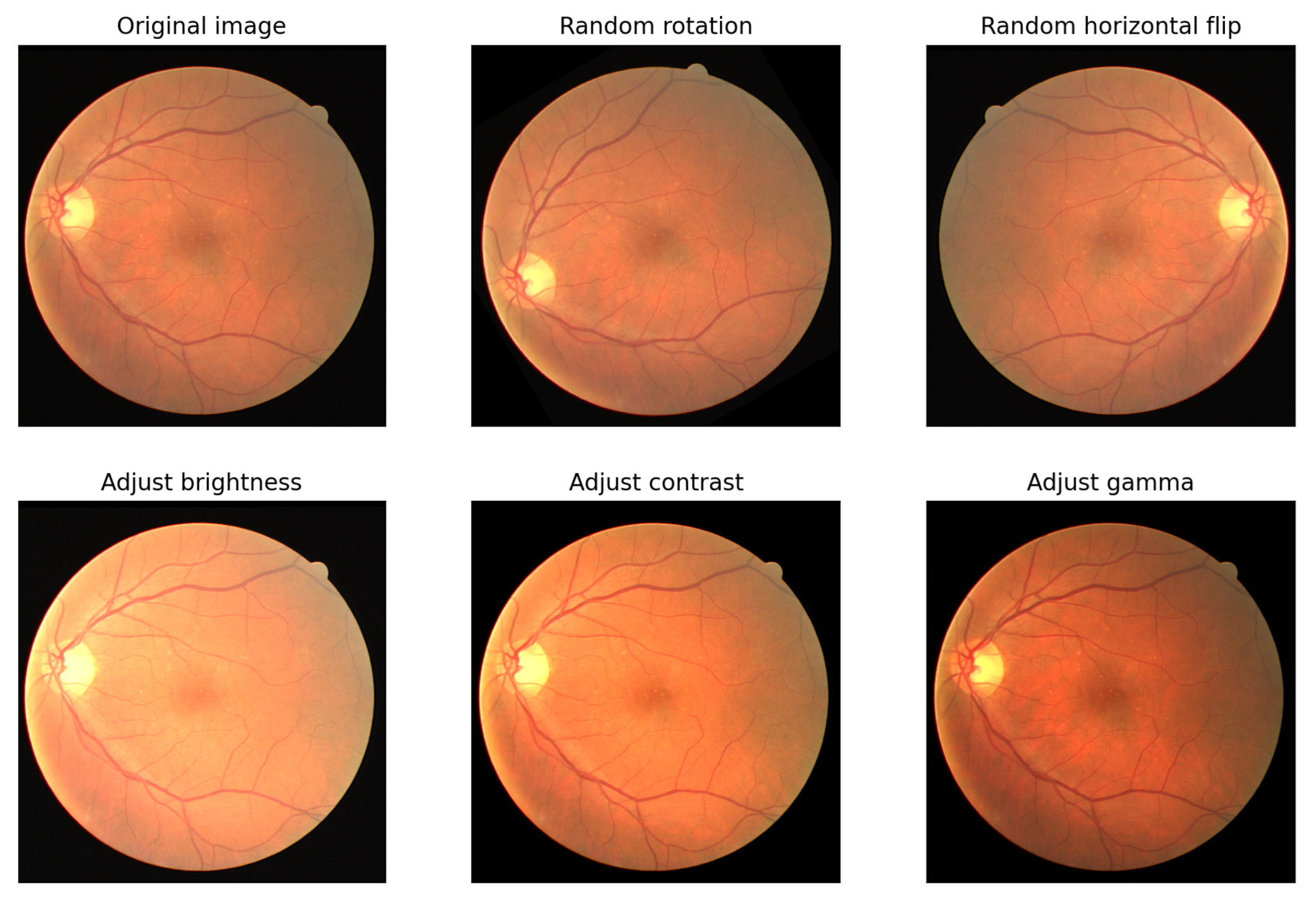
2.1.1. Data Augmentation
- Random rotation: Always applied, with lower and upper bounds for the rotation angle given by parameter , i.e., rad.
- Random horizontal flip: With probability .
- Brightness adjustment: Being applied 10% of the time with a random factor between an upper and lower bound , where gives a complete black image, leaves the original image unchanged and increases the brightness by that factor.
- Contrast adjustment: Furthermore, being applied with a probability of 10%, based on a factor between an upper and lower bound , where gives a solid gray image, leaves the original image unchanged and increases the contrast by that factor.
- Gamma correction: Known as Power Law Transform, applied again with a probability of 10% with a fixed factor of 1 and a random factor, again between some upper and lower bounds around 1. Values smaller than 1 make the dark regions lighter while values larger than 1 make the shadows darker.
- Random affine: Transformation of the image with probability , keeping the center invariant. It combines a translation in both x and y directions, i.e., and , plus a random zoom of the image up to a maximum and, also, an x-shearing parameterized between two values .
- Random gaussian noise: With a fixed zero-mean () and a variable standard deviation .
2.2. Data Augmentation Hyperparameter Tuning
2.3. Evaluation Metric
2.4. Loss Function
2.5. Models
2.5.1. CNN’s Models: U-Net
2.5.2. ViT Models: UNETR and Swin-UNET
2.5.3. ConvMixer
2.6. Training Considerations
3. Results
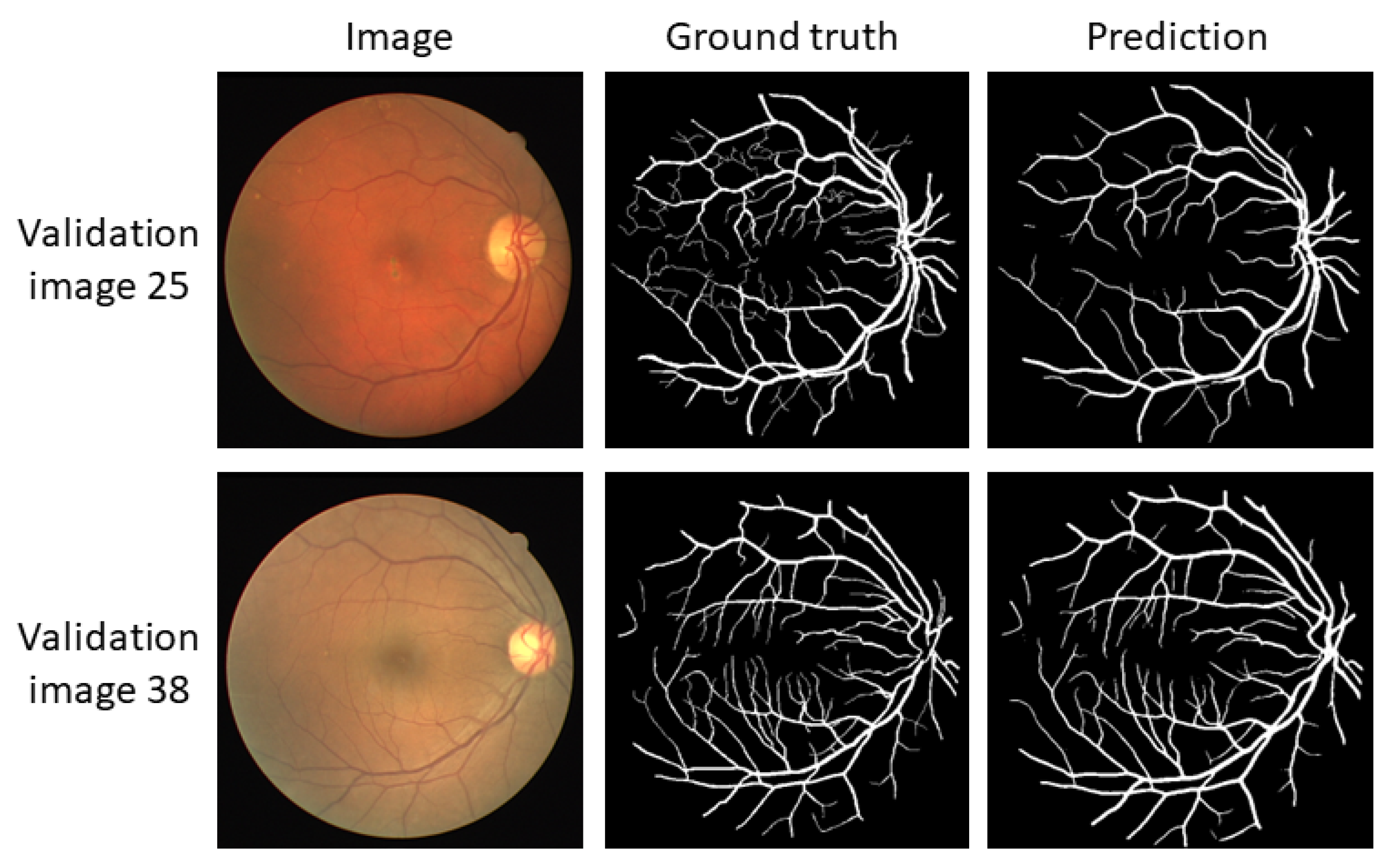
3.1. U-Net
3.2. ViT’s: UNETR y Swin-UNET
3.3. Convmixer
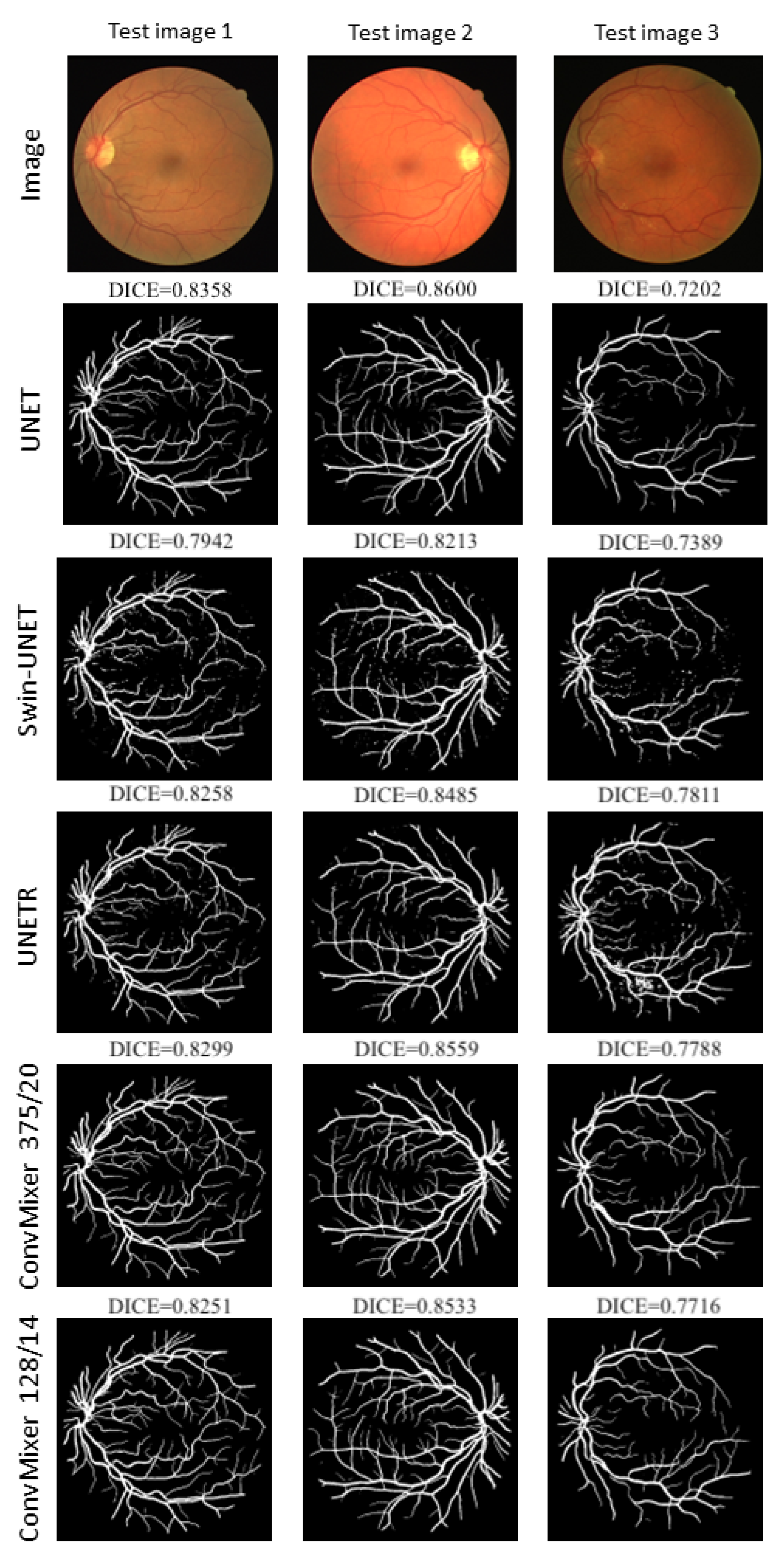
3.4. Summary
4. Discussion
Author Contributions
Funding
Institutional Review Board Statement
Informed Consent Statement
Data Availability Statement
Acknowledgments
Conflicts of Interest
Abbreviations
| CNNs | Convolutional Neural Networks |
| ViT | Vision Transformer |
| DRIVE dataset | Digital Retinal Images for Vessel Extraction dataset |
| STARE dataset | STructured Analysis of the Retina dataset |
| CHASE dataset | Child Heart and Health Study in England dataset |
| TP | True Positive |
| FP | False Positive |
| FN | False Negative |
| IoU | Intersection over Union |
| BCE | Binary Cross-Entropy |
References
- McGlinchy, J.; Johnson, B.; Muller, B.; Joseph, M.; Diaz, J. Application of UNet Fully Convolutional Neural Network to Impervious Surface Segmentation in Urban Environment from High Resolution Satellite Imagery. In Proceedings of the IGARSS 2019—2019 IEEE International Geoscience and Remote Sensing Symposium, Yokohama, Japan, 28 July–2 August 2019; pp. 3915–3918. [Google Scholar] [CrossRef]
- Pesaresi, M.; Benediktsson, J.A. A new approach for the morphological segmentation of high-resolution satellite imagery. IEEE Trans. Geosci. Remote. Sens. 2001, 39, 309–320. [Google Scholar] [CrossRef] [Green Version]
- Nemni, E.; Bullock, J.; Belabbes, S.; Bromley, L. Fully convolutional neural network for rapid flood segmentation in synthetic aperture radar imagery. Remote. Sens. 2020, 12, 2532. [Google Scholar] [CrossRef]
- Xie, B.; Li, S.; Li, M.; Liu, C.H.; Huang, G.; Wang, G. SePiCo: Semantic-Guided Pixel Contrast for Domain Adaptive Semantic Segmentation. IEEE Trans. Pattern Anal. Mach. Intell. 2022. [Google Scholar] [CrossRef]
- Antonelli, M.; Reinke, A.; Bakas, S.; Farahani, K.; AnnetteKopp-Schneider, A.; Landman, B.A.; Litjens, G.; Menze, B.; Ronneberger, O.; Summers, R.M.; et al. The Medical Segmentation Decathlon. Nat. Commun. 2021, 13, 4128. [Google Scholar] [CrossRef] [PubMed]
- Tsoukas, V.; Boumpa, E.; Giannakas, G.; Kakarountas, A. A Review of Machine Learning and TinyML in Healthcare. In Proceedings of the 25th Pan-Hellenic Conference on Informatics, New York, NY, USA, 26–28 November 2021; pp. 69–73. [Google Scholar] [CrossRef]
- Fong, D.S.; Aiello, L.; Gardner, T.W.; King, G.L.; Blankenship, G.; Cavallerano, J.D.; Ferris, F.L., III; Klein, R.; for the American Diabetes Association. Retinopathy in Diabetes. Diabetes Care 2004, 27, s84–s87. [Google Scholar] [CrossRef] [PubMed] [Green Version]
- Kaur, J.; Agrawal, S.; Renu, V. A Comparative Analysis of Thresholding and Edge Detection Segmentation Techniques. Int. J. Comput. Appl. 2012, 39, 29–34. [Google Scholar] [CrossRef]
- Zhu, S.; Xia, X.; Zhang, Q.; Belloulata, K. An image segmentation algorithm in image processing based on threshold segmentation. In Proceedings of the 2007 Third International IEEE Conference on Signal-Image Technologies and Internet-Based System, Shanghai, China, 16–18 December 2007; pp. 673–678. [Google Scholar]
- Gupta, A.; Issac, A.; Dutta, M.K.; Hsu, H.H. Adaptive Thresholding for Skin Lesion Segmentation Using Statistical Parameters. In Proceedings of the 2017 31st International Conference on Advanced Information Networking and Applications Workshops (WAINA), Taipei, Taiwan, 27–29 March 2017; pp. 616–620. [Google Scholar]
- Al-Amri, S.S.; Kalyankar, N.; Khamitkar, S. Image segmentation by using edge detection. Int. J. Comput. Sci. Eng. 2010, 2, 804–807. [Google Scholar]
- Canny, J. A Computational Approach to Edge Detection. IEEE Trans. Pattern Anal. Mach. Intell. 1986, PAMI-8, 679–698. [Google Scholar] [CrossRef]
- Yu, W.; Fritts, J.; Sun, F. A hierarchical image segmentation algorithm. In Proceedings of the IEEE International Conference on Multimedia and Expo, Lausanne, Switzerland, 26–29 August 2002; Volume 2, pp. 221–224. [Google Scholar] [CrossRef]
- Dhanachandra, N.; Manglem, K.; Chanu, Y.J. Image Segmentation Using K -means Clustering Algorithm and Subtractive Clustering Algorithm. Procedia Comput. Sci. 2015, 54, 764–771. [Google Scholar] [CrossRef] [Green Version]
- Mahony, N.O.; Campbell, S.; Carvalho, A.; Harapanahalli, S.; Velasco-Hernández, G.A.; Krpalkova, L.; Riordan, D.; Walsh, J. Deep Learning vs. Traditional Computer Vision. Adv. Comput. Vis. 2019, 943, 128–144. [Google Scholar] [CrossRef] [Green Version]
- Ronneberger, O.; Fischer, P.; Brox, T. U-Net: Convolutional Networks for Biomedical Image Segmentation. In Proceedings of the Medical Image Computing and Computer-Assisted Intervention—MICCAI 2015; Navab, N., Hornegger, J., Wells, W.M., Frangi, A.F., Eds.; Springer International Publishing: Cham, Switzerland, 2015; pp. 234–241. [Google Scholar]
- Vaswani, A.; Shazeer, N.; Parmar, N.; Uszkoreit, J.; Jones, L.; Gomez, A.N.; Kaiser, L.; Polosukhin, I. Attention Is All You Need. Adv. Neural Inf. Process. Syst. 2017, 30, 1–11. [Google Scholar]
- Dosovitskiy, A.; Beyer, L.; Kolesnikov, A.; Weissenborn, D.; Zhai, X.; Unterthiner, T.; Dehghani, M.; Minderer, M.; Heigold, G.; Gelly, S.; et al. An Image is Worth 16 × 16 Words: Transformers for Image Recognition at Scale. arXiv 2020, arXiv:2010.11929. [Google Scholar]
- Liu, Z.; Lin, Y.; Cao, Y.; Hu, H.; Wei, Y.; Zhang, Z.; Lin, S.; Guo, B. Swin Transformer: Hierarchical Vision Transformer using Shifted Windows. arXiv 2021, arXiv:2103.14030. [Google Scholar]
- Trockman, A.; Kolter, J.Z. Patches Are All You Need? arXiv 2022, arXiv:2201.09792. [Google Scholar]
- Tolstikhin, I.O.; Houlsby, N.; Kolesnikov, A.; Beyer, L.; Zhai, X.; Unterthiner, T.; Yung, J.; Steiner, A.; Keysers, D.; Uszkoreit, J.; et al. Mlp-mixer: An all-mlp architecture for vision. Adv. Neural Inf. Process. Syst. 2021, 34, 24261–24272. [Google Scholar]
- Staal, J.; Abramoff, M.; Niemeijer, M.; Viergever, M.; van Ginneken, B. Ridge-based vessel segmentation in color images of the retina. IEEE Trans. Med. Imaging 2004, 23, 501–509. [Google Scholar] [CrossRef] [PubMed]
- Hoover, A.D.; Kouznetsova, V.; Goldbaum, M. Locating Blood Vessels in Retinal Images by Piece-wise Threhsold Probing of a Matched Filter Response. IEEE Trans. Med. Imaging 2000, 19, 203–210. [Google Scholar] [CrossRef] [Green Version]
- Fraz, M.M.; Remagnino, P.; Hoppe, A.; Uyyanonvara, B.; Rudnicka, A.R.; Owen, C.G.; Barman, S.A. An Ensemble Classification-Based Approach Applied to Retinal Blood Vessel Segmentation. IEEE Trans. Biomed. Eng. 2012, 59, 2538–2548. [Google Scholar] [CrossRef]
- Toan, N.Q. Aiding Oral Squamous Cell Carcinoma diagnosis using Deep learning ConvMixer network. medRxiv 2022. [Google Scholar] [CrossRef]
- Tang, F.; Wang, L.; Ning, C.; Xian, M.; Ding, J. CMU-Net: A Strong ConvMixer-based Medical Ultrasound Image Segmentation Network. arXiv 2022, arXiv:2210.13012. [Google Scholar]
- Center, R.U.M. DRIVE: Digital Retinal Images for Vessel Extraction—Grand Challenge. Available online: https://drive.grand-challenge.org/ (accessed on 28 March 2023).
- Boudegga, H.; Elloumi, Y.; Akil, M.; Hedi Bedoui, M.; Kachouri, R.; Abdallah, A.B. Fast and efficient retinal blood vessel segmentation method based on deep learning network. Comput. Med. Imaging Graph. 2021, 90, 101902. [Google Scholar] [CrossRef] [PubMed]
- Biewald, L. Experiment Tracking with Weights and Biases. 2020. Available online: www.wandb.com (accessed on 28 March 2023).
- Hatamizadeh, A.; Tang, Y.; Nath, V.; Yang, D.; Myronenko, A.; Landman, B.; Roth, H.; Xu, D. UNETR: Transformers for 3D Medical Image Segmentation. arXiv 2021, arXiv:2103.10504. [Google Scholar]
- Cao, H.; Wang, Y.; Chen, J.; Jiang, D.; Zhang, X.; Tian, Q.; Wang, M. Swin-Unet: Unet-like Pure Transformer for Medical Image Segmentation. arXiv 2021, arXiv:2105.05537. [Google Scholar]
- Li, L.; Verma, M.; Nakashima, Y.; Nagahara, H.; Kawasaki, R. IterNet: Retinal Image Segmentation Utilizing Structural Redundancy in Vessel Networks. In Proceedings of the IEEE Winter Conference on Applications of Computer Vision (WACV), Snowmass Village, CO, USA, 1–5 March 2020. [Google Scholar]
- Azad, R.; Asadi-Aghbolaghi, M.; Fathy, M.; Escalera, S. Bi-directional ConvLSTM U-Net with densley connected convolutions. In Proceedings of the IEEE/CVF International Conference on Computer Vision Workshops, Seoul, Republic of Korea, 27–28 October 2019. [Google Scholar]
- Zhuang, J. LadderNet: Multi-path networks based on U-Net for medical image segmentation. arXiv 2018, arXiv:1810.07810. [Google Scholar]
- Kamran, S.A.; Hossain, K.F.; Tavakkoli, A.; Zuckerbrod, S.L.; Sanders, K.M.; Baker, S.A. RV-GAN: Segmenting retinal vascular structure in fundus photographs using a novel multi-scale generative adversarial network. In Proceedings of the International Conference on Medical Image Computing and Computer-Assisted Intervention, Strasbourg, France, 27 September–1 October 2021; pp. 34–44. [Google Scholar]
- Ban, Y.; Wang, Y.; Liu, S.; Yang, B.; Liu, M.; Yin, L.; Zheng, W. 2D/3D Multimode Medical Image Alignment Based on Spatial Histograms. Appl. Sci. 2022, 12, 8261. [Google Scholar] [CrossRef]
- Qin, X.; Ban, Y.; Wu, P.; Yang, B.; Liu, S.; Yin, L.; Liu, M.; Zheng, W. Improved Image Fusion Method Based on Sparse Decomposition. Electronics 2022, 11, 2321. [Google Scholar] [CrossRef]
- Liu, H.; Liu, M.; Li, D.; Zheng, W.; Yin, L.; Wang, R. Recent Advances in Pulse-Coupled Neural Networks with Applications in Image Processing. Electronics 2022, 11, 3264. [Google Scholar] [CrossRef]


| Dataset | Training (Labeled) Images | Testing (Unlabeled) Images | Resolution |
|---|---|---|---|
| DRIVE | 20 | 20 |
| Model | |||||||||||
|---|---|---|---|---|---|---|---|---|---|---|---|
| U-Net | [−180, 180] | 0.4 | [0.8, 1.2] | [0.8, 1.2] | [0.9, 1.1] | 0.3 | [0, 0] | [−0.1, 0.1] | ×1.20 | [0, 0] | 0.1 |
| UNETR | [−15, 15] | 0.3 | [0.5, 1.5] | [0.6, 1.5] | [0.7, 1.3] | 0.2 | [−0.1, 0.1] | [−0.1, 0.1] | ×1.25 | [0, 0] | 0.08 |
| Swin-Unet | [−45, 45] | 0.5 | [0.6, 1.4] | [0.6, 1.4] | [0.7, 1.3] | 0.2 | [−0.05, 0.05] | [−0.05, 0.05] | ×1.20 | [0, 0] | 0.05 |
| ConvMixer | [−45, 45] | 0.3 | [0.3, 1.7] | [0.3, 1.8] | [0.5, 1.5] | 0.15 | [−0.2, 0.2] | [−0.2, 0.2] | ×1.25 | [−0.1, 0.1] | 0.1 |
| ConvMixer-Light | [−45, 45] | 0.3 | [0.6, 1.6] | [0.6, 1.6] | [0.7, 1.5] | 0.15 | [−0.1, 0.1] | [−0.1, 0.1] | ×1.25 | [0, 0] | 0.05 |
| Network | Type | Params. | Val DICE | Test DICE | Process. Time (s) |
|---|---|---|---|---|---|
| U-Net | CNN | 31M | 81 | 82 | 8.1 |
| UNETR | ViT | 104M | 80 | 80 | 16.0 |
| Swin-Unet | ViT | 27M | 76 | 77 | 6.5 |
| ConvMixer | CNN | 2.97M | 82 | 83 | 11.0 |
| ConvMixer-Light | CNN | 0.27M | 82 | 82 | 4.2 |
| IterNet [32] | CNN | 13.6M | - | 82.18 | - |
| BCDU-Net [33] | CNN-RNN | 20.7M | - | 82.24 | - |
| LadderNet [34] | CNN | 1.5M | - | 82.02 | - |
| RV-GAN [35] | GAN | >14M | - | 86.90 | - |
Disclaimer/Publisher’s Note: The statements, opinions and data contained in all publications are solely those of the individual author(s) and contributor(s) and not of MDPI and/or the editor(s). MDPI and/or the editor(s) disclaim responsibility for any injury to people or property resulting from any ideas, methods, instructions or products referred to in the content. |
© 2023 by the authors. Licensee MDPI, Basel, Switzerland. This article is an open access article distributed under the terms and conditions of the Creative Commons Attribution (CC BY) license (https://creativecommons.org/licenses/by/4.0/).
Share and Cite
Solano, A.; Dietrich, K.N.; Martínez-Sober, M.; Barranquero-Cardeñosa, R.; Vila-Tomás, J.; Hernández-Cámara, P. Deep Learning Architectures for Diagnosis of Diabetic Retinopathy. Appl. Sci. 2023, 13, 4445. https://doi.org/10.3390/app13074445
Solano A, Dietrich KN, Martínez-Sober M, Barranquero-Cardeñosa R, Vila-Tomás J, Hernández-Cámara P. Deep Learning Architectures for Diagnosis of Diabetic Retinopathy. Applied Sciences. 2023; 13(7):4445. https://doi.org/10.3390/app13074445
Chicago/Turabian StyleSolano, Alberto, Kevin N. Dietrich, Marcelino Martínez-Sober, Regino Barranquero-Cardeñosa, Jorge Vila-Tomás, and Pablo Hernández-Cámara. 2023. "Deep Learning Architectures for Diagnosis of Diabetic Retinopathy" Applied Sciences 13, no. 7: 4445. https://doi.org/10.3390/app13074445