An Empirical Analysis of State-of-Art Classification Models in an IT Incident Severity Prediction Framework

Abstract

Large-scale companies across various sectors maintain substantial IT infrastructure to support their operations and provide quality services for their customers and employees. These IT operations are managed by teams who deal directly with incident reports (i.e., those generated automatically through autonomous systems or human operators). (1) Background: Early identification of major incidents can provide a significant advantage for reducing the disruption to normal business operations, especially for preventing catastrophic disruptions, such as a complete system shutdown. (2) Methods: This study conducted an empirical analysis of eleven (11) state-of-the-art models to predict the severity of these incidents using an industry-led use-case composed of 500,000 records collected over one year. (3) Results: The datasets were generated from three stakeholders (i.e., agency, customer, and employee). Separately, the bidirectional encoder representations from transformers (BERT), the robustly optimized BERT pre-training approach (RoBERTa), the enhanced representation through knowledge integration (ERNIE 2.0), and the extreme gradient boosting (XGBoost) methods performed the best for the agency records (93% AUC), while the convolutional neural network (CNN) was the best model for the rest (employee records at 95% AUC and customer records at 74% AUC, respectively). The average prediction horizon was approximately 150 min, which was significant for real-time deployment. (4) Conclusions: The study provided a comprehensive analysis that supported the deployment of artificial intelligence for IT operations (AIOps), specifically for incident management within large-scale organizations.

1. Introduction

In the ISO 20000, the IT incident outage is defined as “Any incident that is not part of the standard operation of the service interferes or reduces the quality of the service” [1]. Reducing risk and uncertainty of all types and sizes (both internally and externally) is vital in determining the success of any large business. For example, major incidents associated with network outages have significantly impacted all aspects of the businesses, including employee productivity and customer satisfaction. The report (https://blogs.gartner.com/andrew-lerner/2014/07/16/the-cost-of-downtime, accessed on 30 August 2022) indicated that in the US, the effects of major incidents have cost approximately $36,326/h, and the mean downstream cost to businesses have cost an additional $105,302/h. Unfortunately, approximately 12 billion incident reports are generated daily, specifically for IT infrastructure issues, and these have been disruptive to large businesses [2]. Overall, these incidents can easily lead to high operational costs and, eventually, impact an organization’s reputation for handling major issues, which can have a knock-on effect on the overall success of the organization [3]. These problems indicate the growing importance of early major incident detection [4]. The early detection of potential major incidents may increase the meantime of identifying major incidents, which could reduce the resolution times and decrease the adverse impacts on IT business operations [3].

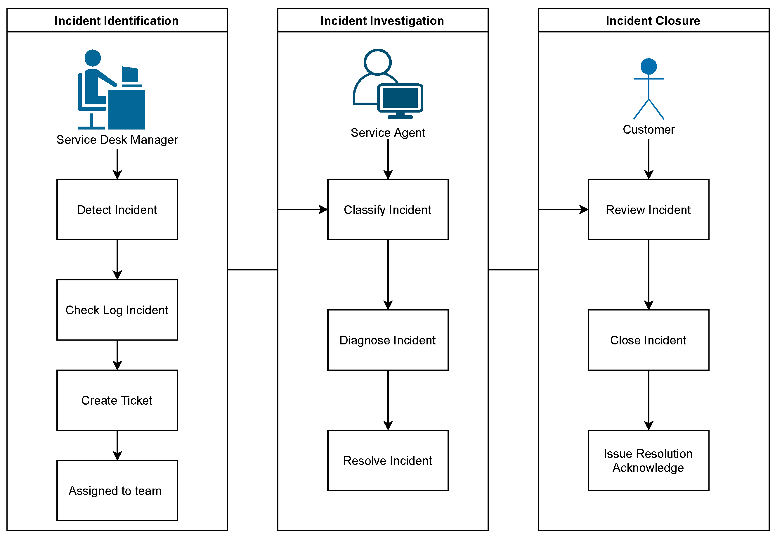
An example of a typical IT incident management system is presented in Figure 1.

In a typical manual process, the IT service desk is entirely responsible for managing major incidents, from the identification until the resolution and closure [5]. Due to its manual aspect, human errors directly impact the efficiency of the operation (e.g., wrongly assigned tickets resulting in more time to process and probable waste of resources) [6]. In addition, if too many incidents arise and a priority queue is activated, the severity assignment becomes critical, as wrongly prioritized incidents further increase the complexity of the problem. Ref. [7] identified that companies with a well-managed incident management system had managed to minimize their productivity losses and maintain their service quality. Therefore, incident prioritization was essential to determine the impact of such outages. Similarly, the ability to predict major incidents from the initial incident reports could provide a significant advantage in reducing disruptions and preventing actual outages from occurring. However, this is not a straightforward process, and there are some issues to address:

• Multi-modal Unstructured Data: Incident reports often contain text and numerical information.
• Mixing Data: Incident reports with similar content could be linked to a significant outage or only a minor problem.
• Imbalanced Data: Many incident reports are often related to minor incidents, rather than major incidents.

1.1. Scope and Problem Definition

The incident management process begins as soon as incident ticket logs have been generated. Most of the time, these outages resolve at the organizational level (depending on the system’s availability) or via the system’s components (specific system segments issue an alert). Based on the severity of the issue, the tickets are then forwarded to the relevant subject matter experts. However, the IT service management (ITSM) process is still manual, which results in inaccuracies and financial losses (e.g., backlogs due to miss-assignment of severity, high disc-memory usage, time consumption for root-cause analysis). AIOPS addressed problems by classifying outages and responding appropriately to the situation. AI was employed to do this. AIOPS real-world difficulties and threats were reflected in the statistics from the IT outage incidents. This information was kept private. It operated optimally with a three-tier architecture that incorporated system, data, and management tools.

1.2. Contributions

In this paper, we have provided a framework for proactive incident risk prediction. This framework describes a learning value to the company, prevents and mitigates risk, and optimizes resources with improved customer service and satisfaction.

• We proposed a novel framework for automating the prediction of major incidents to mitigate risks associated with the escalation of incidents. We aimed to transform reactive major incident management to proactive, within IT infrastructure.
• We presented different possible solutions to handle the imbalances in the major incident report (MIR) and non-major incident report (NMIR) records in the dataset.
• We then conducted a comparative analysis of state-of-art classification models designed to predict major IT incidents.

The organization’s primary aim should govern IT risk management [8]. Risk mitigation should include immediate responses, appropriate improvements, and continual risk monitoring [9]. Given the widespread usage of AI in numerous business sectors, our working hypothesis was that IT incident management should be automated. We provided an automated service management system based on cutting-edge AI models, such as machine learning (ML) and deep learning (DL). Large organizations can use this approach to enable early event detection and prioritization.

The rest of the paper is organized as follows: Section 2 provides the literature review, Section 3 describes the data, followed by Section 4, which proposes a novel framework for incident risk prediction with the state-of-the-art classification method description. Section 5 describes the experimental setup, and Section 6 provides the results and analysis. Finally, Section 7 discusses the research. A conclusion is provided in Section 8.

2. Background

There has been limited implementation of ML techniques that are specific to IT incident classification. A summary of recent studies is listed in Table 1. From our observation, among the prominent works adopting conventional ML classifiers for IT incidents, support vector machine (SVM) has been the most popular (22 studies), followed by naive Bayes (NB) with 13 studies, decision tree (DT) with 10 studies, k-nearest neighbor (KNN) with 5 studies, logistic regression (LR) with 4 studies, and lastly, only 2 studies implementing random forest (RF). Large-scale organizations opted for the simplicity of these conventional ML models due to their limited resources in terms of organizational structures and computing facilities. For example, SVM was preferred simply because the algorithm is less computationally demanding and, thus, significantly reduces the cost of the solution.

In addition, there has been a lackluster interest in adopting DL network models for IT incident classification, which is a stark contrast to the popularity of these models in most other industries. One potential problem has been the implementation complexity, particularly the interpretive ability of the algorithms and the computational resources demanded when training DL models. There have been very few implementations of DL available in the literature, and only [10,11] using long short-term memory networks (LSTM) [12] and convolutional neural networks (CNN) [13] were noted. As expected, the implementation of a more advanced method (e.g., deep transfer learning transformers such as bidirectional encoder representations from transformers (BERT) [14], robustly optimized BERT (RoBERTa) [15], and enhanced representation through knowledge integration (ERNIE 2.0) [16]) was even rarer. We found a single study by [17] that adopted BERT in their IT incidents risk prediction model. Independent of the underlying algorithms, most DL models require a precise set of parameters that have been tailored to the problem. These parameters are frequently static and often hard-coded into the models. As such, updating and maintaining these solutions is complicated and requires a dedicated team [18]. More advanced DL models have been synonymous with black boxes, which are relatively complex to interpret. Due to this high level of abstraction, many firms may be reluctant to trust the output generated from DL models, which could result in the failure of automation initiatives.

Understanding the semantics of IT incidents is essential for building the overall context of the corpus. The incidents in their raw form contain quality and usability constraints that must be removed using natural language processing (NLP) and preprocessing approaches [19]. Critically, when considering the imbalanced distribution often associated with real-time datasets, researchers have overlooked critical features when developing their corpus. We examined the existing NLP preprocessing pipelines and observed some interesting challenges, including the implementation of lemmatization and stemming strategies during the preprocessing phase. Previous analyses have revealed that language modeling techniques have produced better results for lemmatization than for stemming for document retrieval when precision was the performance metric. Another study by [17] addressed the issue of identifying the right textual features for a large corpus using a tailored preprocessing pipeline. However, the pipeline was not generic and required substantial changes, based on the specific attributes of the datasets, to function. Despite the complexity of context understanding, NLP techniques have been developed for feature extraction (as listed in Table 1) to capture the maximum attributes of a given corpus.

In terms of the specific feature-engineering techniques, the term frequency-inverse document frequency (TF-IDF) [20] has been the most preferred (12 implementations for incident severity prediction studies were found). TFIDF has been preferred because TF-IDF vectorization determines the TF-IDF score for each word in the corpus and assigns that information to a vector. As a result, each document in the corpus had its own vector, and the vector had a TF-IDF score assigned to every word that appeared anywhere in the collection of documents at any time. The vector detected whether or not two texts were comparable by comparing their TF-IDF vectors using a cosine similarity metric. TF-IDF provides a simple way to calculate the association between features and their importance within a text. It is memory and operationally efficient, which contributes to its popularity. Another popular approach has been the count vectorizer, a traditional feature extraction method based on the bag-of-words approach [21]. As compared to TF-IDF, count vectorizer was more computationally intensive and often unable to identify important keywords [22]. Despite the popularity of both methods, there have been clear limitations, especially when handling large-scale, unstructured, and imbalanced datasets commonly found in IT incident reporting.

Conventional ML vectorizers have a limited vocabulary, which is insufficient for large datasets. As indicated in [21], conventional vectorizers were ineffective in handling real-world ITSM data because they could not be upgraded. The vocabulary of traditional ML approaches was fixed and unable to adapt to upcoming real-time tickets. Most conventional vectorizers are also costly due to the cardinality review that must be performed exhaustively for each word. These weaknesses have been addressed by adopting a more advanced feature extraction method offered by state-of-the-art models, such as BERT, RoBERTa, and ERNIE 2.0. These Transformer models can avoid repetition, providing positional embeddings and learning relationships between words. For example, ref. [17] presented results showing transformer-based feature extractors outperformed conventional vectorizers.

The survey presented here revealed that in terms of performance when using accuracy as a metric, conventional ML models performed much better than the more advanced DL models. For example, [10], in their analysis using an open IT support ticket dataset, showed that NB outperformed the more advanced LSTM model (74% to 69% accuracy, respectively). Moreover, ref. [12] demonstrated a gradient boosting (GB) model that slightly outperformed a CNN model by 3% with an accuracy score of 95%–92% for automating the Information Technology Infrastructure Library (ITIL) dataset. On the contrary, we found this was not reflective of the true potential of these advanced DL models. There have been noteworthy issues in their implementations, such as insufficient training due to limited infrastructure (most advanced DL methods require extensive training to facilitate learning [23]), lack of understanding of the DL architecture (difficult to identify the bias of the model), lack of hyperparameter optimization (which is time-consuming and requires extensive memory utilization), and lack of validation for performance evaluation.

In this literature survey, we recognized that an updated comparative analysis of ML algorithms and state-of-the-art DL approaches, including transformer architectures for incident prediction, was required, as the vocabulary handled by ML classifiers is limited, making ML insufficient when learning from larger datasets that are complex (mixed and unstructured) and imbalanced. Therefore, we present a comprehensive analysis in this paper, focused on first-time transformer models. We hypothesized that the transformer model could significantly improve performance metrics due to its attention mechanism and its ability to handle larger vocabulary sizes.

Table 1. Existing implementations of automated IT incident prediction utilizing AI models.

Data	Pre-Processing	Feature Engineering	Techniques	Ref
Open-source data of Endava helpdesk operators	anonymization, lowercasing, lemmatizing, stemming, noise removal	No	CNN, RF, GB, average and stack ensemble	[24]
ITIL CHM department	removing stop words, punctuation, turning to lowercase, stemming	linguistic Features	TF-IDF and KNN, decision tree, NB, LR, SVM, QUICKSUCCESS	[25]
Fast-food restaurant chain	DateTime column named closed ticket transform from string to DateTime format.	feature extraction was performed based on daily data. Irrelevant features were removed. The feature was selected based on probability theory.	NB, LR, and gradient boosting decision tree model	[26]
IT department from a big multinational company	tokenization, stop word and digits removal, word stemming, and part-of-speech filtering by selecting only open grammatical classes	word count per solution category against text data.	TF-IDF and multinomial naive Bayes SVM, KNN, decision tree, and logistic regression	[27]
IBM Tivoli monitoring system	No	No	HMDB and ICTR model	[28]
German Jordanian University.	remove HTML tags and special characters	TF-IDF feature vectorization	SVM, NB, rule-based, and decision tree	[29]
IT infrastructural incident data	remove stop words, special characters, date and time, phone number, and email address	Chi-squared was used to select important features using TFIDF vectorizer. Top 1000 important feature selected.	NB, SVM, and Ada SVM	[30]
IBM CMDB dataset	keywords and their annotations as classification features	Selecting top Configuration Item records from CMDB to prevent complexity. TF-IDF was used to give importance	SVM	[31]
Incident issue tracking system of Istanbul Technical University data	purifying of tickets from HTML and numerical expression tags was carried out	Bag of words using TF-IDF	decision trees, SVM, KNN, and NB	[32]
Confidential data of IT Company	tokenization, stop words removal, and stemming	part of speech tagging was performed to filter out vocabulary	SVM	[19]
Real-world incident ticket data	tokenization, stop words removal and stemming	TFIDF	SVM	[33]
Real-world IT infrastructure service desk ticket data	remove stop words, special character, date and time, phone number, and email address	TF-IDF	LR, K-NN, MNB and SVM	[34]
Organization ticket data	lemmatization, POS tagging	TFIDF with Jaccard coefficient filtration	k-means clustering, Jaccard distance, and cosine distance	[35]
UCI ML repository	No	embedding	relational graph convolutional networks	[36]
Case study data	No	TFIDF	SVM using RBF kernel and XGBoost	[37]
IBM real-time dataset	HTML tag removal, Unicode inconsistencies, header/footer/entities replacement	semantic role sampling	BERT	[17]
Telco trouble ticket dataset	remove punctuation and stop words	TFIDF	random forest, DL, gradient boosting, XGBoost, and extremely randomized trees classifiers	[38]
Service Now dataset in IT help desk and ticketing	remove punctuation and stop words	Doc2vec using ServiceNow ticketing system	logistic regression	[18]
Tickets dataset of service level agreement	remove punctuation and stop words, URL.	Count Vectorizer	decision trees, SVM, KNN and NB	[39]

Table 1. Existing implementations of automated IT incident prediction utilizing AI models.

Data	Pre-Processing	Feature Engineering	Techniques	Ref
Open-source data of Endava helpdesk operators	anonymization, lowercasing, lemmatizing, stemming, noise removal	No	CNN, RF, GB, average and stack ensemble	[24]
ITIL CHM department	removing stop words, punctuation, turning to lowercase, stemming	linguistic Features	TF-IDF and KNN, decision tree, NB, LR, SVM, QUICKSUCCESS	[25]
Fast-food restaurant chain	DateTime column named closed ticket transform from string to DateTime format.	feature extraction was performed based on daily data. Irrelevant features were removed. The feature was selected based on probability theory.	NB, LR, and gradient boosting decision tree model	[26]
IT department from a big multinational company	tokenization, stop word and digits removal, word stemming, and part-of-speech filtering by selecting only open grammatical classes	word count per solution category against text data.	TF-IDF and multinomial naive Bayes SVM, KNN, decision tree, and logistic regression	[27]
IBM Tivoli monitoring system	No	No	HMDB and ICTR model	[28]
German Jordanian University.	remove HTML tags and special characters	TF-IDF feature vectorization	SVM, NB, rule-based, and decision tree	[29]
IT infrastructural incident data	remove stop words, special characters, date and time, phone number, and email address	Chi-squared was used to select important features using TFIDF vectorizer. Top 1000 important feature selected.	NB, SVM, and Ada SVM	[30]
IBM CMDB dataset	keywords and their annotations as classification features	Selecting top Configuration Item records from CMDB to prevent complexity. TF-IDF was used to give importance	SVM	[31]
Incident issue tracking system of Istanbul Technical University data	purifying of tickets from HTML and numerical expression tags was carried out	Bag of words using TF-IDF	decision trees, SVM, KNN, and NB	[32]
Confidential data of IT Company	tokenization, stop words removal, and stemming	part of speech tagging was performed to filter out vocabulary	SVM	[19]
Real-world incident ticket data	tokenization, stop words removal and stemming	TFIDF	SVM	[33]
Real-world IT infrastructure service desk ticket data	remove stop words, special character, date and time, phone number, and email address	TF-IDF	LR, K-NN, MNB and SVM	[34]
Organization ticket data	lemmatization, POS tagging	TFIDF with Jaccard coefficient filtration	k-means clustering, Jaccard distance, and cosine distance	[35]
UCI ML repository	No	embedding	relational graph convolutional networks	[36]
Case study data	No	TFIDF	SVM using RBF kernel and XGBoost	[37]
IBM real-time dataset	HTML tag removal, Unicode inconsistencies, header/footer/entities replacement	semantic role sampling	BERT	[17]
Telco trouble ticket dataset	remove punctuation and stop words	TFIDF	random forest, DL, gradient boosting, XGBoost, and extremely randomized trees classifiers	[38]
Service Now dataset in IT help desk and ticketing	remove punctuation and stop words	Doc2vec using ServiceNow ticketing system	logistic regression	[18]
Tickets dataset of service level agreement	remove punctuation and stop words, URL.	Count Vectorizer	decision trees, SVM, KNN and NB	[39]

3. Dataset Description

For this study, we used a dataset from a large multinational company comprising 500,000 total records. The dataset comprised real-time IT incidents collected from January 2020 to March 2021. These incidents were recorded by the organization’s three main stakeholders (agencies, employees, and customers). The reported incidents were classified either as major incident reports (MIR) or non-major incident reports (NMIR). Examples of the incident reports are provided below:

• MIR: “Why am I unable to print from any application? All staff is unable to print. No error message.”
• Non-MIR: “How do I update Java? Outlook web version running slow.”

An MIR was an incident report that had been escalated to major status or had a direct link to major incidents identified by the IT team. Conversely, NMIR was a regular incident with less impact on the operation. The class of each incident was labeled retrospectively after processing. The dataset is structured as:

$$Agency\_records=\sum Agency\left(\mathbf{MIR},\mathbf{NMIR}\right),$$

$$Employee\_records=\sum Employee\left(\mathbf{MIR},\mathbf{NMIR}\right),$$

$$Customer\_records=\sum Customer\left(\mathbf{MIR},\mathbf{NMIR}\right)$$

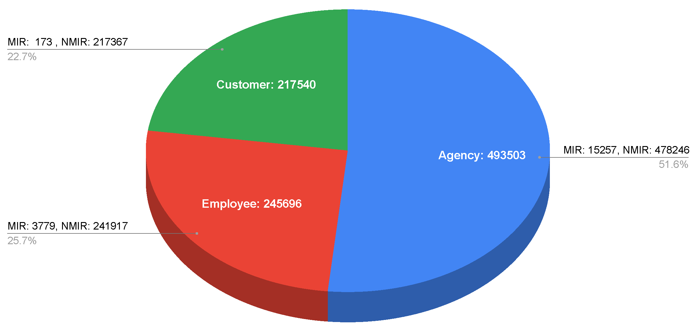
The distribution of the datasets is depicted in Figure 2. The Agency_records contained 493,503 incidents, out of which 15,257 were MIR and 478,246 were NMIR records. The Employee_records contained 245,696 incidents with 3779 MIR and 241,917 NMIR values. The Customer_records had 217,540 incidents with 173 as MIR and 217,367 as NMIR. As observed, the datasets were significantly imbalanced and skewed heavily in favor of NMIR incidents.

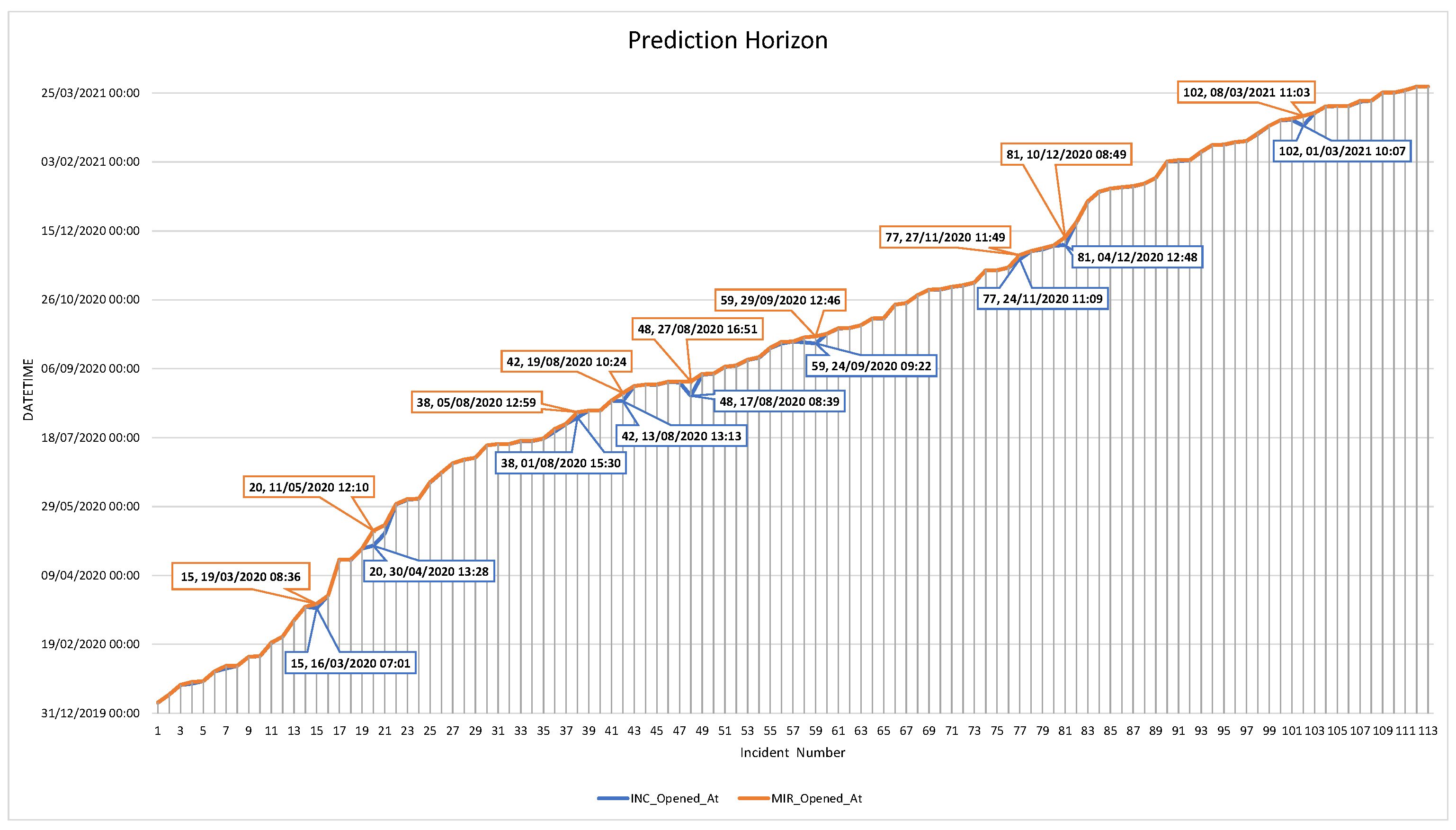
Specific to this study, we only used the Description, Short description (incident details), and the Status (labels MIR or NMIR) within the available datasets columns. In addition, we utilized the MIR opened at (MOA) and Incident opened at (IOA) columns for estimating the prediction horizon (i.e., time advantage that could be realized by investigating the cause of an incident potentially related to a major outage). A sample of the dataset is described in

Table 2. Data dictionary.

Column ID	Description	Values
Incident number	The unique internal code of the incident	INC123xxxx
Assignment group	The group to which the incident has been assigned.
Opened at	Date/Timestamp of when created the incident record.	17 March 2020
Closed at	Date/Timestamp of when the incident record was closed.	18 March 2020
Incident severity	The level of impact for each incident.	(1—High; 2—Medium; 3—Low; 4—None)
CMDB	The name of the configuration management database associated with the incident
Category	The category associated with the incident
Short description	Brief information about the incident.
Description	Detailed information about the incident.
Status	The manual mapping from problem to incident.	(0—MIR; 1—Non-MIR).
MIR opened at	Date/timestamp of when created the MIR record.	17 March 2020
Incident opened at	Date/timestamp of when the incident record was opened.	18 March 2020

. To address the imbalanced class issue in our dataset, we curated new datasets using a custom data-augmentation approach [40]. We added the actual MIR records from the other stakeholders’ datasets to each stakeholder dataset. This enriched each dataset while preventing additional extraneous information in the vocabulary. Data augmentation was intended to increase the occurrences of the MIR classified incidents that were severely lacking in the original dataset. The dataset composition was, as follows:

$$Agency\_resampled=\sum Agency\_records+\sum Employee\left(\mathbf{MIR}\right)+\sum Customer\left(\mathbf{MIR}\right),$$

$$Employee\_resampled=\sum Employee\_records+\sum Agency\left(\mathbf{MIR}\right)+\sum Customer\left(\mathbf{MIR}\right),$$

$$Customer\_resampled=\sum Customer\_records+\sum Employee\left(\mathbf{MIR}\right)+\sum Agency\left(\mathbf{MIR}\right)$$

We also concatenated all the records to increase the number of MIR records, as follows:

$$Combine\_All=\sum (Agency\_records+Employee\_records+Customer\_records)$$

We also performed up-sampling using the synthetic minority oversampling technique (SMOTE) [41]. We used SMOTE for oversampling because it generated synthetic data points that were different from the actual points instead of duplicating records with no extra information and increasing vector size. Using SMOTE, we generated three sampled subsets:

$$Agency\_smote=\sum SMOTE\left(Agency\left(\mathbf{MIR},\mathbf{NMIR}\right)\right),$$

$$Employee\_smote=\sum SMOTE\left(Employee\left(\mathbf{MIR},\mathbf{NMIR}\right)\right),$$

$$Customer\_smote=\sum SMOTE\left(Customer\left(\mathbf{MIR},\mathbf{NMIR}\right)\right)$$

Our literature survey indicated that most of the reported studies did not use resampling, which may have resulted in sub-optimal learning [19,29,37]. We hypothesized that by increasing the minority class (i.e., in the highly imbalanced situations observed in our dataset), we could improve the feature extraction of the minority class (in this case, MIR classified reports), which would lead to a higher accuracy. By performing SMOTE, we managed to increase occurrences of the minority class (MIR) records. For Agency_smote, we generated 462,989 MIR records, which were added to the existing 478,246 NMIR records. For Employee_smote, we generated 238,138 MIR records, which were added to the existing 241,917 NMIR records. For Customer_smote, we generated 217,194 MIR records, which were added to the existing 217,367 NMIR records.

4. Proposed Framework

Currently, there is a gap in the literature concerning the performance evaluation of AI algorithms in this domain. In this study, we proposed a comprehensive framework that compared various ML and DL approaches, specifically for IT incident prediction, using our proprietary industry-level data. We developed a computational pipeline that began with preprocessing, followed by feature extraction, training, and evaluation (a detailed description of the pipeline is presented in Section 5.1) and shown in Figure 3.

Our comparative pipeline is shown in Figure 4. The first phase of the pipeline was data preparation. As discussed earlier in Section 3, we had performed data augmentation and synthetic resampling on our original dataset. These datasets were split (70% for training and 30% for testing). Using the training data, we had performed supervised training using all 11 classifiers. Specific to the DL-based classifiers, we allocated 20% of our training dataset for training validation using the default Keras model’s fit function. The training phase was performed for 10 epochs with binary_crossentropy as the loss function and AUC as the performance metric. We selected AUC as a metric to prevent over-fitting due to the imbalanced characteristics of our dataset. Finally, the models were tested with the test data (30% of the dataset). Similarly, the AUC score was determined to evaluate the performance of all 11 classifiers.

An essential element of the prediction framework was the utilization of various state-of-the-art classifiers. In this work, we categorized these classifiers as (1) conventional ML methods, including NB, SVM, gradient boosting (GB), extreme gradient boosting (XGBoost), and categorical boosting (CatBoost); (2) DL-based approaches, including gated recurrent unit (GRU), CNN, and Bi-LSTM; and lastly, (3) transformers, including BERT, robustly optimized BERT (RoBERTa), and enhanced representation through knowledge integration (ERNIE 2.0). A brief description of each classifier is provided below.

• NB [42]: Naive Bayes classifier is based on Bayes theorem and is one of the popular ML algorithms for classification. NB is a simple probabilistic model that assumes that each feature or variable of the same class makes an independent and equal contribution to the outcome. Our dataset was divided into a feature matrix and a target vector. The feature matrix (X) contained all the vectors (rows) of the dataset, in which each vector consisted of the value of dependent features. We assumed that the number of features were d, $X=(x_1,x_2,x_3,\dots ,x_d)$ while the target vector (y) contained the value of the class variable for each row, according to its feature matrix. The feature matrix (X) was the incident description reported in the database system. The target (y) value would either be MIR or NMIR. In this instance, $P\left(y\right|X)$ was the probability of the class y (for MIR or NMIR), according to the incident description (X). The maximum probability function provided the classification label, either MIR or NMIR.
• GB [43]: Gradient boosting classifier is an approach developed to train a weak hypothesis iteratively to arrive at a better hypothesis. Gradient boosting combines the previous model with the next generated model to minimize the prediction error. It minimizes the loss function iteratively, starting with a negative gradient, i.e., a weak hypothesis. In this work, we performed a binary classification (MIR or NMIR) using the description column of the incident. The algorithm began with one leaf node that predicted the initial value for each description of the incident. Next, the algorithm used the $log\left(odds\right)$ of the target value, yielding an average survival value assigned to our initial leaf node. If the probability of surviving exceeded $0.5$, we first classified every sample in the training dataset as MIR. (Note: where $0.5$ was a common threshold value associated with binary classification decision based on probability).
• XGBoost [44]: Extreme gradient boosting is an optimized GB technique that provides efficient, flexible, and portable tree model results. It offers parallel tree boosting that provides solutions quickly and accurately. XGBoost is efficient for open-source implementation and significantly distributed environments, such as Hadoop, Sun Grid Engine (SGE), and Message Passing Interface (MPI). It predicts the residual or error of prior models to obtain its final predictions. The gradient descent algorithm minimizes loss when adding new models. We trained the model with 500 trees and a depth (max_depth) of 1 (for the root node). As compared to other available boosting techniques, e.g., GB, XGBoost was fast, memory efficient, and highly accurate [45].
• Catboost [46]: Category and boosting adopts minimal variance sampling, a type of stochastic gradient boosting with weighted sampling. In this instance, the weighted sampling occurred at the tree level and not the split level. It grows as a balanced tree; the split score minimizes the loss and maximizes the accuracy score. Changing policy parameters (with a penalty function at level nodes) is also possible. In contrast to a traditional approach, this study addressed the MIR and NMIR classification problems. We trained the model with 400 trees and a depth (max_depth) of 1 (root node only). As compared to the XGBoost, Catboost was twice as fast with better accuracy [47].
• SVM [48]: Support vector machines utilize associated learning to analyze data for classification. Based on the descriptions of known incidents, SVM built a model that assigned MIR or NMIR labels to new incidents. The algorithm considered all incident descriptions and mapped them to a space that maximized the distance between the two classes. In the context of this study, we had a training dataset of incident descriptions labeled “0” for MIR and “1” for NMIR, $(x_1,y_1)\dots (x_n,y_n)$ where $y_i$ is either 0 or 1, each denoting to a point $x_i$, where each $x_i$ is a p-dimensional real vector. We were interested in the maximum-margin hyperplane that divided the group of points $x_i$, for which $y_i=0$ from the group of points for which $y_i=1$, which was defined so that the distance between the hyperplane and the nearest point $x_i$ from either group was maximized. Any hyperplane could be written as the set of points x, satisfying $w^T\mathbf{x}-b=0$, where w was the (not necessarily normalized) normal vector to the hyperplane. This was similar to Hesse’s normal form, except that w was not necessarily a unit vector. The parameter $\frac{b}{\parallel \mathbf{w}\parallel }$ determined the offset of the hyperplane from the origin along the normal vector W.
• Bi-LSTM [49]: Bi-directional long short-term memory is an improved version of the LSTM model (a variant of the recursive DL architecture) that can process data in both forward and backward directions. Bi-LSTM helps map models that allow for sequential dependencies in words and phrases. For our framework, Bi-LSTM assisted in training MIR and NMIR sequences by preserving this information using two independent RNN cells that stored the iterative states for a longer time. Bi-LSTM contained the IT incident input $\left(X_t\right)$ concatenated with hidden state $(h_t-1)$, which was further forwarded to three gates (Forget, Input, and Output). The Input gate has an embedded gate known as an Update. The Update gate memorized the past and present sentence sequence. The value from the update gate multiplied the cell state $(C_t-1)$, resulting in the hidden state or unit $\left(h_t\right)$. Our Bi-LSTM architecture comprised five layers: one embedding layer with a size of 300, one bi-directional layer with 280 LSTM neurons, two dropout layers, and one classification layer (dense layer). The total number of trainable parameters for the model was 23,346,401.
• CNN [50]: Convolutional neural network is synonymous with image classification, but recently, it has significantly contributed to NLP. CNN is used to extract high-level feature functions from n-gram. For example, ref. [51] developed a word-embedding matrix layer that memorized the weights during the network training phase. We used our framework’s input labels (MIR or NMIR) as tokens to map to the word-embedding matrix. In this mapping, every convolutional filter mapped to each window of the embedding layer. In CNN, matrix reduction reduced the dimension of the matrix to a constant length. We executed the matrix reduction on every possible window. Each reduced matrix was the input for the fully connected layer. In the next layer, we used the activation function to create a single dimension input of features per tensor output; The global max pooling layer with 256 batch sizes and 23,027,144 trainable parameters were used. In the final layer, we applied the Softmax activation function to translate the real-probability values into MIR or NMIR labels.
• GRU [52]: Gated recurrent unit is an RNN DL variant that retains information for a longer time and improves the computing speed. GRU consists of two neural gates (Update and Reset gates) for updating the previous cell state and discarding the irrelevant state. For this purpose, we provided MIR or NMIR values as input $X_t$, which concatenated with hidden states $H_{t-1}$ and moved to the Update gate. In the final phase, we used the Sigmoid activation function to maintain an output within the range of (0,1), resulting in an MIR or NMIR value. The architecture comprised 5 layers, containing one embedding layer with a size of 300 vectors, one GRU layer with 140 neurons, and one dense layer with a sigmoid activation function. The model had a total of 23,037,981 trainable parameters.
• BERT [14]: Bidirectional encoder representations from transformers consists of several encoder transformers within a pool of pre-trained models. BERT follows the bidirectional orientation of learning information from a sequence of words from left to right and right to left. Each encoder encapsulates two sub-layers: a self-attention layer and a feed-forward layer. We have employed a trained BERT architecture contain 12 layers of the encoder, 12 attention heads, 768 hidden sizes, and 110M trainable parameters. It was pre-trained on 800M unlabeled data extracted from BooksCorpus and 2500 M words from Wikipedia, and then, it was transferred to the incident prediction problem. We performed an additional preprocessing step for our dataset using the BERTtokenizer. It tokenized and reformatted the sequence of tokens by adding CLS (a classification token indicating the start of a sequence) and SEP tokens (appended to the end of the sequence). The length of our incident description token was less than 512 tokens; therefore, we utilized padding (PAD) to fill the unused token slots (further details below). Our BERT model output an embedding vector of 768 in each of the tokens and had 340M trainable parameters.
• ERNIE 2.0 [16]: Enhanced Representation through knowledge Integration (ERNIE) is a pre-trained framework that performs the training of new sequences with historically trained tasks. For text classification, ERNIE 2.0 has outperformed BERT with highly accurate results [16]. ERNIE 2.0 captures the contextual information with a series of shared text encoding layers, customized with recurrent neural networks or deep transformers with a stacked self-attention layer. Its multi-task learning encodes lexical, syntactic, and semantic information across tasks. When a new task arrives, this framework can incrementally train the distributed representations without forgetting the previously trained parameters. In our framework, we used 12 layers, 12 self-attention heads, and 768 dimensions in the hidden layer, resulting in 94M trainable parameters.
• RoBERTa [15]: Robustly optimized BERT emphasizes data being used for pre-training and the number of passes for training. The RoBERTa architecture was proposed to overcome the drawback of the original BERT model by increasing batch size from 256 to 8k, providing better speed for performance metrics [15]. We used a pre-trained transformer with built-in (vocab) 160GB in size for RoBERTa to conserve our computational resources. It reduced the perplexity of the masked language model by providing the provision to train with larger batches and longer sequences. It also provided the dynamic masking pattern over the training data during data preprocessing. In our framework, we implemented a large RoBERTa model with 12 encoder layers, 12 attention heads, and 768 dimensions in the hidden layer, resulting in 110M trainable parameters.

Finally, if an incident was classified as NMIR, it was assigned to the normal priority queue. If an incident was classified as MIR, it was directed to the high-priority queue and assigned immediately to the incident processing acceleration teams in order to resolve the issue as soon as possible.

5. Experimental Setup

We conducted the empirical analysis using the state-of-art for the proposed IT incident prediction framework. We evaluate our generated results with the off-the-shelf models described in Section 4. We performed preprocessing, as described in Section 5.1, and an analysis of the tokenizers, as described in Section 5.2. We reported our training in Section 5.3 and validation in Section 5.4.

5.1. Pre-Processing

Data preparation is critical in any text classification task. For this study, the incident descriptions in our datasets were highly unstructured with no specific formatting (i.e., entirely dependent on the user’s view). Therefore, we developed a preprocessing pipeline to standardize the input text and remove unnecessary noise. We started with the noise entity removal for HTML tags, stop words, punctuation, white-spaces, and URLs. Next, we normalized the data using the standard NLTK toolkit [53]. During the normalization, we performed tokenization, lemmatization, stemming, and sentence segmentation. For punctuation removal, we used a regular expression, in which we removed all the values other than alphabetic words (i.e., command r’[A-Za-z]’), then converted all the words into lowercase representations. We assigned these lower-case words as tokens using WordPunctTokenizer. The function tokenized a text into a sequence of alphabetic and non-alphabetic characters following regexp. Unnecessary white spaces, which were the byproducts of the upper-to-lower-case conversion, were removed. Lastly, manual cleaning of these sequences using the join and strip functions was performed. The resulting datasets were split as follows: 70% for training and 30% for testing. For training, we further split the training dataset by reserving 20% of the training dataset (from 70% of the original portion) for validation (which is necessary for DL-based models).

5.2. Tokenizer

Determining the separability between the MIR and NMIR incidents was key in our framework. Therefore, to enable a good generalization between the incident texts and their classes, we had to identify the vocabulary present in the datasets. To do so, we optimized the size of each token (i.e., the set of sub-words representing the vocabulary) as 35 words max_length. Tokenization allowed us to understand the differences between classes, analyze and compare vocabulary between datasets and identify any correlations within each class with accuracy. For DL-based models, we used the Keras tokenizer, and for the transformers, we used the BERTtokenizer, the RoBERTa tokenizer, and the ERNIE 2.0 tokenizer, which were compatible with the selected models. The resulting data after tokenization had various lengths. To mitigate this issue, we padded the data by adding zeros to reach a specific length (35) in order to ensure all the feature vectors had the same dimensions.

5.3. Training

For the ML models, we used TF-IDF for feature extraction. TF-IDF operated by extracting the essential words within the corpus, where TF was the term frequency of the words appearing in the ITSM corpus (all incident records in the training set), and IDF was the frequency of the datasets containing those words. The fewer words that appeared in the corpus, the higher the TF-IDF value would be. We used the sklearn library for our analysis to calculate the TF-IDF value. After the feature extraction via the TF-IDF vectorizer, we used the default settings for all conventional ML classifiers, as described in sklearn library [20] for training. The labels for every feature vector available from the raw data (MIR and NMIR) used the sklearn prediction function for evaluation.

For the DL models, the textual data were transformed into numbers and mapped to the embeddings to achieve better cardinality for each token. The first layer of our DL model was the embedding layer, consisting of three parameters: input dimension, input length, and output dimension). The next layer, called the model layer, contained hidden neurons that helped to model the complex data. It contained two parameters (the number of neurons and the return sequence). Finally, we used a dense layer with parameters such as input shape, batch size, and sigmoid as the activation functions. This layer was also known as the classification layer because it classified the output as MIR and non-MIR values. Compiling a model required parameters such as optimizer and loss function. We used the Adam optimizer and binary cross-entropy as loss functions. For the transformers, we used pre-trained transformers, from which we had already converted the incident reports from the training, validation, and test datasets to integer sequences at a length of 35 tokens each. Next, we converted the integer sequences to tensors. We created dataloaders for both training and validation sets. This dataloaders passed batches of training and validation data as input to the model during the training phase. We implemented the default configurations for BERT, ERNIE 2.0, and RoBERTa. The Figure 5 shows the architecture of our best performing transformer architecture.

5.4. Validation

To validate our results, we performed cross-validation, an approach that tests the performance efficiency of a model. In essence, the higher the performance metrics score for cross-validation is, the lesser the error associated with the model should be. We chose the sklearn stratified k-fold cross-validation because it is a refined form of the traditional k-fold cross-validation technique. It randomly divided the corpus so that the target class ratio in each fold remained at the same level as in the overall dataset, so the analysis results were consistent. This ensured that the minority class had sufficient samples during training and testing; we segmented the data ($Combine\_All$) into 5 folds. As an additional step, we ensured that the subsets for train and testing did not overlap. The system configuration is shown in

Table 3. Selected Parameters.

Classifier	Vocab_Size	Max_Features	Embedding_dim	Batch_Size	Filters	Kernel	Activation	Loss	Optimizer	Learning_Rate
	(500, 1 k, 10 k, 20 k, 30 k, 50 k)	(5 k, 10 k, 50 k, 200 k)	(64, 128, 256, 512)	(8, 16, 64, 128, 256)	(200, 400, 600, 800)	(1, 2, 3, 4, None)	(Relu, Sigmoid, Gelu, Tanh)	(categorical crossentropy, crossentropy loss)	(Adam, AdamW)	(0.01, $1\times {10}^{-3}$, $1\times {10}^{-5}$)
CNN	10,000	1000	128	256	100	4	Relu	categorical crossenthropy	Adam	0.01
Bi-LSTM	10,000	1000	128	256	25	None	Sigmoid	categorical cross entropy	Adam	0.01
GRU	10,000	1000	128	256	128	3	Sigmoid	categorical cross entropy	Adam	$1\times {10}^{-3}$
Bert	30,522	3072	512	8	768	None	Gelu	cross entropy loss	AdamW	$1\times {10}^{-5}$
RoBERTa	50,000	3072	514	8	768	None	Gelu	cross entropy loss	AdamW	$1\times {10}^{-5}$
ERNIE	18,000	3072	256	8	768	None	Relu	cross entropy loss	AdamW	$1\times {10}^{-5}$

and

Table 4. System Configuration.

Configuration Name	Version
Tensorflow	2.8.0
Python	3.7.7
Jupyter notebook	6.2.0
GPU	Tesla P100-PCIE-12 GB
GPU Memory	12 GB HBM2
System Interface	PCI e 3.0 * 16
Power Consumption	250 w

.

6. Result and Analysis

We conducted empirical analysis using the state-of-art for the proposed IT incident prediction framework. We evaluated our generated results from off-the-shelf models, as described in Section 4. We provided analysis on the tokenizer in Section 6.1, reported our evaluation quantitatively in Section 6.2, cross-validation in Section 6.3, and mean time resolution in Section 6.4.

6.1. Tokenizer Analysis

Tokenization allowed us to determine the vocabulary within our datasets. Considering our original dataset’s size and understanding of the inter-dataset characteristics, we performed an individual analysis of each dataset, as presented in Figure 6. For Agency_records (Figure 6a), the maximum differences between classes were visible in the first 20 tokens, when comparing the average tokenizer values. This indicated a good separability between class means consistency during training and testing. We observed the average token value range in the Agency_records was lower than that of the Employee_records (Figure 6b), which also correlated with a higher variance in tokens for the Employee_records. Thus, Employee_records had a more varied vocabulary in their corpus. The max separability appeared to occur between the 5th and 15th tokenizer for the Agency_records and the Employee_records. Upon closer inspection, we observed a relative difference between class means for the Employee_records at approximately 23 tokens. The profiles were significantly different for the Customer_records (Figure 6c), which had a much smaller MIR class with only 112 MIR samples in the training set, as compared to the 65,000 samples for the NMIR. Consequently, the average token value varied widely for the minority class (in this case, MIR). Accordingly, the average tokenizer values for the NMIR class were much lower, indicating a smaller corpus.

6.2. Quantitative Evaluation

As compared to more common performance metrics (e.g., accuracy), AUC or ROC were more suited metrics imbalanced datasets because they helped to identify over-fitting [54]. Higher AUC or ROC values represented better separability between the MIR and NMIR classes. Figure 7 depicts the qualitative scores with ROC/AUC for the Agency_records, Employee_records, and Customer_records. The scores presented in Figure 7 were averaged across the Agency_records, Employee_records, and Customer_records. Transformer based models (BERT, RoBERTa, and ERNIE 2.0) and XGBoost performed best with a 93% ROC score for the Agency_records dataset. For the Employees_records and Customers_records, CNN performed best at 95% and 74% ROC. Overall, Catboost achieved minimum ROC scores of 69%, 50%, and 50%. This was expected as Catboost struggled in unknown categories and needed to build in-depth decision trees for high cardinality features [55].

As indicated in Section 3, our datasets were highly imbalanced. Therefore, we resampled our dataset and re-ran our prediction pipeline. The results are depicted in Figure 8. ERNIE 2.0 achieved a 95% ROC for Agency_resampled. BERT and ERNIE 2.0 achieved the highest scores, 97% for Employee_resampled and ERNIE 2.0 at 98% ROC for Customer_resampled. NB achieved 71%, 53%, 59%, and 54% ROC for the Agency_resampled, Employee_resampled, Customer_resampled and Combine_All, respectively, which was the lowest among all the classifiers. A recurring issue with the NB model was that with no occurrences of a class label and a particular attribute value, the frequency-based probability estimation would be zero. A large dataset was required for reliable predictions of each class’s probability.

We also experimented with our synthetic data curation (SMOTE). For the Agency_smote and the Employee_smote, XGBoost performed best with 94% and 86% ROC scores, respectively. GB performed best for the Customer_smote with an 85% ROC value. Figure 9 shows that the DL models (Bi-LSTM, GRU, CNN) performed relatively poorly on all the synthetic subsets. This was largely contributed to the synthetic data profile generated by the SMOTE technique. SMOTE created more extensive and less specific decision boundaries that increased the generalization capabilities of the ML classifiers, which were more suited for one-hot encoding. In contrast, DL models used tokenizers, causing extensive feature spaces in NLP and resulting in the DL models falling quickly into high sparse dimensions.

6.3. Cross Validation

To validate our findings, we utilized the Combine_All dataset. Initially, we segmented our dataset into 5 folds by ensuring that it did not contain any records from the training set. We then applied our comparative framework to iteratively train each algorithm on $k-1$ folds while using the remaining holdout fold as the testing set. All the transformer models performed the best, with 90% or more ROC scores at each fold. In contrast, NB performed the worst, with ROC score less than 60% (Figure 10). Our k-fold results showed that our findings in Figure 8 were consistent with comparative ROC values with the cross-validation runs.

In Figure 11, we provided the average ensemble count (average of predicted labels for all models) of all the three classes corresponding to conventional ML, DL-based, and transformers. Additionally, we also reported a confusion matrix to verify the true-positive (TP), true-negative (TN), false-negative (FN), and false-positive (FP) classes for each fold. For example, the average ensemble count was the actual MIR value versus the predicted value for each fold (from 1 to 5), i.e., the true-positive (TP). The confusion matrix for ML, DL, and Transformers are listed in

Table 5. The k-fold cross-validation with complete data (Combine_All as described in Section 3) segmented in into five folds. We split data into 80:20 splits for training and testing by ensuring the testing set did not contain any record from the training set. We applied ML models naive Bayes, gradient boosting, XGBoost, CatBoost and SVM.

	Naive Bayes				Gradient Boosting				XG Boost
$\mathit{k}$-fold	TP	TN	FN	FP	TP	TN	FN	FP	TP	TN	FN	FP
1	276	64,735	1455	3	1154	64,638	577	100	1322	64,623	409	115
2	271	64,659	1536	3	1166	64,584	641	78	1363	64,562	444	100
3	275	64,758	1432	3	1068	64,682	639	79	1272	64,636	435	125
4	267	64,732	1465	4	1112	64,644	620	92	1284	64,620	448	116
5	261	64,729	1469	8	1075	64,461	655	96	1286	64,606	444	131
Mean	270	64,722	1471	4	1115	64,601	626	89	1305	64,609	436	117
	CatBoosting				SVM
$\mathit{k}$-fold	TP	TN	FN	FP	TP	TN	FN	FP
1	1302	64,621	429	117	1370	64,635	361	103
2	1373	64,565	434	97	1407	64,570	400	92
3	1256	64,646	451	115	1301	64,666	406	95
4	1303	64,621	429	115	1355	64,624	377	112
5	1287	64,611	443	126	1304	64,634	426	103
Mean	1304	64,612	437	114	1347	64,625	394	101

and

Table 6. The k-fold cross-validation with all data (Combine_All as described in Section 3) segmented in into five folds. We split data into 80:20 splits for training and testing by ensuring the testing set did not contain any records from the training set. We applied transformers (BERT, RoBERTa and ERNIE 2.0) and DL algorithms (GRU, Bi-LSTM and CNN).

	GRU				Bi-LSTM				CNN
$\mathit{k}$-fold	TP	TN	FN	FP	TP	TN	FN	FP	TP	TN	FN	FP
1	1334	64,513	397	225	1251	64,588	480	150	1304	64,553	427	185
2	1328	64,537	497	125	1301	64,514	506	148	1403	64,392	404	270
3	1260	64,599	447	162	1238	64,652	469	109	1205	64,633	502	128
4	1205	64,643	527	93	1169	64,666	563	70	1189	64,632	543	104
5	1280	64,575	450	162	1278	64,584	452	153	1289	64,563	441	174
Mean	1281	64,573	460	153	1247	64,600	494	126	1278	64,554	463	172
	Bert				Roberta				ERNIE
$\mathit{k}$-fold	TP	TN	FN	FP	TP	TN	FN	FP	TP	TN	FN	FP
1	1437	64,590	294	148	1429	64,616	302	122	1430	64,603	301	135
2	1438	64,597	293	141	1539	64,508	268	154	1486	64,562	321	100
3	1423	64,623	284	138	1525	64,495	282	167	1395	64,641	312	120
4	1454	64,613	278	123	1428	64,592	304	144	1401	64,529	331	207
5	1411	64,602	319	135	1390	64,580	340	157	1394	64,632	336	105
Mean	1432	64,605	239	137	1462	64,558	299	148	1421	64,539	320	133

. For example, in k-fold, there were 1731 total MIR, whereas the average ML (i.e., the average of the predicted label of all the ML models) predicted 1172 TP MIRs, as well as 1468 TP MIRs for the DL-based and 1609 TP MIRs for the transformers. Similarly, for TNs, NB predicted the 64,722 TNs for ML. For DL, Bi-LSTM predicted 64,600 TNs, and for the transformers, BERT reported the highest 64,605 TNs values. For conventional ML, the average predicted value for all folds was 1153, with SVM having the highest share with 1499, which was lower than the predicted labels of 1731. The DL models showed better ensemble results with 1394 predicted labels for all folds, with CNN having the highest number of 1673 predicted labels. Transformers outperformed the conventional ML techniques with 1584 average predicted ensemble labels. RoBERTa performed best with 1693. Overall, the transformers models performed the best for the Combine_All datasets (Refer Figure 8).

Similar to the average ensemble count, RoBERTa correctly predicted 1462 TPs and 64,558 TNs, whereas NB performed worst by identifying only 270 TPs and 64,722 TNs.

6.4. Mean-Time Resolution

For the meantime-to-resolve, we used the MIR outage records because they contained the escalated incident records. To calculate meantime-to-resolve, two DateTime columns were used: Incident_Opened_at and MIR_Opened_at. We defined the meantime-to-resolve as the time recorded, starting when the incidents had been reported and then resolved by the outage team. The meantime-to-resolve ranged from minutes to hours. The evaluation of meantime-to-resolve was conducted using the prediction horizon, as follows:

$$Prediction\_Horizon=\sum T_{2n}-\sum T_{1n},$$

where $\sum T_{2n}$ denotes MIR opened at ($T_2,....T_{2n}$) and $\sum T_{1n}$ denotes incident opened at (IOA) incidents ($T_1,....T_{1n}$).

Our prediction horizon (meantime-to-resolve ) for MIR records from January 2020 to March 2021 is depicted in Figure 12. The blue line indicates the IOA records while the orange shows the MOA records. The IOA points (in orange) indicated the highest DateTime record where an incident log is generated. MOA denoted the point where we declared an incident as MIR. For example, ticket #20 had been reported to IOA on 30 April 2020 and labeled as MIR on 11 May 2020 by the outage team, so it took around 11 days to resolve this incident. Another ticket, #48, had been reported as IOA on 17 August 2020 and labeled as MIR on 27 August 2020, taking around ten days. In Figure 12, we noted that the orange line overlapped with the blue line, indicating the closing of the incident at the same instance. We predicted the average prediction horizon time of MIR as 4 days, 3 h, and 26 min, which could provide a significant advantage in addressing incidents and could prevent major incidents or outages.

To further investigate our evaluation, we refined the prediction horizon by selecting only escalated incident records with time durations of 6 h or less. The reason was to scrutinize results in the context of hours (removing outliers that took more than days to resolve) to better quantify the improved meantime-to-resolve for most incidents, if predicted correctly. The leftover incidents numbered 44 (see Figure 13). The orange line shows the MOA values, indicating the incident escalated time, whereas the blue line shows the IOA records. Incident #1 took a maximum of 5 h and 35 min to escalate; in contrast, incident #7 took 5 min to mark as a significant incident. The analyzed results based on a refined search showed us the average time to resolve an incident within 1 day was 2 h and 30 min.

7. Discussion

This study comprehensively evaluated AI classifiers using a real-world proprietary dataset. As observed, we faced a highly skewed distribution with almost a million records for NMIR and only 19,000 records for the MIR (which was only 2% of the overall dataset). The datasets were highly unstructured, which further complicated the data-preprocessing task. Our datasets consisted of raw incident reports/tickets. Therefore, most records contained typographical errors, misspellings, grammatical mistakes, and slang words. We also noticed that 6% of the incident log contained duplicate records, which did not provide any extra information and consumed additional memory resources during processing. We suggested removing these records because it introduced sparseness problems and increased the vector size. In a real-world setting, IT incident datasets require extensive cleaning using a closely monitored preprocessing pipeline to extract important linguistic features, which we included as part of the proposed prediction framework. Additionally, we demonstrated that data augmentation provided relatively better results than the synthetic data. We developed a custom approach of data augmentation, in which actual data from various channels (representing the minority label) were added to enrich the dataset belonging to the industry stakeholder. This enrichment was more beneficial than generating synthetic records to avoid duplication that added no additional information to the vocabulary.

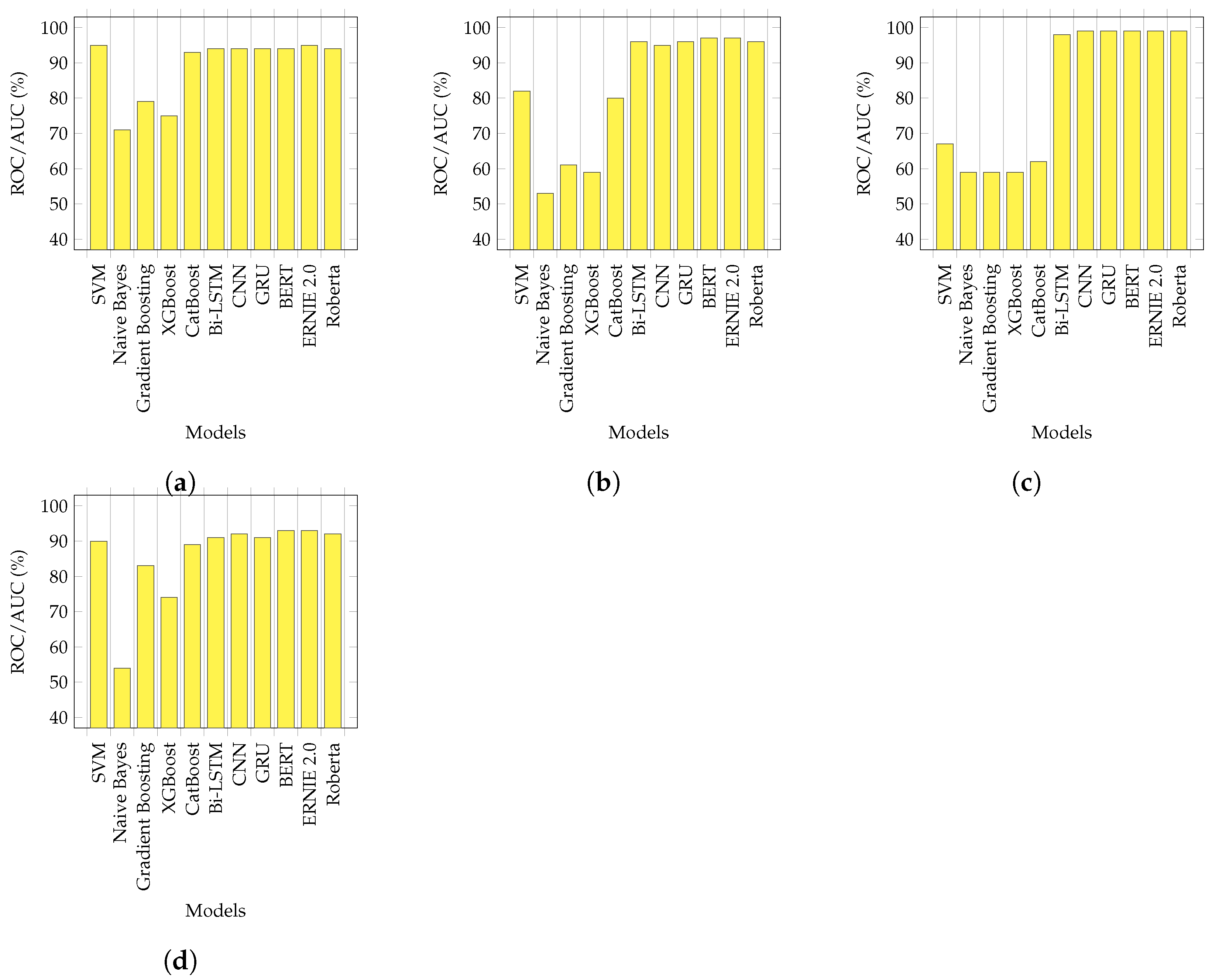
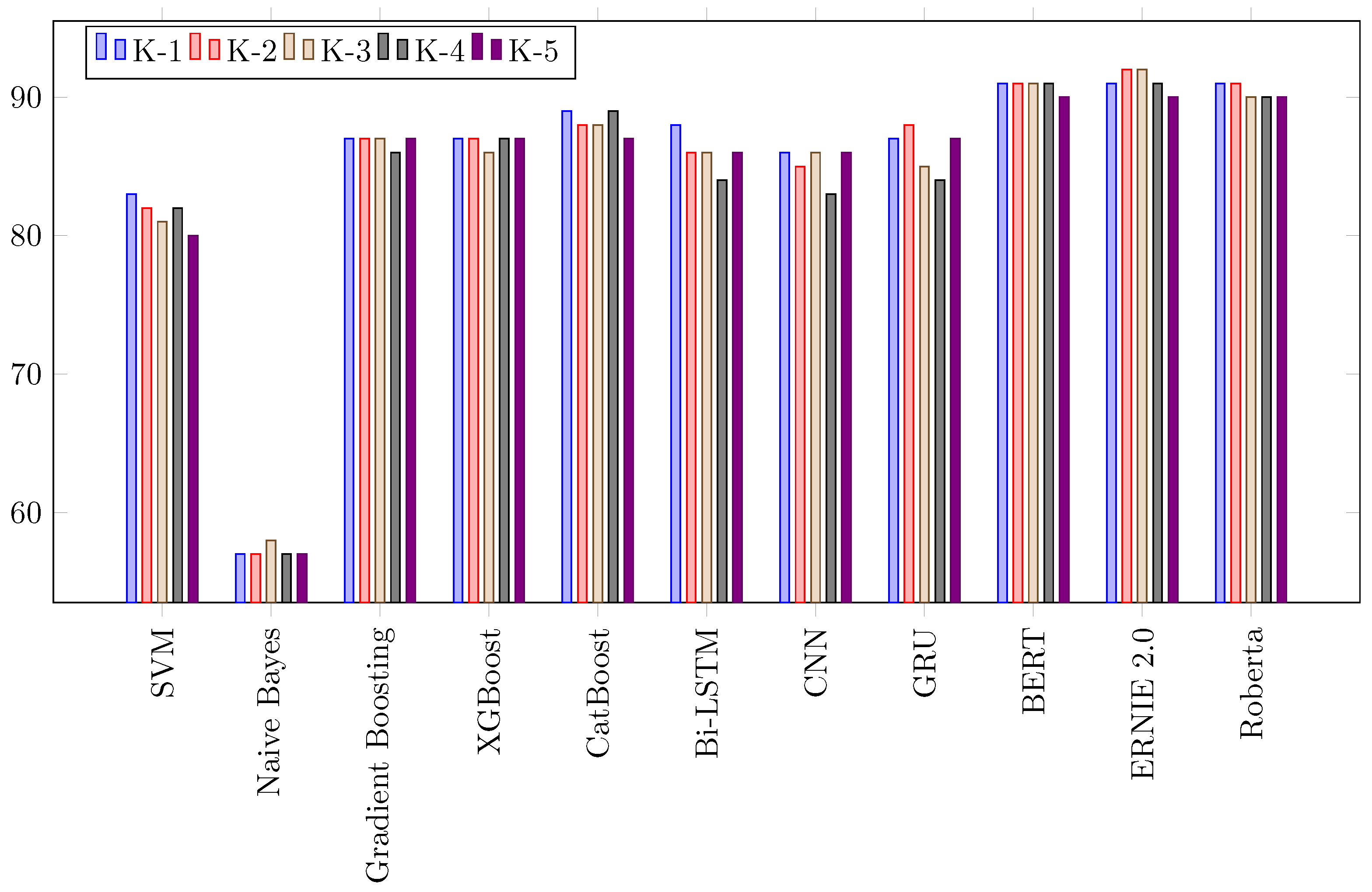
Our analysis showed that the transformers performed marginally better than the DL-based models and significantly better than the conventional ML models. For example, given the Combine_All dataset, ERNIE 2.0 outperformed all conventional ML models, performing better than NB, GB, SVM, XGBoost, and CatBoost, by 39%, 10%, 3%, 19%, and 4%, respectively. As compared to the DL-based models, ERNIE 2.0 produced slightly better results, with a 1% improvement over the CNN and a 2% improvement over the Bi-LSTM. Generally, the DL-based models performed better due to their recall memory units that extracted high-level abstract features; however, they performed slightly worse, as compared to transformers because of their limited vocabulary [10]. Our findings were in agreement with this observation.

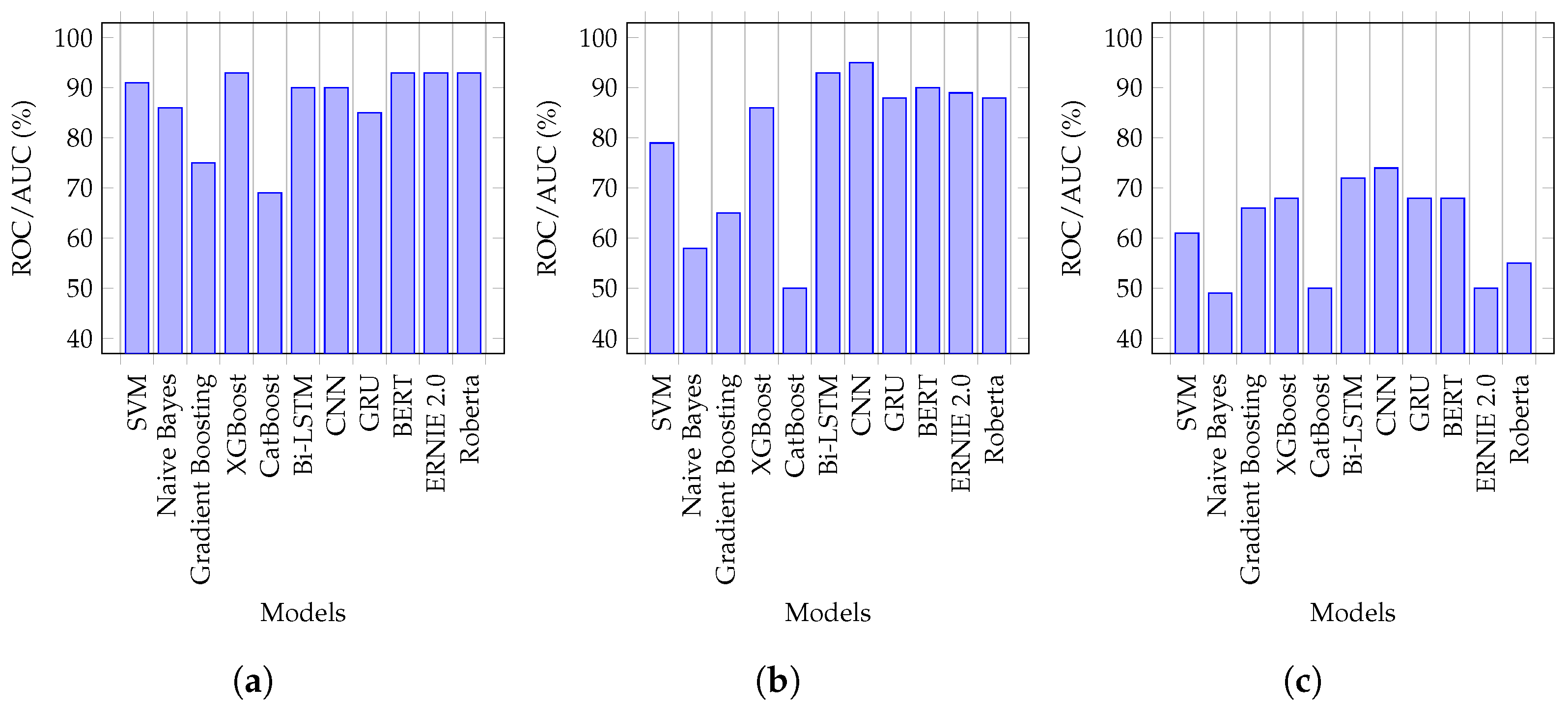
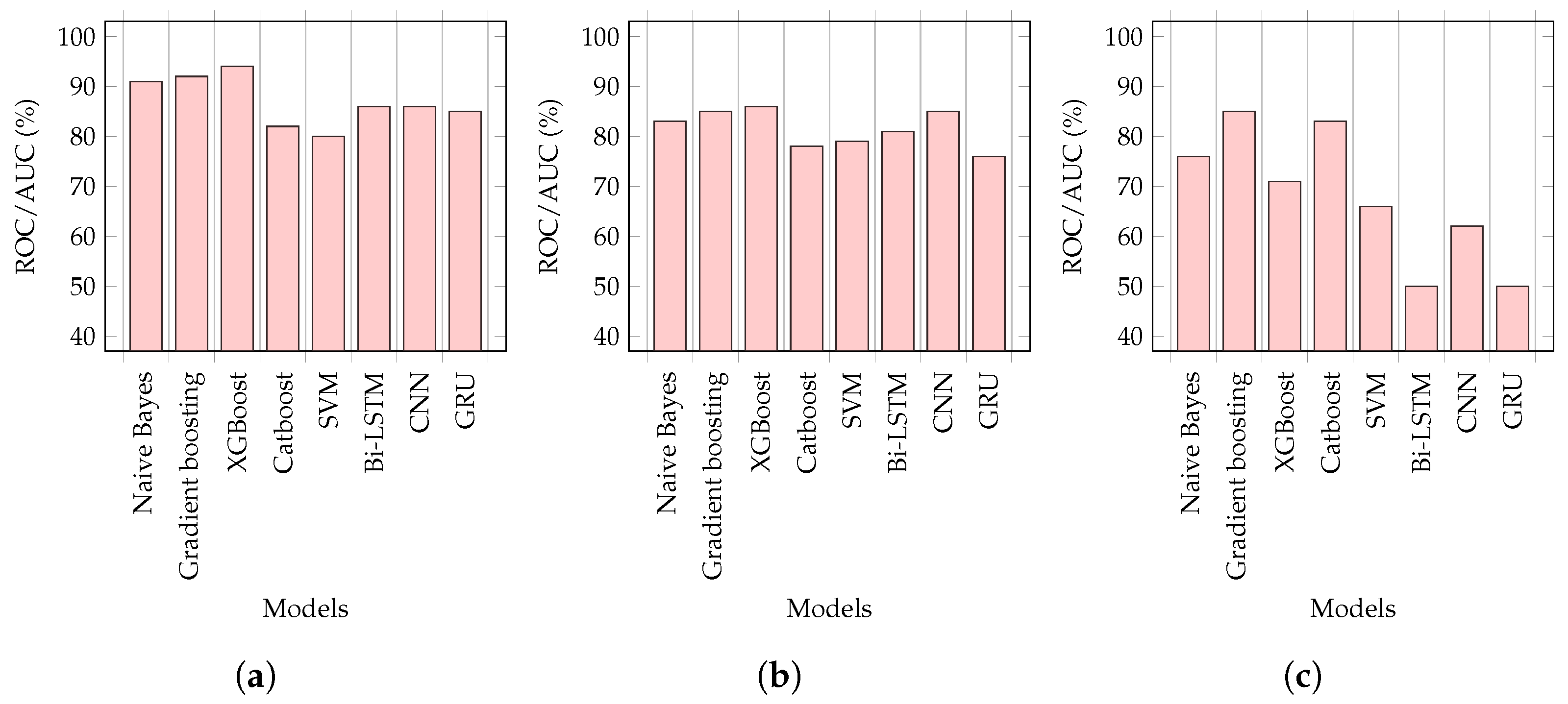
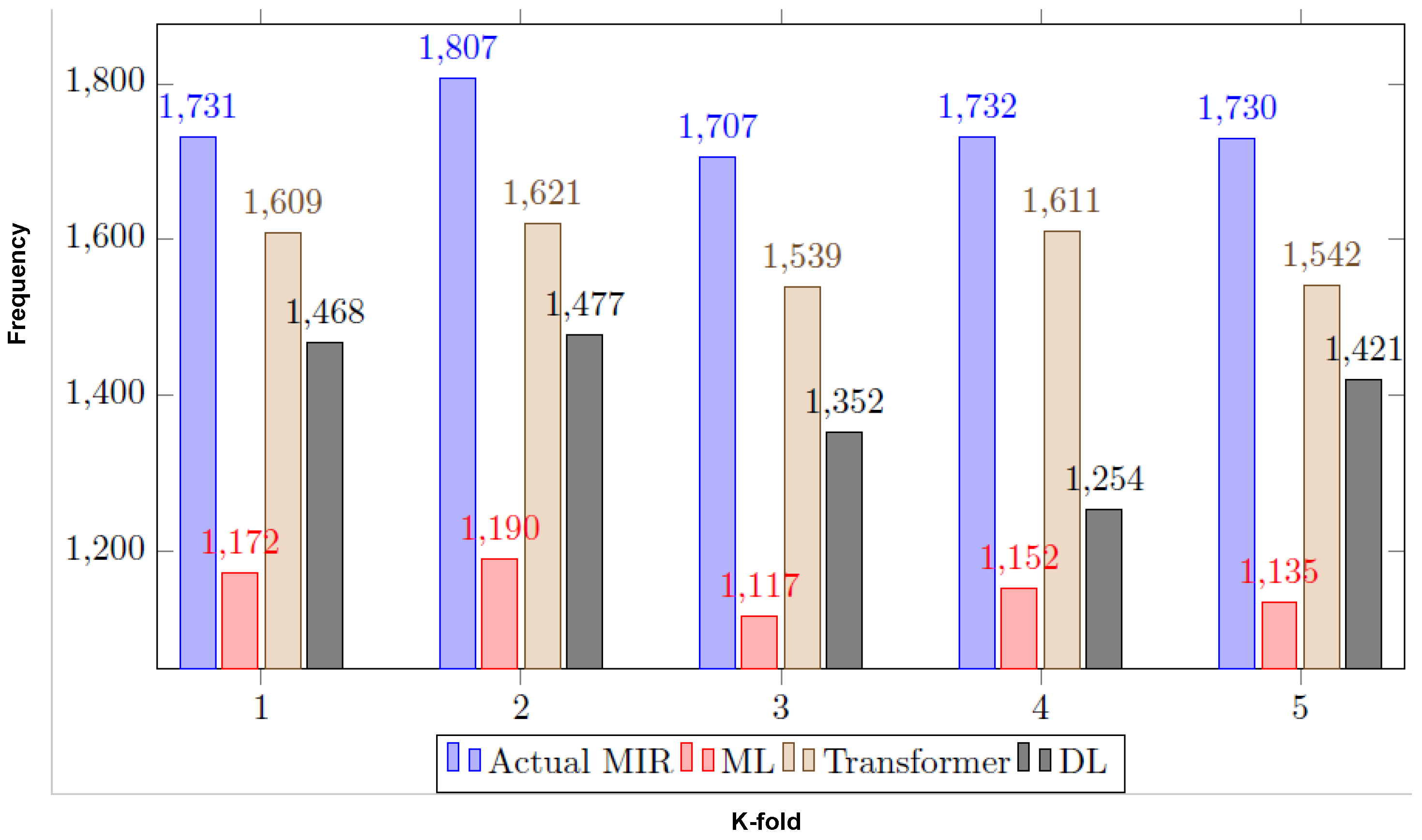
We found that accuracy was not the right performance metric because our initial results for imbalanced data were more skewed towards the majority class. We used a confusion matrix and area under the ROC curve to better quantify the correct and incorrect predictions. Based on our findings, the ROC metric showed the classifier’s exactness and completeness much better than accuracy. For example, Customer_records had the lowest minority class (MIR) records at 0.05%, which was highly imbalanced. Its ROC scores varied from 50% to 74%, whereas its accuracy score was 99%, which was misleading and highly skewed by the majority (NMIR) class. We calculated the confusion matrix by k-fold validation and the mean for each fold. Our results showed that RoBERTa possessed the highest mean score with 1462 TPs and 64,539 TNs values.

We calculated the prediction horizon to identify the average time for the ITSM system restoration from escalated deadlock. We targeted incident opened at(IOA) and MIR opened at(MOA) to calculate the prediction horizon. We evaluated the average incident escalation time, which was 2 h 30 min of saved time due to applying our proposed IT incident framework. It not only saved resources but also helped to prevent a deadlock situation. Considering the complexity of the prediction, the possibility of implementing RL to enhance these transformers is a significant possibility. At the time, we could identify any studies that were associated with RL implementation for IT incidents prediction. The convergence rate of RL models for classification was estimated to be 40% more, as compared to the other state-of-the-art model [56], which could hinder the adoption for large-scale industrial datasets. Furthermore, future work could involve evaluating NLPGym [57], a toolkit that bridges NLP and RL. The NLPGym provides a policy for reward and penalty against action, and deep-Q networks (DQN) could be used to train the model. We are optimistic that we can improve the accuracy score significantly through RL.

8. Conclusions

This paper leveraged state-of-art machine-learning (NB, SVM, GB, XGBoost, CatBoost), deep-learning (GRU, CNN, Bi-LSTM), and transformer architectures (BERT, Roberta, and ERNIE) to classify the provided incidents as major (MIR) and non-major (NMIR) to address the challenge of IT incident prediction. This paper was the first attempt to employ deep learning and transformers for solving IT service management problems, to the best of our knowledge. We experimented with three different sources of incidents: agency, customer, and employee. The transformer architectures (BERT, RoBERTa, and ERNIE) and XGBoost outperformed all other methods, with a 93% ROC for agency records, and with CNN, a 95% and 74% for employee and customers, respectively. To address the problem of data imbalance in our work, we resampled and curated synthetic data (SMOTE). With resampling, we achieved 95% with ERNIE for agency, 95% with BERT and ERNIE for employee, 99% with transformer and deep-learning models for customers, and 93% with BERT and ERNIE for all combined (employee, agency, and customer). For synthetic data, XGBoost had 94% for agency, 86% for employees, and with GB, 85% for customers. With the resampling and synthetic data curation, we noticed significant relative improvements, at 2.10% for agency and employees and 33% for the customer. We also identified the limitations of deep learning models for SMOTE, which we plan to address in the future. Additionally, our proposed framework computed the average prediction horizon, which was 2 h 30 min and leveraged this to minimize the meantime to resolve incidents. In the future, we will implement our framework for managing and reducing change failure rates associated with the incident mean time to resolution (MTTR). For future work, we are planning to perform a complete analysis of ITSM with state-of-the-art cross-validation techniques because the literature lacks this domain.

References

1. Cortina, S.; Barafort, B.; Picard, M.; Renault, A. Using a Process Assessment Model to Prepare for an ISO/IEC 20000-1 Certification: ISO/IEC 15504-8 or TIPA for ITIL? In Proceedings of the Systems, Software and Services Process Improvement—23rd European Conference, EuroSPI 2016, Graz, Austria, 14–16 September 2016; Communications in Computer and Information Science; Kreiner, C., O’Connor, R.V., Poth, A., Messnarz, R., Eds.; Springer: Berlin/Heidelberg, Germany, 2016; Volume 633, pp. 83–93. [Google Scholar] [CrossRef]
2. Lou, J.G.; Lin, Q.; Ding, R.; Fu, Q.; Zhang, D.; Xie, T. Software analytics for incident management of online services: An experience report. In Proceedings of the 2013 28th IEEE/ACM International Conference on Automated Software Engineering (ASE), Silicon Valley, CA, USA, 11–15 November 2013; pp. 475–485. [Google Scholar]
3. Bartolini, C.; Sallé, M.; Trastour, D. IT service management driven by business objectives An application to incident management. In Proceedings of the 2006 IEEE/IFIP Network Operations and Management Symposium NOMS 2006, Vancouver, BC, Canada, 3–7 April 2006; pp. 45–55. [Google Scholar]
4. Takeshita, K.; Yokota, M.; Nishimatsu, K. Early network failure detection system by analyzing Twitter data. In Proceedings of the 2015 IFIP/IEEE International Symposium on Integrated Network Management (IM), Ottawa, ON, Canada, 11–15 May 2015; pp. 279–286. [Google Scholar]
5. Zhou, W.; Tang, L.; Zeng, C.; Li, T.; Shwartz, L.; Grabarnik, G.Y. Resolution recommendation for event tickets in service management. IEEE Trans. Netw. Serv. Manag. 2016, 13, 954–967. [Google Scholar] [CrossRef]
6. Zhou, W.; Li, T.; Shwartz, L.; Grabarnik, G.Y. Recommending ticket resolution using feature adaptation. In Proceedings of the 2015 11th International Conference on Network and Service Management (CNSM), Barcelona, Spain, 9–13 November 2015; pp. 15–21. [Google Scholar]
7. Deljac, Ž.; Randić, M.; Krčelić, G. Early detection of network element outages based on customer trouble calls. Decis. Support Syst. 2015, 73, 57–73. [Google Scholar] [CrossRef]
8. Glenn, J.S.; Rose, K.L. Establishing Governance for Project and Service Management. In Proceedings of the 2019 ACM SIGUCCS Annual Conference, SIGUCCS 2019, New Orleans, LA, USA, 3–6 November 2019; Haring-Smith, B., McIntosh, K.M., Lineberry, B., Eds.; ACM: New York, NY, USA, 2019; pp. 145–147. [Google Scholar] [CrossRef] [Green Version]
9. Stoneburner, G.; Goguen, A.; Feringa, A. Risk Management Guide for Information Technology Systems; SP 800-30; National Institute of Standards and Technology: Gaithersburg, MD, USA, 2022. [Google Scholar]
10. Beresnev, A.; Gusarova, N. Comparison of Intelligent Classification Algorithms for Workplace Learning System in High-Tech Service-Oriented Companies. In Proceedings of the International Conference on Digital Transformation and Global Society, St. Petersburg, Russia, 17–19 June 2020; Springer: Berlin/Heidelberg, Germany, 2020; pp. 363–372. [Google Scholar]
11. Tolciu, D.T.; Sacarea, C.; Matei, C. Analysis of Patterns and Similarities in Service Tickets using Natural Language Processing. J. Commun. Softw. Syst. 2021, 17, 29–35. [Google Scholar] [CrossRef]
12. Nikulin, V.; Shibaikin, S.; Vishnyakov, A. Application of machine learning methods for automated classification and routing in ITIL. J. Phys. Conf. Ser. 2021, 2091, 012041. [Google Scholar] [CrossRef]
13. Kodepogu, K.R.; Annam, J.R.; Vipparla, A.; Krishna, B.V.N.V.S.; Kumar, N.; Viswanathan, R.; Gaddala, L.K.; Chandanapalli, S.K. A Novel Deep Convolutional Neural Network for Diagnosis of Skin Disease. Trait. Signal 2022, 39, 1873–1877. [Google Scholar] [CrossRef]
14. Devlin, J.; Chang, M.W.; Lee, K.; Toutanova, K. Bert: Pre-training of deep bidirectional transformers for language understanding. arXiv 2018, arXiv:1810.04805. [Google Scholar]
15. Liu, Y.; Ott, M.; Goyal, N.; Du, J.; Joshi, M.; Chen, D.; Levy, O.; Lewis, M.; Zettlemoyer, L.; Stoyanov, V. RoBERTa: A Robustly Optimized BERT Pretraining Approach. arXiv 2019, arXiv:1907.11692. [Google Scholar]
16. Sun, Y.; Wang, S.; Li, Y.; Feng, S.; Tian, H.; Wu, H.; Wang, H. ERNIE 2.0: A continual pre-training framework for language understanding. In Proceedings of the AAAI Conference on Artificial Intelligence, New York, NY, USA, 7–12 February 2020; Volume 34, pp. 8968–8975. [Google Scholar]
17. Ali Zaidi, S.S.; Fraz, M.M.; Shahzad, M.; Khan, S. A multiapproach generalized framework for automated solution suggestion of support tickets. Int. J. Intell. Syst. 2022, 37, 3654–3681. [Google Scholar] [CrossRef]
18. Gouryraj, S.; Kataria, S.; Swvigaradoss, J. Service Level Agreement Breach Prediction in ServiceNow. In Proceedings of the 2021 Third International Conference on Inventive Research in Computing Applications (ICIRCA), Coimbatore, India, 2–4 September 2021; pp. 689–698. [Google Scholar]
19. Agarwal, S.; Aggarwal, V.; Akula, A.R.; Dasgupta, G.B.; Sridhara, G. Automatic problem extraction and analysis from unstructured text in IT tickets. IBM J. Res. Dev. 2017, 61, 4–41. [Google Scholar] [CrossRef]
20. Pedregosa, F.; Varoquaux, G.; Gramfort, A.; Michel, V.; Thirion, B.; Grisel, O.; Blondel, M.; Prettenhofer, P.; Weiss, R.; Dubourg, V.; et al. Scikit-learn: Machine Learning in Python. J. Mach. Learn. Res. 2011, 12, 2825–2830. [Google Scholar]
21. Zhao, H.; Lai, Z.; Leung, H.; Zhang, X. A Gentle Introduction to Feature Learning. In Feature Learning and Understanding; Springer: Berlin/Heidelberg, Germany, 2020; pp. 1–12. [Google Scholar]
22. Al Qadi, L.; El Rifai, H.; Obaid, S.; Elnagar, A. A scalable shallow learning approach for tagging arabic news articles. Jordanian J. Comput. Inf. Technol. 2020, 6, 263–280. [Google Scholar]
23. Ye, Y.; Ma, F.; Lu, Y.; Chiu, M.; Huang, J.Z. iSurfer: A Focused Web Crawler Based on Incremental Learning from Positive Samples. In Proceedings of the Advanced Web Technologies and Applications, 6th Asia-Pacific Web Conference, APWeb 2004, Hangzhou, China, 14–17 April 2004; Lecture Notes in Computer Science; Yu, J.X., Lin, X., Lu, H., Zhang, Y., Eds.; Springer: Berlin/Heidelberg, Germany, 2004; Volume 3007, pp. 122–134. [Google Scholar] [CrossRef]
24. Revina, A.; Buza, K.; Meister, V.G. IT Ticket Classification: The Simpler, the Better. IEEE Access 2020, 8, 193380–193395. [Google Scholar] [CrossRef]
25. Revina, A.; Buza, K.; Meister, V.G. Designing Explainable Text Classification Pipelines: Insights from IT Ticket Complexity Prediction Case Study. Interpret. Artif. Intell. A Perspect. Granul. Comput. 2021, 937, 293. [Google Scholar]
26. Zuev, D.; Kalistratov, A.; Zuev, A. Machine learning in IT service management. Procedia Comput. Sci. 2018, 145, 675–679. [Google Scholar] [CrossRef]
27. Costa, J.; Pereira, R.; Ribeiro, R. ITSM automation-Using machine learning to predict incident resolution category. In Proceedings of the 33rd International Business Information Management Association Conference: Education Excellence and Innovation Management through Vision 2020, IBIMA 2019, Granada, Spain, 10–11 April 2019; pp. 5819–5830. [Google Scholar]
28. Wang, Q.; Zeng, C.; Iyengar, S.; Li, T.; Shwartz, L.; Grabarnik, G.Y. AISTAR: An intelligent system for online IT ticket automation recommendation. In Proceedings of the 2018 IEEE International Conference on Big Data (Big Data), Seattle, WA, USA, 10–13 December 2018; pp. 1875–1884. [Google Scholar]
29. Al-Hawari, F.; Barham, H. A machine learning based help desk system for IT service management. J. King Saud Univ. Comput. Inf. Sci. 2021, 33, 702–718. [Google Scholar] [CrossRef]
30. Paramesh, S.; Shreedhara, K. IT Help Desk Incident Classification using Classifier Ensembles. ICTACT J. Soft Comput. 2019, 9, 1980–1987. [Google Scholar]
31. Gupta, R.; Prasad, K.H.; Mohania, M. Automating ITSM incident management process. In Proceedings of the 2008 International Conference on Autonomic Computing, Chicago, IL, USA, 2–6 June 2008; pp. 141–150. [Google Scholar]
32. Altintas, M.; Tantug, A.C. Machine learning based ticket classification in issue tracking systems. In Proceedings of the International Conference on Artificial Intelligence and Computer Science (AICS 2014), Bandung, Indonesia, 15–16 September 2014; pp. 195–207. [Google Scholar]
33. Silva, S.; Pereira, R.; Ribeiro, R. Machine learning in incident categorization automation. In Proceedings of the 2018 13th Iberian Conference on Information Systems and Technologies (CISTI), Caceres, Spain, 13–16 June 2018; pp. 1–6. [Google Scholar]
34. Paramesh, S.; Shreedhara, K. Automated IT service desk systems using machine learning techniques. In Data Analytics and Learning; Springer: Berlin/Heidelberg, Germany, 2019; pp. 331–346. [Google Scholar]
35. Roy, S.; Muni, D.P.; Tack Yan, J.J.Y.; Budhiraja, N.; Ceiler, F. Clustering and labeling IT maintenance tickets. In Proceedings of the International Conference on Service-Oriented Computing, Banff, AB, Canada, 10–13 October 2016; pp. 829–845. [Google Scholar]
36. Schad, J.; Sambasivan, R.; Woodward, C. Predicting help desk ticket reassignments with graph convolutional networks. Mach. Learn. Appl. 2022, 7, 100237. [Google Scholar] [CrossRef]
37. Aglibar, K.D.; Alegre, G.C.; Del Mundo, G.; Duro, K.F.; Rodelas, N. Ticketing System: A Descriptive Research on the Use of Ticketing System for Project Management and Issue Tracking in IT Companies. arXiv 2022, arXiv:2202.06213. [Google Scholar]
38. YAYAH, F.C.; Ghauth, K.I.; TING, C.Y. The automated machine learning classification approach on telco trouble ticket dataset. J. Eng. Sci. Technol. 2021, 16, 4263–4282. [Google Scholar]
39. Bajpai, H. Building ML Based Intelligent System to Analyze Production LSI (Live Site Incidents). Int. J. Eng. Adv. Technol. (IJEAT) 2021, 10, 41–46. [Google Scholar] [CrossRef]
40. Shorten, C.; Khoshgoftaar, T.M.; Furht, B. Text Data Augmentation for Deep Learning. J. Big Data 2021, 8, 101. [Google Scholar] [CrossRef] [PubMed]
41. Chawla, N.V.; Bowyer, K.W.; Hall, L.O.; Kegelmeyer, W.P. SMOTE: Synthetic minority over-sampling technique. J. Artif. Intell. Res. 2002, 16, 321–357. [Google Scholar] [CrossRef]
42. Webb, G.I.; Keogh, E.; Miikkulainen, R. Naïve Bayes. Encycl. Mach. Learn. 2010, 15, 713–714. [Google Scholar]
43. Mayr, A.; Binder, H.; Gefeller, O.; Schmid, M. The evolution of boosting algorithms. Methods Inf. Med. 2014, 53, 419–427. [Google Scholar] [PubMed] [Green Version]
44. Chen, T.; He, T.; Benesty, M.; Khotilovich, V.; Tang, Y.; Cho, H.; Chen, K.; Mitchell, R.; Cano, I.; Zhou, T. Xgboost: Extreme Gradient Boosting; R Package; R Code Team: Vienna, Austria, 2015; pp. 1–4. [Google Scholar]
45. Couronné, R.; Probst, P.; Boulesteix, A.L. Random forest versus logistic regression: A large-scale benchmark experiment. BMC Bioinform. 2018, 19, 270. [Google Scholar] [CrossRef] [Green Version]
46. Dorogush, A.V.; Ershov, V.; Gulin, A. CatBoost: Gradient boosting with categorical features support. arXiv 2018, arXiv:1810.11363. [Google Scholar]
47. Ke, G.; Meng, Q.; Finley, T.; Wang, T.; Chen, W.; Ma, W.; Ye, Q.; Liu, T.Y. Lightgbm: A highly efficient gradient boosting decision tree. Adv. Neural Inf. Process. Syst. 2017, 30, 1–9. [Google Scholar]
48. Suthaharan, S. Support vector machine. In Machine Learning Models and Algorithms for Big Data Classification; Springer: Berlin/Heidelberg, Germany, 2016; pp. 207–235. [Google Scholar]
49. Schuster, M.; Paliwal, K.K. Bidirectional recurrent neural networks. IEEE Trans. Signal Process. 1997, 45, 2673–2681. [Google Scholar] [CrossRef] [Green Version]
50. O’Shea, K.; Nash, R. An Introduction to Convolutional Neural Networks. arXiv 2015, arXiv:1511.08458. [Google Scholar]
51. Collobert, R.; Weston, J. A unified architecture for natural language processing: Deep neural networks with multitask learning. In Proceedings of the 25th International Conference on Machine Learning, Helsinki, Finland, 5–9 July 2008; pp. 160–167. [Google Scholar]
52. Cho, K.; Van Merriënboer, B.; Bahdanau, D.; Bengio, Y. On the properties of neural machine translation: Encoder-decoder approaches. arXiv 2014, arXiv:1409.1259. [Google Scholar]
53. Bird, S.; Loper, E. NLTK: The Natural Language Toolkit. In Proceedings of the ACL Interactive Poster and Demonstration Sessions; Association for Computational Linguistics: Barcelona, Spain, 2004; pp. 214–217. [Google Scholar]
54. Ling, C.X.; Huang, J.; Zhang, H. AUC: A Better Measure than Accuracy in Comparing Learning Algorithms. In Advances in Artificial Intelligence; Xiang, Y., Chaib-draa, B., Eds.; Springer: Berlin/Heidelberg, Germany, 2003; pp. 329–341. [Google Scholar]
55. Prokhorenkova, L.; Gusev, G.; Vorobev, A.; Dorogush, A.V.; Gulin, A. CatBoost: Unbiased boosting with categorical features. Adv. Neural Inf. Process. Syst. 2018, 31, 1–11. [Google Scholar]
56. Lagoudakis, M.G.; Parr, R. Reinforcement learning as classification: Leveraging modern classifiers. In Proceedings of the 20th International Conference on Machine Learning (ICML-03), Washington, DC, USA, 21–24 August 2003; pp. 424–431. [Google Scholar]
57. Ramamurthy, R.; Sifa, R.; Bauckhage, C. NLPGym—A toolkit for evaluating RL agents on Natural Language Processing Tasks. 2020. Available online: http://xxx.lanl.gov/abs/2011.08272 (accessed on 30 August 2022).
Figure 1. Overview of IT incident management system.
Applsci 13 03843 g001
Figure 2. Distribution of dataset.
Applsci 13 03843 g002
Figure 3. Proposed IT incident risk framework.
Applsci 13 03843 g003
Figure 4. Graphical representation of the pipeline stages for training and testing for ML, DL, and transformer models.
Applsci 13 03843 g004
Figure 5. Graphical representation of our best-performing transformer (Roberta) model architecture.
Applsci 13 03843 g005
Figure 6. Average tokenizer/class for training and test data across (a) Agency_records, (b) Employee_records and (c) Customer_records.
Applsci 13 03843 g006
Figure 7. Quantitative ROC/AUC results across (a) Agency_records, (b) Employee_records, and (c) Customer_records for state-of-art methods.
Applsci 13 03843 g007
Figure 8. Quantitative ROC/AUC results across (a) Agency_resampled, (b) Employee_resampled (c) Customer_resampled, and (d) Combine_All for state-of-art methods.
Applsci 13 03843 g008
Figure 9. Qualitative ROC/AUC results for synthetic data (SMOTE) across (a) agency, (b) employee and (c) customer for state-of-art methods.
Applsci 13 03843 g009
Figure 10. ROC/AUC results across k-fold cross-validation.
Applsci 13 03843 g010
Figure 11. Number of MIR across actual, ML (naive Bayes, gradient boost, XGBoost, CatBoost, SVM), transformers (BERT, RoBERTa, ERNIE 2.0), and DL algorithms(GRU, Bi-LSTM, CNN).
Applsci 13 03843 g011
Figure 12. Prediction horizon comparison (MIR opened at vs. incident opened at. The blue line indicates IOA records while the orange shows the MOA records).
Applsci 13 03843 g012
Figure 13. Prediction horizon comparison (MIR opened at vs. incident opened at).
Applsci 13 03843 g013