1. Introduction
The crewed lunar roving vehicle (CLRV) is essential in Chinese plans to build a lunar base. The CLRV is an essential and indispensable exploration tool that not only transports astronauts to great distances from the lunar module but also ensures their safety as they move on the lunar surface [
1]. To mitigate the potential issues of the CLRV, it is imperative to conduct a comprehensive ground test of the full rover before launch. Furthermore, the differences in gravity between the Moon and Earth give rise to distinct steering properties and driving sensations for the astronauts using the CLRV. Therefore, it is essential to construct a ground test facility on Earth that accurately simulates lunar gravity to facilitate astronaut training and evaluate the CLRV’s performance.
A problem common to the ground test facility is simulating a low-gravity environment similar to the spacecraft’s natural working environment [
2]. Simulating a low-gravity field is an essential issue in the motion performance experiment of the planetary rover. The simulation method of offsetting part of the lunar rover’s gravity by an external force is called gravity compensation. The primary ways to achieve artificial micro-gravity include free-fall testing [
3], the air-bearing table [
4], neutral buoyance [
5,
6], and the suspension system [
7,
8]. Among the available methods, the suspension system [
9,
10] is widely adopted because of its relatively simple structure, easy construction, and 3-D simulation with unlimited time.
The track-following servo subsystem is a critical component of the suspension gravity compensation system, which is used to precisely track the movement of the test object in the horizontal direction. In the suspension gravity compensation system of the CLRV, due to the large motion velocity, acceleration, and range of the CLRV, the track-following servo subsystem also requires a corresponding motion capability and a large scale. In this context, the crane as the servo motion mechanism exhibits significant inertial characteristics [
11]. At the same time, the subsystem is also faced with various constraints such as speed, acceleration, and position. These characteristics often result in significant tracking errors and even control failure.
Currently, research on the effectiveness of the track-following servo subsystem in the suspension gravity compensation system of the CLRV remains unexplored. The active response gravity offload system (ARGOS) at NASA’s Johnson Space Center is a typical suspension system [
12]. However, the track-following servo subsystem of this system is only applicable for walking tests of astronauts with low velocity in a single direction. The Harbin Institute of Technology built a suspension lunar gravity compensation system, which was only suitable for slow-moving unmanned lunar rovers [
2]. The max speed of the Yutu lunar rover is about 200 m/h, while the theoretical maximum speed of the CLRV in pre-research is about 4 m/s. The Soviet Union’s planetary rover ground test used an active tracking constant tension suspension scheme [
13], which generated a constant vertical pulling force using a parallelogram with a spring. However, this solution is only suitable for ground tests on Mars rovers and may not work well for driving a large vehicle on simulated soft lunar soil. NASA proposed a suspension system scheme suitable for CLRV ground tests in the last century, but the track-following servo control in the program lacks simulation validation and practical implementation [
14]. The suspended gravity compensation system is more commonly used in slow-motion microgravity experiments, such as deployable antennas [
7] and satellites [
8], and its tracking servo subsystem is not suitable for the CLRV.
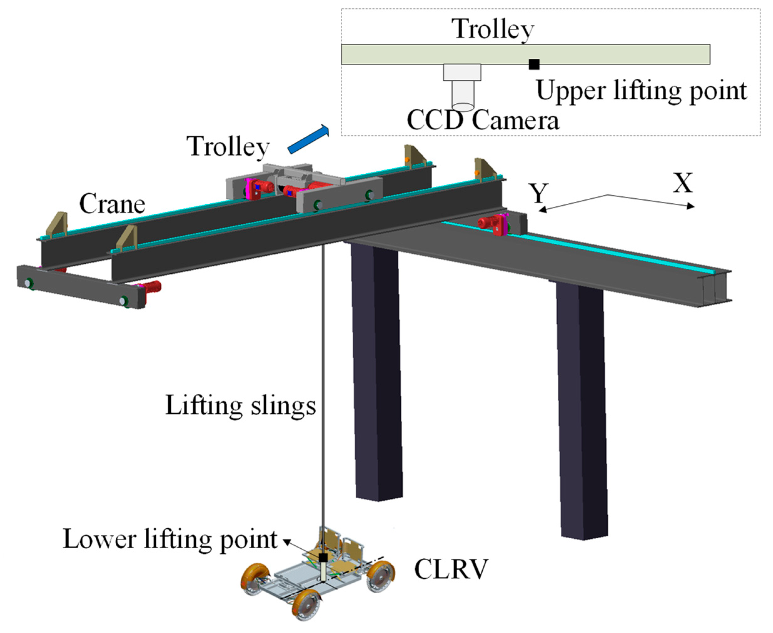
To meet the CLRV’s test requirements, this paper conducts research on the system design and control scheme of the track-following servo subsystem in an overhead-crane-like Lunar Gravity Compensation facility (LGCF) based on a single-cable gravity compensation system. As shown in
Figure 1, the system compensates 5/6 of the CLRV’s weight over a square test field of 80 × 20 square meters. As shown in
Figure 1, the primary research of this paper is the track-following servo subsystem in the LGCF, consisting of an overhead moving crane and a trolley. The crane moves on the bridge, tracking the real-time position of the CLRV in the
direction, and the trolley moves along the crane girder to follow the real-time
position of the CLRV. The servo motors drive the crane and trolley.
The paper introduces the vector control of the PMSM to the track-following servo subsystem, enabling high-precision and rapid tracking control. In servo motors, the permanent-magnet synchronous motor (PMSM) has many outstanding advantages compared with other motors. The PMSM vector control system can achieve high precision, high dynamic performance, and an extensive range of speed regulation, tracking, and control, attracting wide attention and research from scholars worldwide [
15,
16,
17].
This track-following servo subsystem includes the position servo closed-loop and closed-loop control of the motor speed and current. In the simulation model of the speed and current closed-loop control, the surface-mounted PMSM (SPMSM) vector control system based on the Space Vector Pulse Width Modulation (SVPWM) method was used in the paper [
18], which highly simulated the actual system. The PI method was used for the PMSM vector control system.
In the position servo closed-loop, there are constraints on the movement speed and acceleration of the crane and trolley to avoid motor idling [
19] or over-speed. Moreover, the motion ranges of the crane and trolley are also constrained by the size of the facility. The traditional PID control cannot meet the control requirements, due to multi-variable constraints in the position servo closed-loop. In particular, this paper employs the explicit model predictive controller (EMPC) [
20] in the position servo closed-loop so that the overhead moving crane and the trolley follow the motion of the CLRV in the
and
directions, respectively. The MPC is a new computer optimization control algorithm that can effectively deal with multi-variable constraint systems [
21]. It has become a standard optimization method for complex constraint systems. In recent years, the MPC has received significant attention in path tracking and fast tracking [
22,
23]. The main reason is that the MPC can better handle the constraints of concern to physical and safety systems, which benefits system control performance and component protection. Despite the advantages of the MPC mentioned above, its substantial computational complexity resulting from online optimization at each sampling time poses a significant drawback and limits its applicability to relatively small and slow systems. To address this challenge, Bemporad and Alberto et al. proposed a novel approach based on an MPC scheme that moves all computational efforts offline, enabling the scheme to overcome the aforementioned limitation [
24,
25], and the method is the EMPC.
Overall, this study provides an innovative and promising design proposal for a track-following servo subsystem of an LGCS suitable for the CLRV ground test. The vector control of the PMSM based on SVPWM is used in this paper to achieve a fast response of the track-following servo control. Notably, this paper adopts an EMPC in the position servo closed-loop to obtain good control performance. The EMPC controller can be applied to multi-constrained systems, ensuring a fast response while reducing overshoot. Finally, simulation models of the subsystem are built, and the simulation results are presented and discussed to evaluate the proposed system design and control scheme. The study provides a significant contribution to the field of the LGCS and serves as a valuable reference for future research.
The paper is organized as follows.
Section 2 presents the design scheme of the tracking servo subsystem and establishes the system’s three-loop servo control model of the current loop, speed loop, and position loop.
Section 3 introduces the implementation process of the EMPC control strategy. In
Section 4, the desired trajectory of the system, EMPC, and LQI position loop control model parameters are presented.
Section 5 discusses and presents the simulation results to evaluate the system performance. Finally,
Section 6 concludes the paper.
2. Methodology
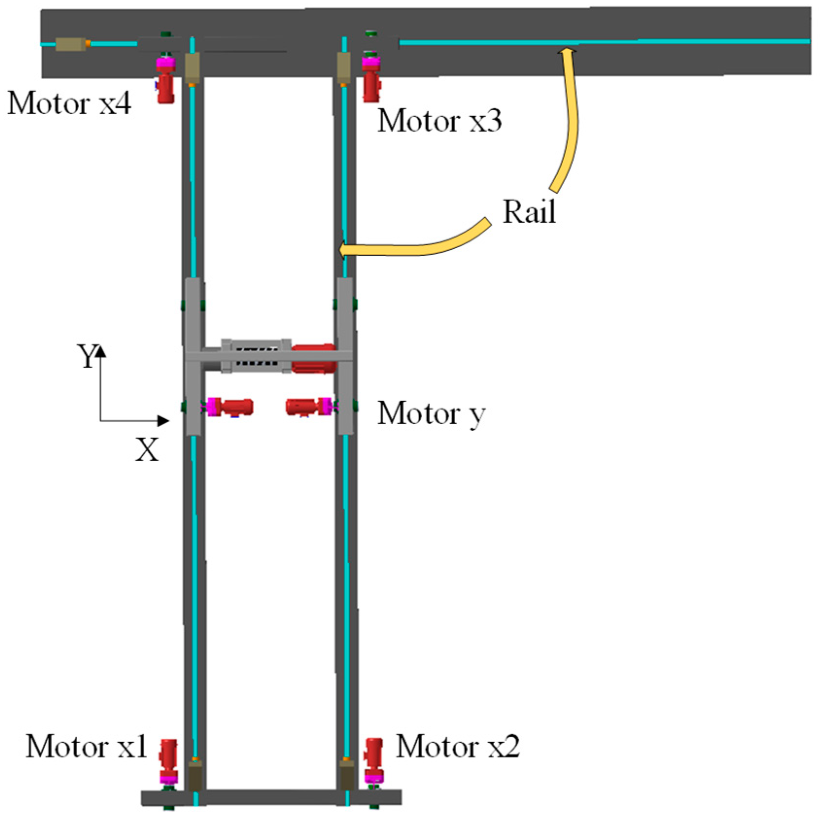
In this section, we present the mechanical design of the track-following servo subsystem. The subsystem comprises a moving crane system, a moving trolley system, and multiple motors that enable the track-following servo in both the
X and
Y directions, as illustrated in
Figure 2. The crane is driven by four motors, and the trolley is driven by two motors. The motors power the steel wheels of the crane and trolley to move on the rail. The servo motors transmit power to the system, which is then transmitted to the low-speed shaft end of the reducer via the coupling. The reducer’s low-speed shaft end outputs to the driving wheel shaft through another coupling, and the driving wheels propel the crane and trolley to follow the CLRV with high precision.
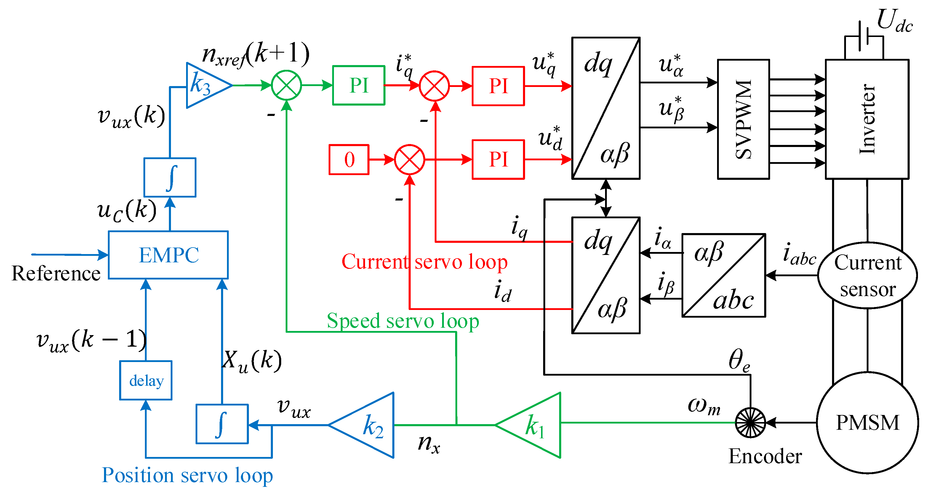
Then, based on the mechanical design of the subsystem, suitable equipment is selected, and a simulation model of the track-following servo subsystem is established. In this paper, the servo motors used are PMSMs. The track-following servo subsystem comprises a position servo closed-loop and closed-loop control of the motor speed and current; the crane control model is illustrated in
Figure 3. The position control loop is situated on the outer layer of the double closed-loop, which includes the speed and current loops of the servo motor. The position control loop receives a reference signal and subsystem state variables and calculates the expected velocity increment of the crane or trolley in a given unit of time. This value is then passed to the motor’s speed loop controller. The speed loop controller calculates the expected current output by comparing the expected speed with the actual speed. The motor’s current loop controller then calculates the expected voltage input based on the expected current and the actual current. Together, these three loops form the track-following servo subsystem.
To achieve high-precision control of the crane and trolley, the PMSM vector control method based on SVPWM is adopted for fast response in speed control. The PI control method, with its advantages of being a simple algorithm, having good stability, and having high reliability in the motor speed control system, is widely used for controlling motor speed and current. Therefore, the PI method is applied to the PMSM vector control system, as depicted in
Figure 3.
The performance of the outermost position servo loop plays a crucial role in the track-following servo subsystem’s tracking performance. However, the position loop’s control is limited by the electromechanical system’s kinematics and dynamics. To overcome this multi-parameter constraint, the present paper proposes utilizing the EMPC controller within the position servo closed-loop.
This section mainly describes the establishment of the mathematical model for the three-loop control system, including the mathematical model and model parameters of the PMSM, as well as the mathematical model of the position loop.
2.1. Mathematical Model of PMSM
As shown in
Figure 3, this paper adopts vector control technology based on SVPWM to realize the decoupling control of torque and excitation components. Following the stator flux linkage orientation control rules, the d-axis of the reference coordinate is aligned with the motor flux direction, where
. The stator flux linkage component on the d-axis is represented as
. The voltage equation of the PMSM is formulated in the two-phase synchronous rotating reference frame.
The torque reference (electromagnetic torque)
in the following equation is used:
where
is the stator resistance (
);
and
are the inductances (
) of the stator on the
and
axes, respectively;
and
are the current (
) of the stator on the
and
axes, respectively;
and
are the voltage (
) of the stator on the
and
axes, respectively;
is the number of pole pairs of the rotor;
is the inertia;
is the angular velocity measured from the motor;
is a constant load torque;
is the mechanical damping constant.
Suppose that the load torque of the four motors in the direction is equal, the output torque and speed are equal, the load torque of the two motors in the direction is equal, and the output torque and speed are equal. In order to build the mathematical model of the motor, it is necessary to select the specific motor first according to the required motor torque and speed.
The motor torque
is divided into load torque
for overcoming rolling friction and accelerating torque
for maximum acceleration.
where the gross load hauled by the crane is about
= 12,000 kg, and the gross load hauled by the trolley is about
. The number of motors for the moving crane system and the moving trolley system are
and
, respectively. The coefficient of rolling friction with railroad steel wheels on steel rails is
, and the radius of the steel wheel is
.
The design speed of the crane is larger than the maximum speed () of the CLRV, so m/s is set. Additionally, the VLRV moves in a small range in the Y direction, so m/s is set. The and are the actual speeds of the crane and trolley, respectively.
According to Equation (4), the max speeds of motors
and
can be calculated:
where the gear ratio of the crane motors is
and the gear ratio of the trolley motors is
.
According to the calculation, the motors are selected. The parameters of the motors are shown in the following
Table 1.
In the system, the motors’ speeds are
and
, and the actual angular velocities of the motors are
and
, respectively.
In this paper, the PI control is adopted in the motor’s current loop and speed loop control. The primary constraints during the controller design are the voltage and current constraints on the quadrature axis and direct axis. The constraints are as follows:
As this is a real physical system, constraints on the states and inputs have to be considered during the controller design given. In the wheel/rail transmission, the premise for obtaining different traction forces is not to destroy the adhesion moment between the wheel/rail. In this paper, the calculation formula of the train wheel/rail adhesion coefficient
is used to calculate the maximum traction torque. When the train speed
km/h, the
is as follows [
26]:
Then, the maximum traction torque is
The maximum accelerations
and
can be calculated from the maximum output torque
:
The maximum accelerations of the crane and trolley are and , respectively.
Additionally, this system adopts 17-bit incremental rotary encoders to measure the angular velocity and rotor-position of the motors. The measurement error of the motor rotor-position is 0.001°, and the measurement error of the motor angular velocity is 0.2 rad/s. Rotor-position measurement noise adds Gaussian white noise to the , the amplitude is 0.001°, and the sampling period is 1/10,000 s. Angular velocity measurement noise adds Gaussian white noise to the angular velocity feedback , the amplitude is 0.2 rad/s, and the sampling period is 1/10,000 s. The current measurement noise also adds Gaussian white noise to the feedback loop of and , the noise amplitude is 0.2 A, and the sampling period is 1/10,000 s. The discrete signals , , and are delayed by one sampling period. Then, the signals are passed to the PI controllers or converters.
2.2. Position Servo Loop Model
In this paper, the position servo loop receives the lifting points’ information from the position and orientation measurement system. The EMPC controller outputs the desired movement increment of the crane in the direction and the desired movement increment of the trolley in the direction. In this section, the subscript C denotes the crane and the subscript T denotes the trolley.
Under the fixed coordinates
on the ground, the kinematic equation of the trolley and crane in
and
directions is as follows:
where
and
are the position of the crane and trolley in the coordinate system
,
In
Figure 3,
(rpm) is the reference speed of the motor that drives the crane to move in the
direction, and
(rpm) is the reference speed of the motor that drives the trolley to move in the
direction. The relationship between
and
is as follows:
When designing the position loop servo controller, the position servos of the
and
directions are designed independently. In engineering, the system control generally adopts the incremental control method, and the incremental control is to output the increment
of the control variable
every period:
The reference signal can be regarded as a state variable:
The state-space models for the moving crane system and the moving trolley system are as follows:
where
The deviation in the crane and trolley’s position in the X and Y directions from the desired trajectory converges to zero through the proposed control scheme. To implement Equations (17) and (18) in an explicit MPC scheme, a zero-order hold method with a sampling time of 0.005 s is utilized in this paper.
3. Explicit Model Predictive Control
To ensure robustness and meet complex constraints, this study employs MPC [
27,
28] as a crucial optimal control scheme. At each sampling time k, the optimal control law of the inner loop is solved by formulating and solving a control problem that is then transformed into an online quadratic programming (QP) problem. The cost function used in this control problem is defined as follows:
where
,
, and
are the discrete-time versions of the system, input, and output matrices, respectively.
is the prediction horizon and
is the control horizon. The notation
represents the predicted value of
at
steps ahead of
. Here,
,
, and
are the weighting matrices for the state, input, and terminal state, respectively.
is the output weighting matrix used to measure tracking error.
In addition, the output can be obtained with corresponding dimensions
and
by solving the discrete-time algebraic Riccati equation [
29], given by
Using these weighting matrices, the MPC controller computes a sequence of optimal vectors that minimize the cost function .
Although MPC offers several advantages, such as optimal control and handling of constraints, the online optimization process can lead to a significant computational burden, which is a major drawback. To address this issue, Alberto proposed a new MPC scheme that can reduce the computational load [
30].
The equations for predicting the state vector
can be obtained through the following derivation:
where
Equations (19) and (21) can be reformulated as follows:
where
By defining
,
, and
, Equation (22) can be formulated as the following equivalent form:
where
In Equation (23), indicates the th row of .
By defining
, the reformulated optimization problem presented in Equation (23) can be expressed as a mixed-integer quadratic programming (mp-QP) problem, as shown below [
24]:
where
and
.
The Karush–Kuhn–Tucker (KKT) optimization conditions are used for the above problem [
30]:
Solving the above equations:
Based on the above equation, it can be observed that Equations (26) and (27) are linear affine functions of the state . Furthermore, it is apparent that the control variable is also a linear affine function of the state when considered in conjunction with equation . The subscript indicates the active constraint, and the subscript indicates the inactive constraint.
Based on the KKT condition, it is evident that the validity of the above equation is contingent on satisfying the inequality constraints:
The polyhedral set (critical region)
can be formed:
By applying different constraints, more critical regions are formed for different groups of states. Therefore, a map of states to optimal control inputs is eventually created.
5. Results and Discussion
In this system, the impact of the tracking error of the track-following system mainly includes the impact on the drawbar pull force
[
33] and gravity compensation force
of the CLRV.
Supposing that the upper lifting point is positioned 10 m above the CLRV, the drawbar pull force error in the horizontal direction caused by the tracking error denoted as
can be expressed as:
where
is the weight of the CLRV and
is the tracking error.
The gravity compensation force error
in the vertical direction caused by the position tracking error is:
Supposing that the drawbar pull factor of the CLRV’s wheel with a radius of 0.4 m on loose soil is
, the maximum drawbar pull force and gravity compensation force can be roughly expressed as:
where
is the wheel vertical load. Hence, the maximum drawbar pull of the entire rover can be estimated by setting
as 1/6
.
Combining Equations (35)–(38) gives:
where
and
are the error impact factors to measure the influence of tracking errors.
This section presents and discusses the simulation results of the track-following servo control for paths one, two, three, and four using the PI, LQI, and EMPC controllers.
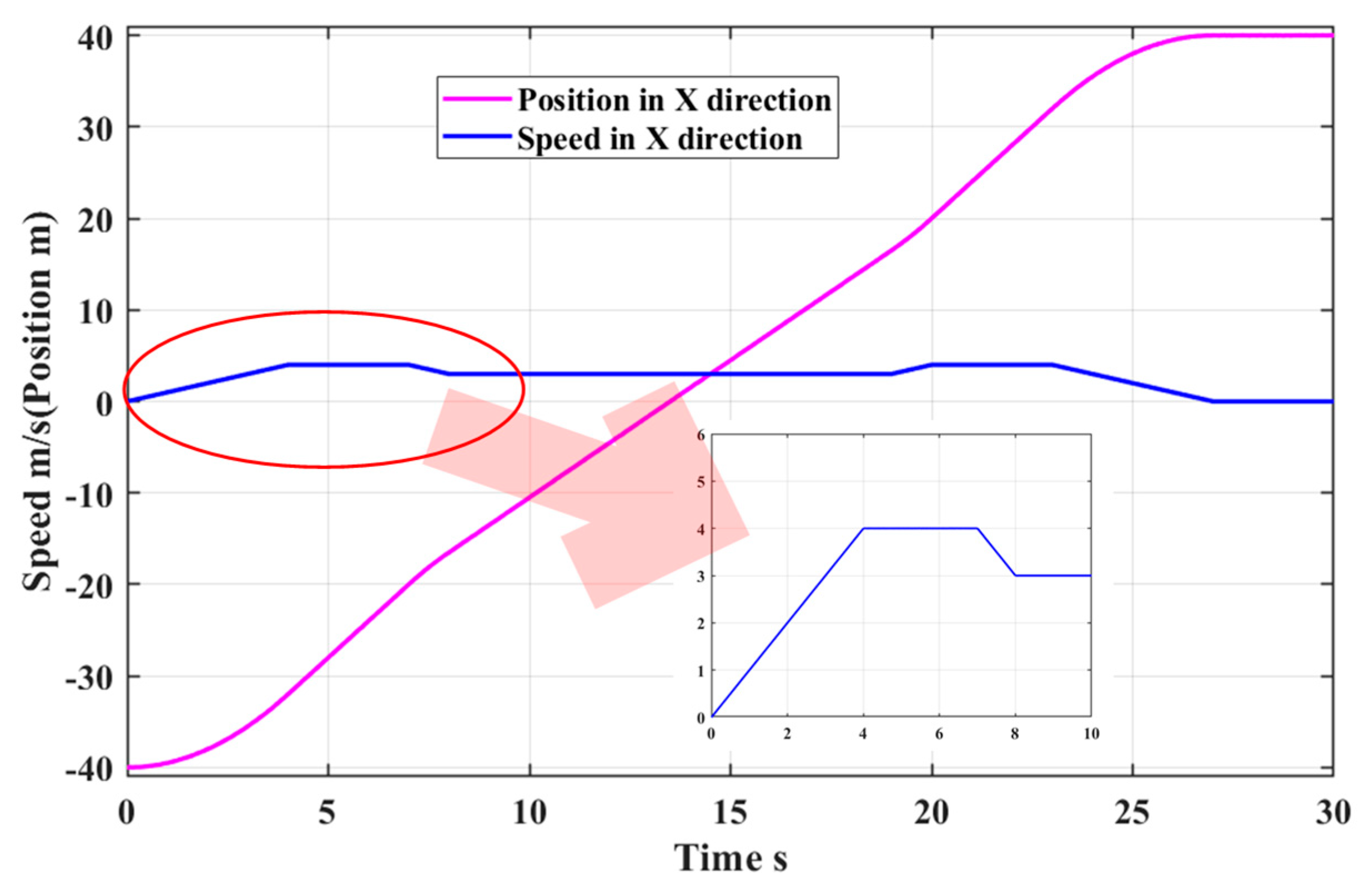
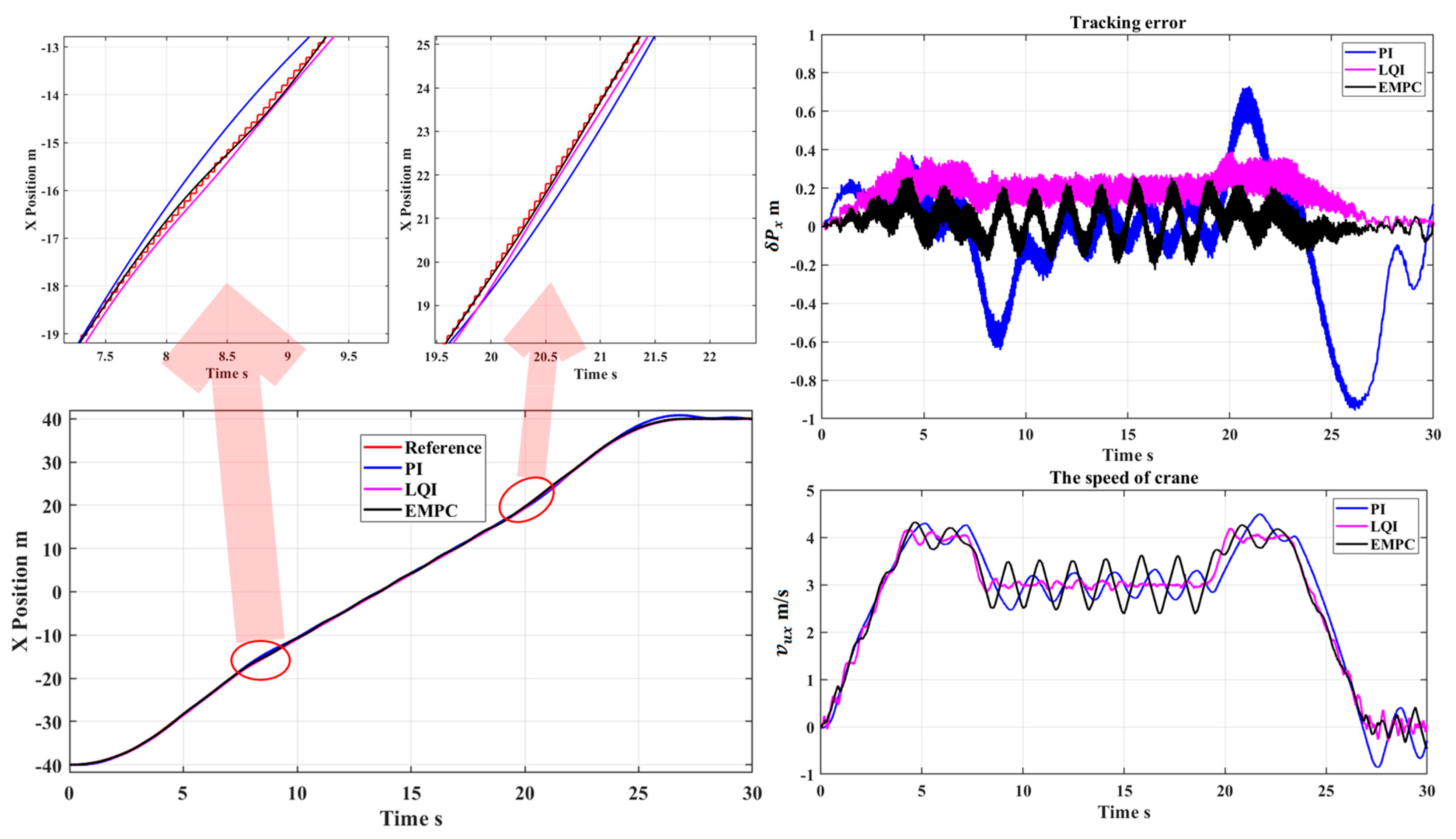
Figure 9 presents a comparison of simulation results for track-following servo control along path one, using three different controllers: PI, LQI, and EMPC. The “Reference” curve shows the real-time position of the CLRV. The figure displays the tracking results, tracking errors, and the crane speed of the track-following servo for each controller.
It can be observed from
Figure 9 that the EMPC controller has the best performance and the smallest tracking error against the disturbance caused by the rapid change in the
X-direction speed of the CLRV, followed by the LQI and PI controllers. Moreover, by examining the motion speed diagram of the crane, it can be inferred that the tracking stability of LQI is highest.
As shown in
Figure 9, the positional deviation resulting from the track-following servo of the PI controller is significantly greater than those of the EMPC and LQI controllers. This is primarily due to the high inertia of the crane, which poses challenges in tracking the desired path. To overcome this, a simple PI controller with higher proportional coefficients is employed, leading to improved response speed but degraded steady-state performance. Interestingly, LQI has a lower settling time than PI and EMPC, and its stability is best. This can be attributed to its very high weight in the state of the tracking error, which helps it reach the steady state earlier. However, LQI suffers from delay errors between the desired path and the crane position, resulting from its reliance on the output value of the error integrator.
In contrast, the EMPC controller enhances control performance by generating optimal inputs while satisfying constraints. The model predictive control algorithms used in EMPC are more complex, taking into account various parameters and predicting the most optimal path for possible trajectories. As a result, the EMPC controller performs better at minimizing errors compared to controllers that use a simple cost function or a set of gains to correct deviations.
Figure 9 shows the tracking error of tracking desired path one using the EMPC controller.
refers to the real-time error of the crane and lunar rover in the
X direction, while
refers to the real-time error of the trolley and lunar rover in the
Y direction. In the tracking servo of path one, there is only an error in the
X direction. The tracking error
and the tracking error of the EMPC controller for path one is within 0.2 m.
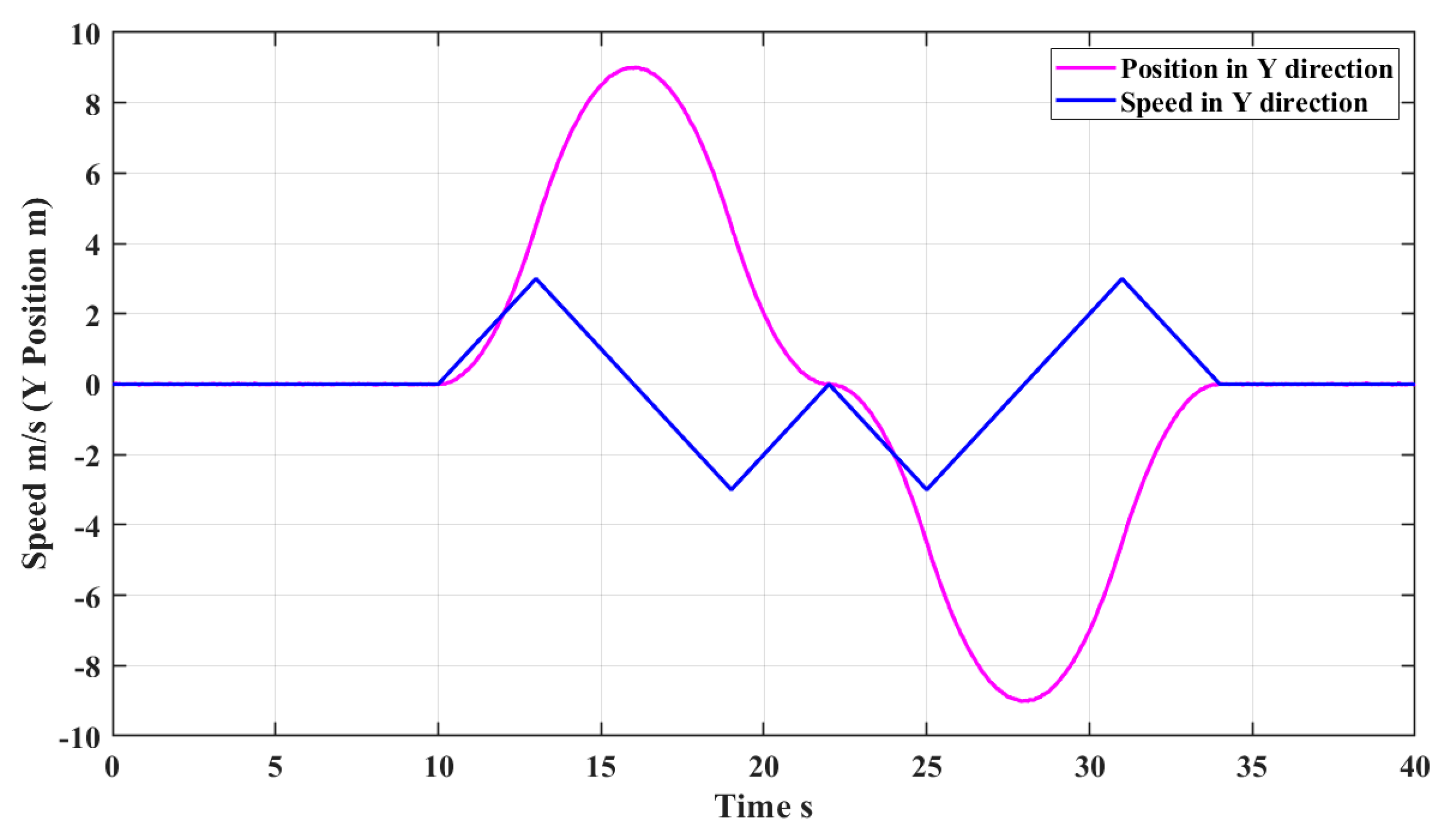
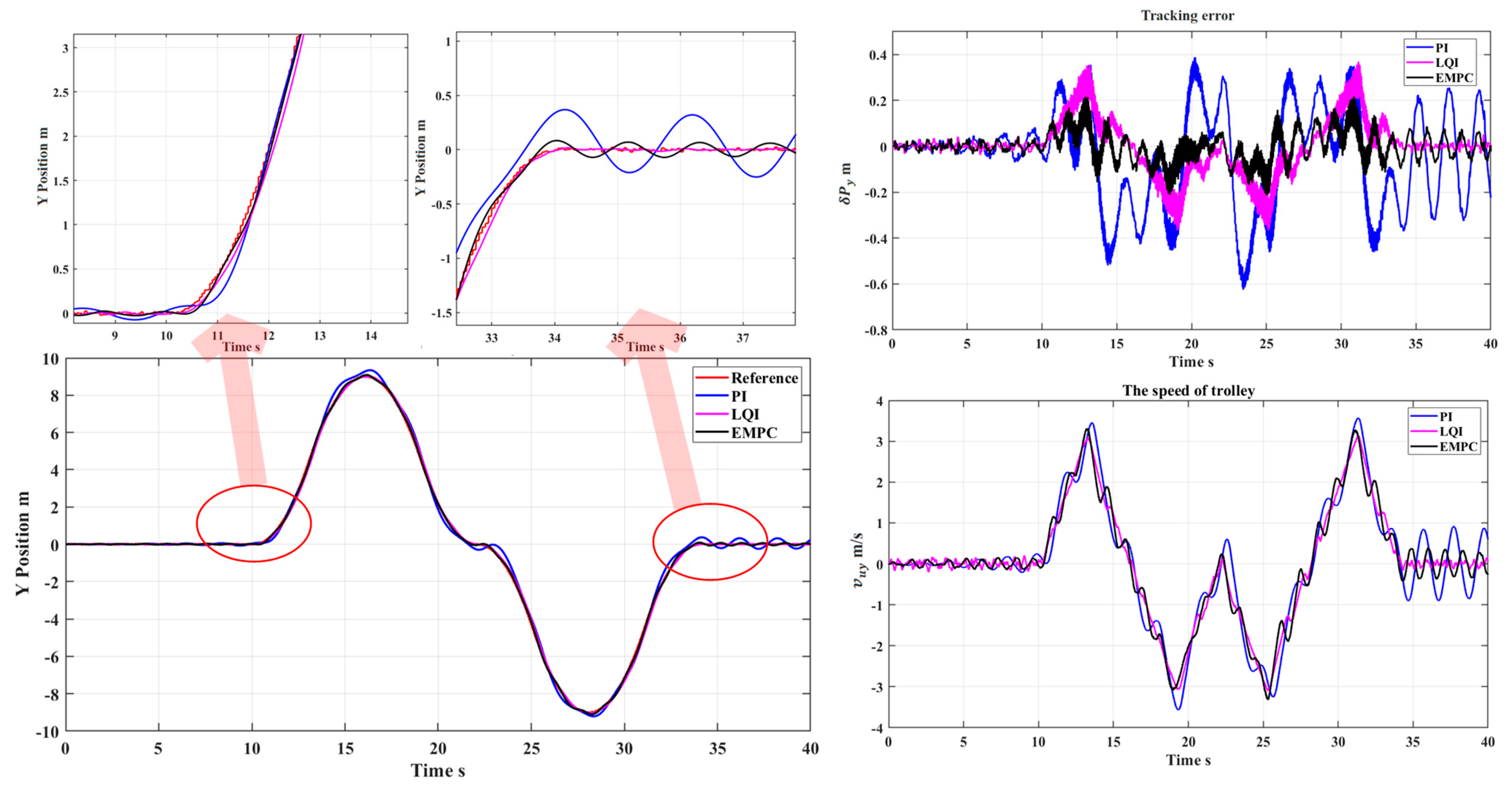
Figure 10 depicts the simulation results of the trolley tracking path two, which involves frequent acceleration, deceleration, and forward and reverse movements in the
Y direction.
Figure 10 shows the simulation results of the trolley tracking path two in the
Y direction. The tracking error is mainly caused by the trolley’s inertia. Comparing it with
Figure 9, it can be observed that as the crane’s inertia is much greater than that of the trolley, the error will be even greater when the crane tracks the expected path with rapid changes in the
X-directional speed. The results shown in
Figure 10 show the trolley’s speed
of tracking path two. From the tracking error plot and trolley speed plot, it can be seen that large errors usually occur during the time periods when the trolley undergoes acceleration and deceleration switching. To minimize the impact of the crane’s large inertia on tracking performance, it is recommended to avoid frequent acceleration and deceleration of the lunar rover in the
X direction. Instead, it is advisable to conduct forward and reverse movement performance testing solely in the
Y direction to achieve optimal results.
In the tracking servo of path two, there is only an error in the Y direction. The tracking error and the tracking error of the EMPC controller for path two is within 0.2 m.
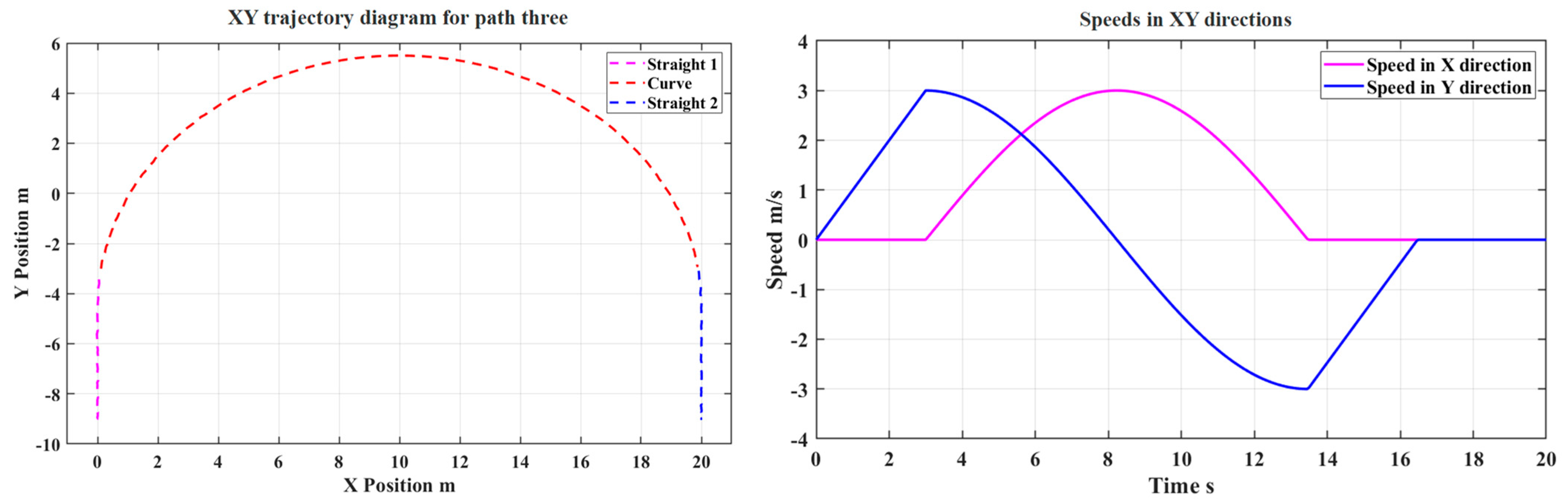
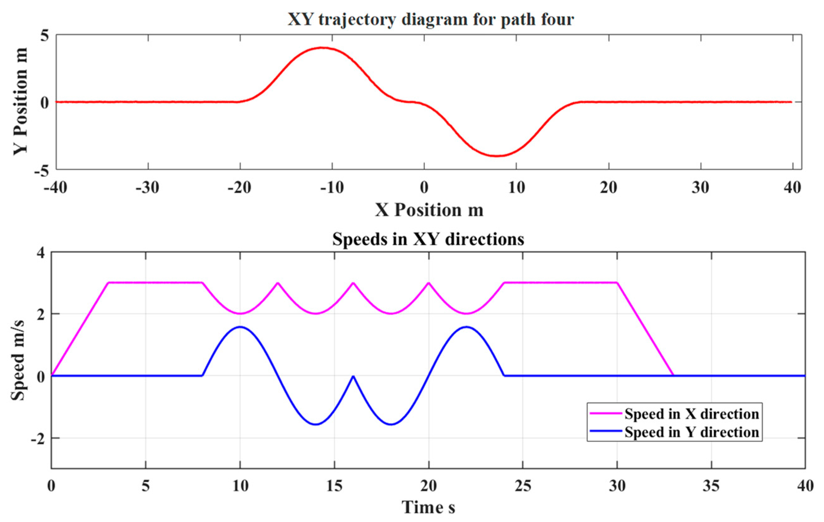
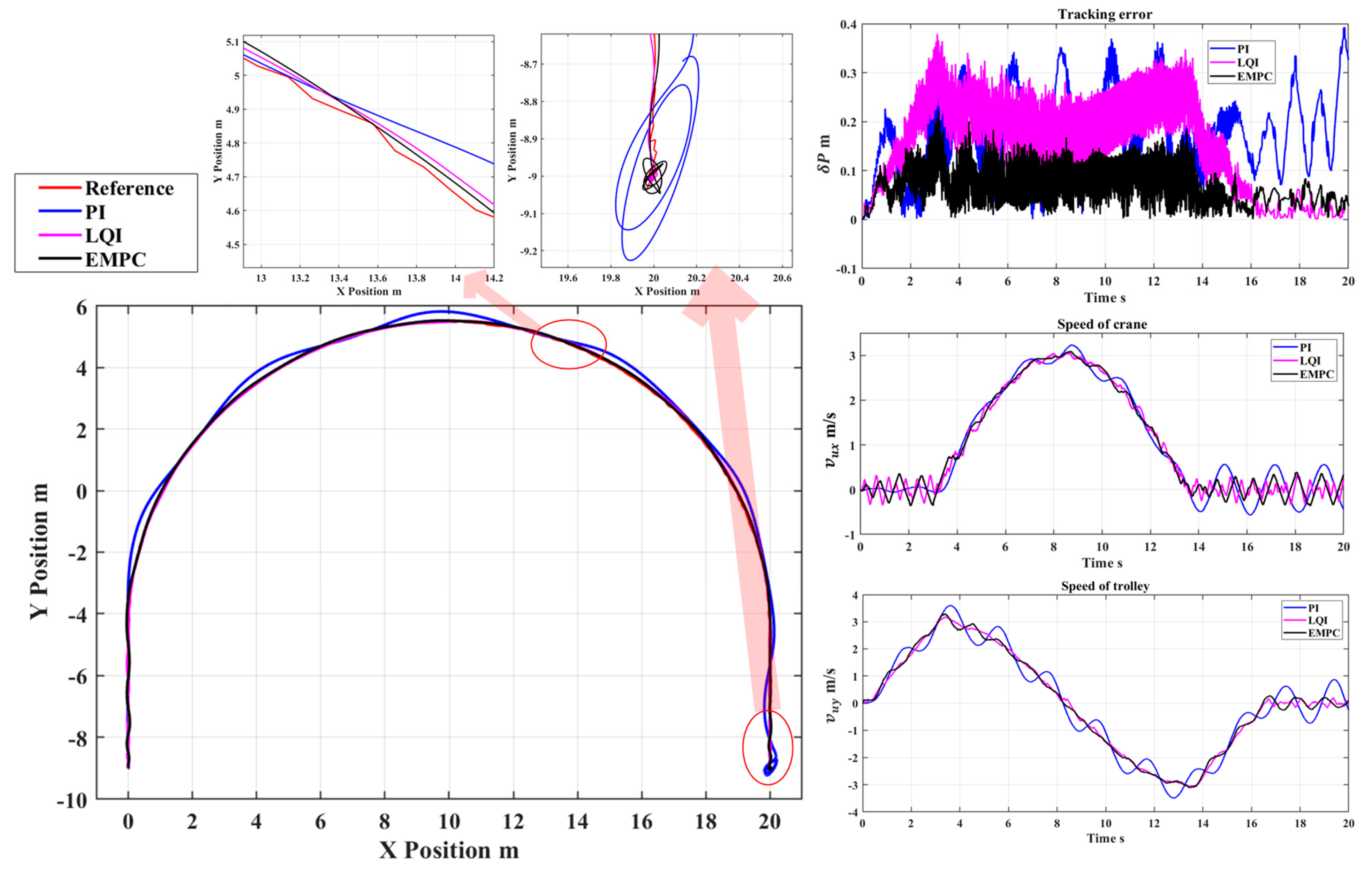
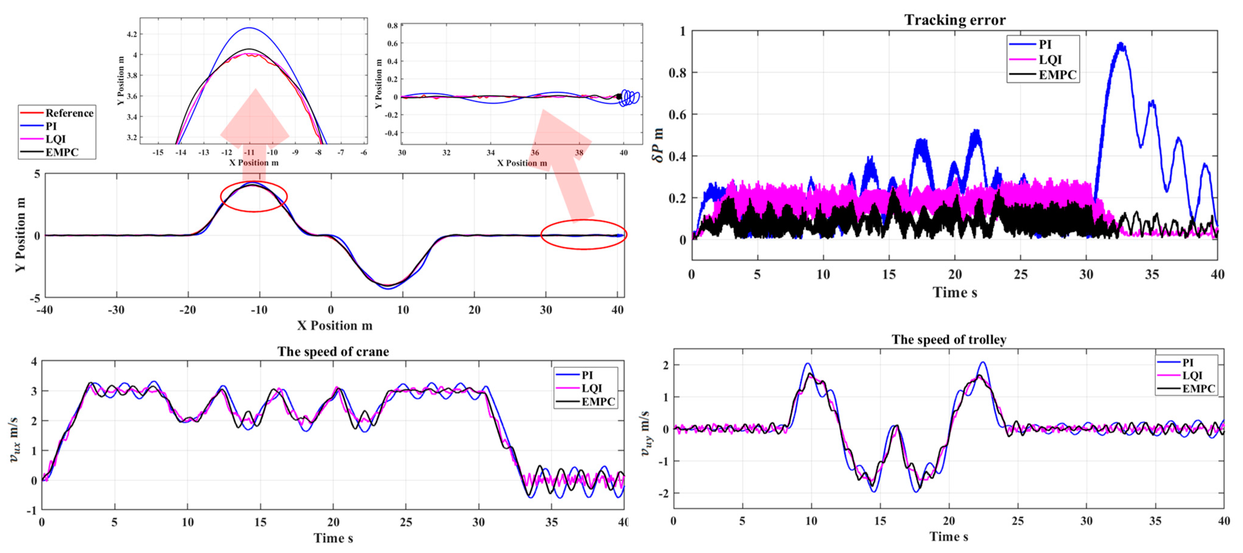
Figure 11 depicts the simulation results of the crane and trolley tracking desired path three, which follows a turning motion trajectory of the CLRV with a radius of 10 m, and operates at a speed of 3 m/s. On the other hand,
Figure 12 illustrates the crane and trolley tracking path four, which represents the driving trajectory of the CLRV when encountering continuous turns during obstacle avoidance. The CLRV operates at a speed of around 3 m/s while following this path.
Figure 11 and
Figure 12 illustrate that the EMPC controller results in the smallest tracking error, followed by LQI and PI controllers. Furthermore, the results suggest that the LQI controller exhibits excellent stability, as the movement speed of the crane and trolley remains relatively stable in response to dynamic disturbances. On the other hand, when using a PI controller for a large inertia system, the overshoot can be relatively large, and it can be challenging to balance the response speed and stability.
Figure 11 and
Figure 12 displays the simulation results of crane and trolley tracking for desired paths three and four, utilizing the EMPC controller. The tracking error
is basically less than 0.2 m.
The simulation results show that the maximum tracking errors
of the track-following servo subsystem using EMPC controllers are almost less than 0.2 m. According to Equations (39) and (40), it can obtain the influence factor of the tracking error on the CLRV motion in the horizontal direction:
In addition, the error impact factor in the vertical direction is as follows:
The simulations yield some key findings: the EMPC demonstrates a notably impressive performance for the system, with explicit MPC delivering the objectively best results. While the PI and LQI controllers show comparatively inferior results, they remain reliable options with their own strengths. The PI controller is easy to apply, while the LQI controller exhibits excellent robustness and stability. However, their application is limited for multi-constraint control systems. Although the EMPC shows good performance under different expected trajectories, it also has some limitations in terms of stability, especially in dealing with large disturbances in the X direction (i.e., when the CLRV speed changes rapidly). In such cases, the crane may lose control. To address this issue, future work will focus on conducting relevant methods to further analyze the stability of the proposed EMPC controller.
In conclusion, EMPC is a controller that can provide the smallest possible dynamic tracking error and steady-state error under the condition of dealing with multiple constraints, and it has better control performance. Moreover, frequent acceleration and deceleration should be avoided in the X direction when driving the CLRV, to reduce the impact of the large inertia of the crane on the controller’s tracking performance.
Based on the simulation results, we compare the tracking performance of the track-following servo subsystem of the suspension gravity compensation system to that of the system designed by Liu et al. [
2]. Although the maximum tracking error of Liu et al.’s system is approximately 0.1 m, its crane employs open-loop control, making it only suitable for tracking a slow-moving unmanned lunar rover. In contrast, the research presented in this paper provides a solution to the theoretical research gap of the track-following servo subsystem suitable for CLRV experiments.
6. Conclusions
This paper proposes a design and control scheme for a track-following servo subsystem of a LGCS suitable for CLRV ground testing:
The track-following servo subsystem consists of a crane, trolley, and servo motors. The crane moves along the bridge, tracking the real-time position of the CLRV, while the trolley moves along the crane girder to follow the real-time position of the CLRV. Three-loop control models are established for both the crane and trolley, including the position loop, motor speed loop, and current loop.
The driving force of the track-following servo subsystem is provided by a PMSM. Specific parameters for the motor and transmission mechanism are determined based on the subsystem’s motion capability. PMSM vector control based on the SVPWM is adopted to achieve fast response and precise control of the motor speed. PI controllers are employed in both the current and speed loops of the motors.
In the position loop control of the track-following servo subsystem, explicit MPC control is introduced for multi-parameter constraint control. This paper presents an EMPC controller suitable for the track-following servo subsystem, including the cost function design and offline calculation process. The weighting matrices, prediction horizon, and control horizon are also determined.
Especially, the effectiveness of the proposed EMPC controller is demonstrated through a comparison with PI and LQI controllers. The simulation results show that the maximum tracking error of the track-following servo subsystem is consistently below 0.2 m. The impact of the errors on the drawbar pull is within 12.5%, and their effect on the compensation force is negligible. The simulation results also suggest that, due to the large inertia of the crane, the CLRV should avoid frequent forward, backward, acceleration, and deceleration in the X direction to reduce the influence of the crane’s large inertia on tracking performance. These simulation results provide valuable theoretical support for designing a track-following servo subsystem that is suitable for CLRV ground testing.
In our future work, our objective is to develop a track-following servo subsystem that is suitable for ground testing of the CLRV. The primary contribution of this paper is the development of an EMPC controller for the position control loop, along with PMSM vector control, which has demonstrated excellent tracking performance for the subsystem. However, implementing the EMPC controller in engineering settings may pose significant challenges. In our upcoming research, we plan to refine our work further, including addressing potential deviations in motor load torque, exploring cooperative control of multiple motors, and enhancing the robustness of the EMPC controller. These are essential considerations that must be addressed to fully realize the potential of the proposed approach in practical applications.


