Boundary–Inner Disentanglement Enhanced Learning for Point Cloud Semantic Segmentation

Abstract

In a point cloud semantic segmentation task, misclassification usually appears on the semantic boundary. A few studies have taken the boundary into consideration, but they relied on complex modules for explicit boundary prediction, which greatly increased model complexity. It is challenging to improve the segmentation accuracy of points on the boundary without dependence on additional modules. For every boundary point, this paper divides its neighboring points into different collections, and then measures its entanglement with each collection. A comparison of the measurement results before and after utilizing boundary information in the semantic segmentation network showed that the boundary could enhance the disentanglement between the boundary point and its neighboring points in inner areas, thereby greatly improving the overall accuracy. Therefore, to improve the semantic segmentation accuracy of boundary points, a Boundary–Inner Disentanglement Enhanced Learning (BIDEL) framework with no need for additional modules and learning parameters is proposed, which can maximize feature distinction between the boundary point and its neighboring points in inner areas through a newly defined boundary loss function. Experiments with two classic baselines across three challenging datasets demonstrate the benefits of BIDEL for the semantic boundary. As a general framework, BIDEL can be easily adopted in many existing semantic segmentation networks.

1. Introduction

Semantic information is the key to understanding the virtual scene constructed by a point cloud [1] in applications such as indoor navigation [2], autonomous driving [3], and cultural heritage [4]. Advances in the current semantic segmentation networks are due to various delicate designs of local aggregation operators (LAOs), which generally take the features and coordinates of the center point and its neighboring points as input, outputting the transformed feature for the center point [5]. Nevertheless, most LAOs aggregate the features of all neighboring points equally, thus smoothing the extracted features on the semantic boundary, which results in a bad contour for final semantic segmentation. Here, the semantic boundary refers to the transitional area between objects with different categories. For example, the joint where the window meets the wall can be defined as the boundary (the points not on the boundary make up the inner areas), as shown in the red regions in Figure 1.

There are a few boundary-related methods for point cloud semantic segmentation [6,7,8,9,10,11,12]. IAF-Net [6] adaptively selects indistinguishable points such as boundary points and improves the segmentation performance of these points through multistage loss. JSENet [7] adds a semantic edge detection stream, which outputs the semantic edge map and jointly learns the semantic segmentation and semantic edge. BoundaryAwareGEM [8] constitutes a boundary prediction module to predict the boundary, utilizing the predicted boundary to generate LAO aggregate features with discrimination. PushBoundary [9] consists of two streams for prediction of the boundary and the direction of the interior, thus guiding boundaries to their original locations. Most of these methods rely on additional boundary prediction modules, thus increasing model complexity. Unlike existing works, this paper is motivated by the goal of improving the segmentation accuracy of boundary points without requiring additional modules and learning parameters.

Figure 1. Visualization of boundary generated from ground-truth image. Each scene was selected from S3DIS [13]. Red outlines represent boundary areas.

Figure 1. Visualization of boundary generated from ground-truth image. Each scene was selected from S3DIS [13]. Red outlines represent boundary areas.

It is well known that endowing a point cloud with boundary information can help improve the overall segmentation accuracy [12]. The boundary information can change the segmentation result by affecting features learned by the network. To explore the role of the boundary, this paper analyzes the change in feature similarity between the boundary point and its neighboring points utilizing the boundary information. Specifically, for every boundary point, its neighboring points are partitioned into four collections in terms of two factors: whether they are on the boundary, and whether their categories are the same as the center point. Then, the entanglement between the boundary point and each collection of neighboring points is measured, representing their proximity in the representation space. Results show that the boundary can weaken the boundary–inner entanglement, where “boundary–inner” represents the boundary point and its neighboring points in inner areas. It is shown that reducing the boundary–inner entanglement is beneficial for improving the segmentation accuracy.

Therefore, to improve the segmentation accuracy of boundary points, a lightweight Boundary–Inner Disentanglement Enhanced Learning (BIDEL) framework is proposed, which can maximize the boundary–inner feature distinction through a newly defined boundary loss function $L_{BIDEL}$. Boundary information is only utilized in the loss function at the training stage; thus, BIDEL does not need additional modules for explicit boundary prediction. Experiments with two classic baselines across three datasets demonstrate that BIDEL can assist the baseline in obtaining a better accuracy of boundary points and small objects.

In summary, the following key contributions are highlighted:

(1)

This paper shows that reducing boundary–inner entanglement is beneficial for overall semantic segmentation accuracy.

(2)

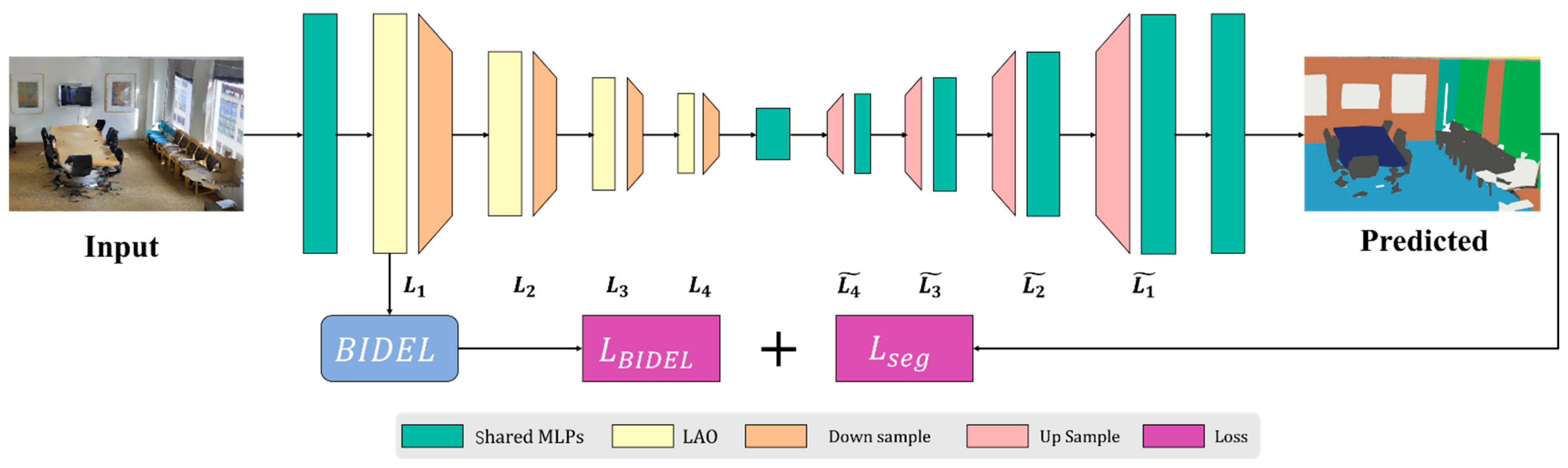
This paper proposes BIDEL, a lightweight framework for improving the segmentation accuracy of boundary points, which can maximize boundary–inner disentanglement through a newly formulated boundary loss function. Notably, BIDEL does not need additional complex modules and learning parameters, and it can be integrated into many existing segmentation networks.

(3)

Experiments on challenging indoor and outdoor benchmarks show that BIDEL can bring significant improvements in boundary and overall performance across different baselines.

The remainder of this paper is organized as follows: semantic segmentation methods based on deep learning, especially those related to boundaries, are reviewed in Section 2; the proposed BIDEL is described in Section 3; the experimental results are presented and discussed in Section 4; lastly, the conclusions are summarized in Section 5.

2. Related Work

2.1. Semantic Segmentation

Semantic segmentation of a point cloud is aimed at assigning each 3D point to an interpretable category. Recently, methods based on deep learning have gradually replaced traditional methods that rely on handcrafted features. They can automatically learn high-dimensional features, realizing end-to-end semantic classification. These methods can be classified into three types based on input data formats: voxel-based [14,15,16,17,18], multi-view-based [19,20,21,22,23,24,25,26], and point-based [27,28,29,30,31,32,33,34].

To process 3D data, one typical approach is to store the point cloud in voxel grids and apply 3D convolution directly [14]. However, limited by acquisition techniques, the points in the point cloud are usually not distributed homogeneously, making most voxel grids unoccupied. Therefore, an unmodified dense 3D convolution on sparse grids is inefficient. To solve this problem, SS-CNs [15] was proposed as a sparse convolution operator to deal with sparse point clouds more efficiently. On the other hand, OctNet [16] partitions 3D space hierarchically using a set of unbalanced octrees, allowing more memory and computation resources to be allocated to relatively dense regions. This achieves a deeper network without prohibitive high resolution. However, transforming a point cloud into voxels is both memory-unfriendly and computation-inefficient, and this process can inevitably discard a lot of geometric information. Another approach is to project the point cloud into multiple views on which the de facto standard 2D convolution can be adopted directly [19,20,21,22,23,24,25,26]. However, this kind of method is highly independent on projection position and angle, thus becomes a suboptimal choice for large-scale point cloud semantic segmentation.

PointNet [33] pioneered the original research on point clouds without any data transformations. It independently learns point features with pointwise multilayer perceptions (MLPs). Despite being permutation-invariant, it fails to capture local context and performs poorly on complex scenes. PointNet++ [34] was a further optimization of PointNet. It adopts hierarchical multiscale feature aggregation structures to extract local features, which can significantly improve the overall accuracy. It also provides a de facto standard paradigm for subsequent segmentation networks, which mostly comprise subsampling, LAO, and up-sampling modules. RSNet [35] splits the point cloud into many ordered slices along the x-, y-, and z-axes, on the basis of which global features are pooled. Then, the learned orderly feature vectors are processed with a recurrent neural network. However, such MLP-based methods do not fully consider the relationship between points and their local neighbors, limiting their ability to capture local contexts [36]. It is well known that local contextual information is crucial for dense tasks, such as semantic segmentation. Recently, much effort has been made for effective LAOs, enabling researchers to explore and make the most of local relationships. Among them, pseudo-grid-based methods [31,37,38,39] and adaptive-weight-based methods [28,30,40,41] are widely used. Akin to 2D convolution for image pixels, pseudo-grid-based methods associate the weight matrix with predefined kernel points. However, the pseudo-kernel points must be defined artificially, which limits model generalizability and flexibility on different datasets. In contrast, adaptive-weight-based methods learn the convolution weight from features and the relative position relationship through MLPs.

Although these delicately designed LAOs work well, experiments have shown that they already describe the local context sufficiently with saturated performance [42]. Therefore, this paper turns to another direction, focusing on semantic boundaries, which are usually overlooked in current segmentation networks.

2.2. Semantic Boundary

In 2D image vision tasks, boundaries were initially a concern, especially in the medical field [43,44]. However, few studies noted the impact of semantic boundaries on holistic point cloud segmentation. Research has shown that boundary points are more likely to be misclassified than those in inner areas [12]. Therefore, it is very important and challenging to improve performance on the semantic boundary. GAC [40] learns the convolution weights from the feature differences between the center point and its neighboring points, thus guiding the convolution kernel to distinguish the boundary location. The boundary areas delineating skeletons provide basic structural information, while the extensive inner areas depicting surfaces supply the geometric manifold context. Therefore, GDANet [45] divides the holistic point cloud into high-frequency (contour) components and low-frequency (flat) components, paying attention to different types of components when extracting geometric features, so that the network can capture and refine their complementary geometries to supplement local neighboring information. BEACon [10] designs a boundary embedded attentional convolution network, where the boundary is expressed through geometric and color changes to influence the convolution weights. These studies considered the boundary implicitly in segmentation backbones.

IAF-Net [6] categorizes areas that are hard to be segmented into three types: boundary areas, confusing interior areas, and isolated small areas. It can adaptively select points in these areas and specifically refine their learned features. It is well known that semantic boundaries cannot been adopted a priori at the testing stage. Therefore, to utilize boundary information explicitly, one common workaround is to add an extra boundary prediction module (BPM) to predict the semantic boundary, and then use these predictions as auxiliary information in the segmentation backbone. To prevent the local features of different categories from being polluted by one another, an independent BPM module was proposed in [8] to predict point cloud boundaries. The predicted boundary information is utilized as an auxiliary mask to assign different weights to different points during feature aggregation, thus preventing the propagation of features across boundaries. JSENet [7] jointly learns the semantic segmentation and semantic edge detection tasks. However, these methods are not suitable for unstructured environments, which usually feature unclear semantic edges. To this end, the authors of [11] designed cascaded edge attention blocks to extract high-resolution edge features, and then fused the extracted edge features with semantic features extracted by the main segmentation branch. These methods utilize boundary information explicitly to improve performance on the boundary, but the newly embedded boundary prediction modules greatly increase complexity. On the other hand, the numbers of boundary points and inner points vary hugely, which is a challenge for binary boundary/inner classification. To improve performance on the boundary with no need for complex modules, CBL [12] optimizes the representations learned by LAOs through contrastive learning on the boundary point, enhancing its similarity with neighboring points belonging to the same category in the representation space. However, it ignores the relationship between the boundary point and its neighboring points in inner areas.

Unlike the abovementioned studies, this paper explores the relationship between the boundary point and its neighboring points in inner areas, proposing a lightweight framework for improving the segmentation accuracy of boundary points with no need for additional modules.

3. Methods

Firstly, to explore the role of the boundary, the change in entanglement between the boundary point and its neighboring points after utilizing boundary information is analyzed (Section 3.1). It is found that the boundary can greatly reduce boundary–inner entanglement and help improve the overall semantic segmentation accuracy. Then, BIDEL is proposed for improving the segmentation accuracy of boundary points (Section 3.2), which can enhance boundary–inner disentanglement through a boundary loss function $L_{BIDEL}$. Lastly, the implementation details such as semantic segmentation baselines and network parameter settings are presented in Section 3.3.

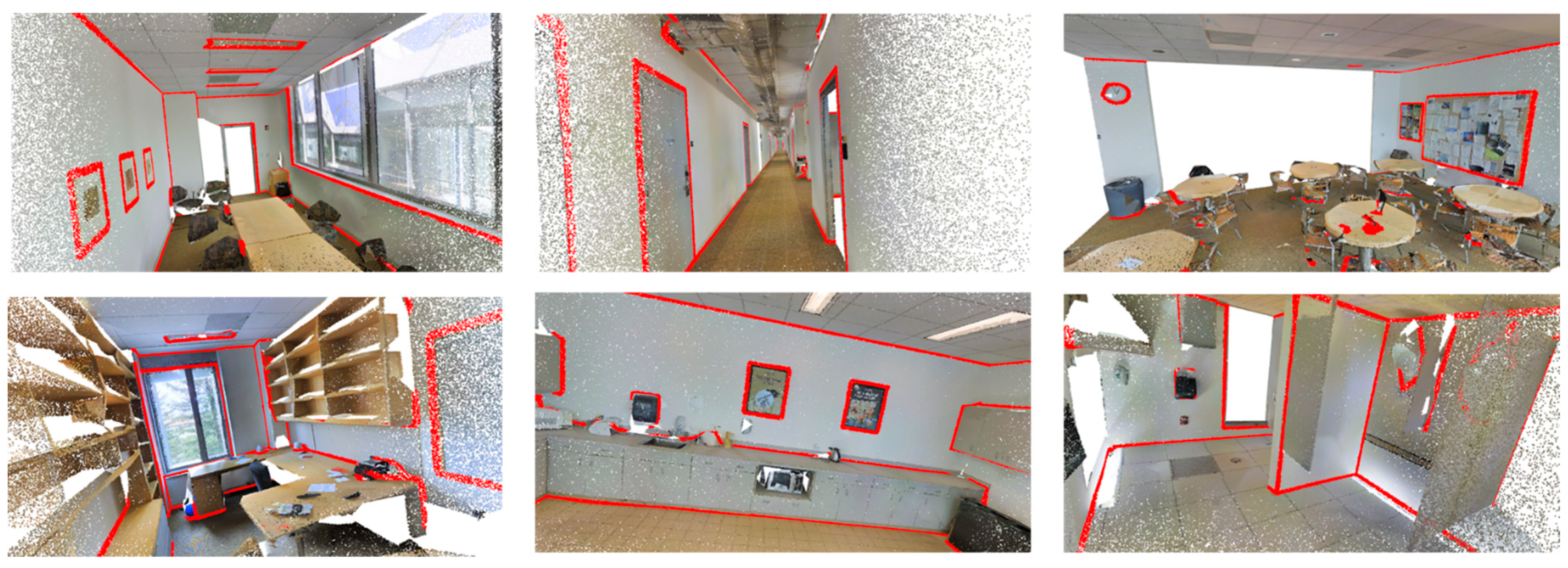
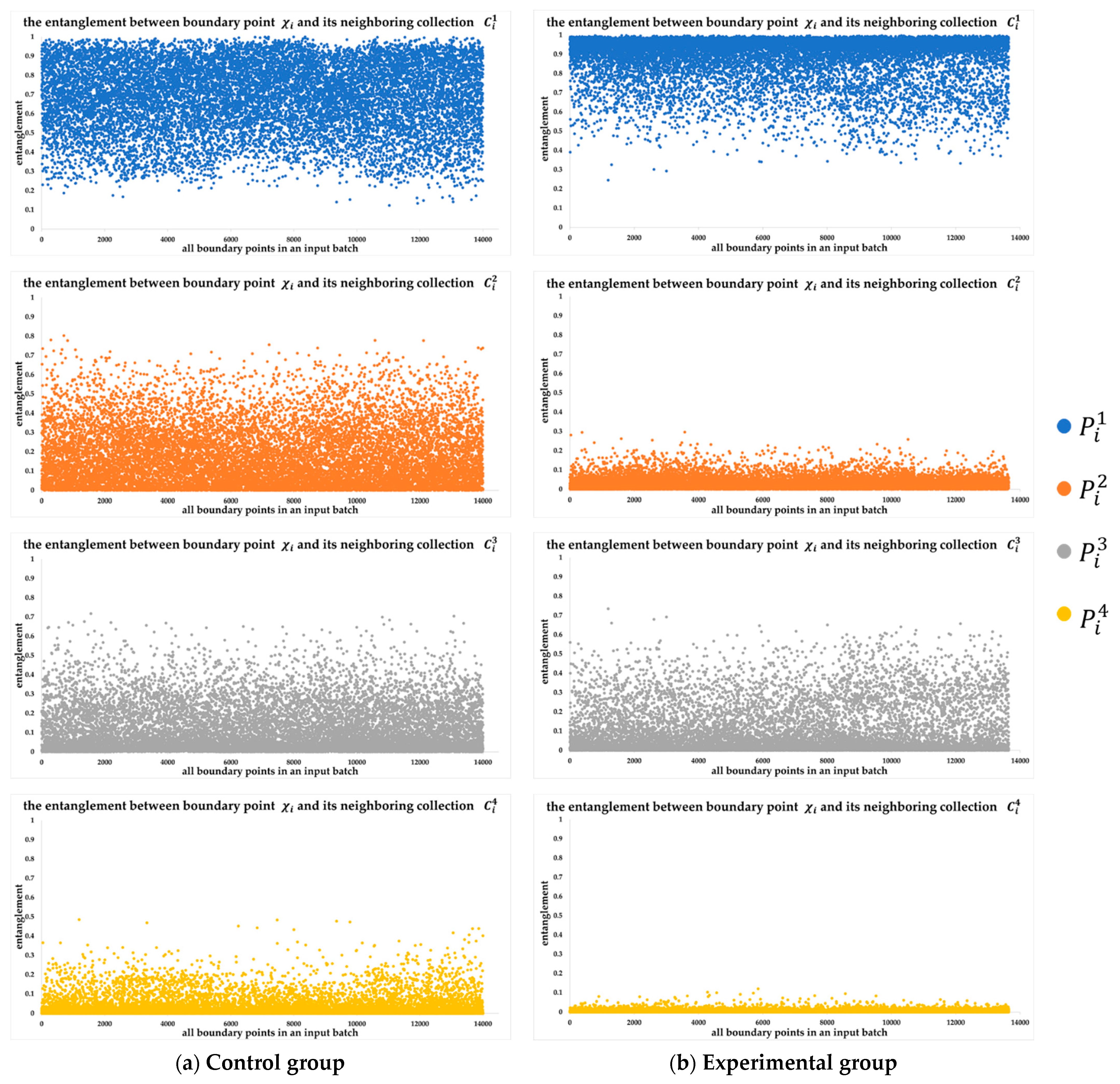
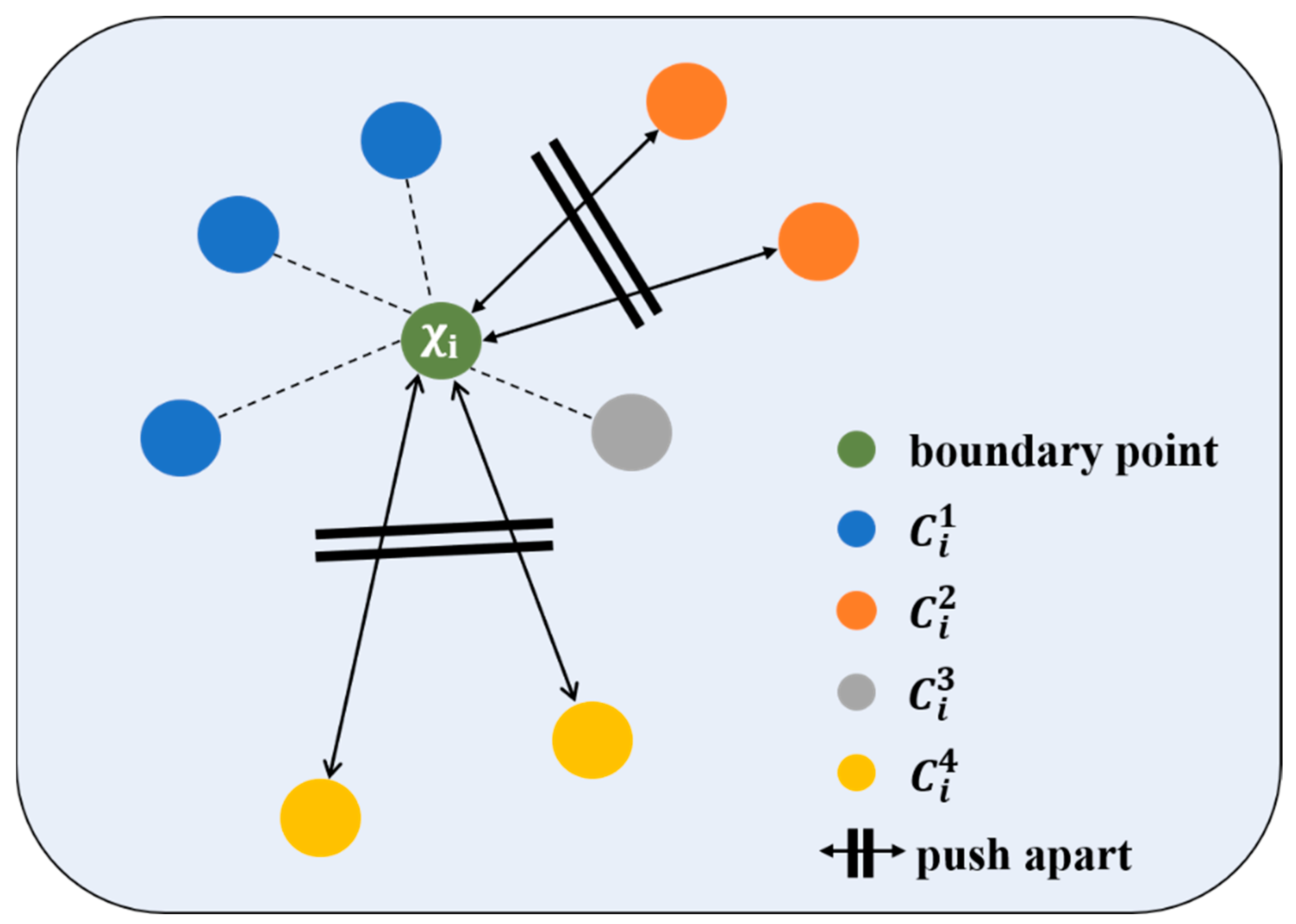
3.1. Boundary–Inner Entanglement Measurement

Consider a point cloud with n points, denoted by ${\rm X}=\{{\chi }_1,\cdots ,{\chi }_i,\cdots ,{\chi }_n|{\chi }_i=\left(p_i,f_i\right),p_i\in R^3,f_i\in R^d\}$, where $p_i=\left(x_i,y_i,z_i\right)$ represents Euclidian 3D coordinates, $f_i$ represents additional feature attributes such as color, surface normal, and intensity, and d represents feature dimensions. With point ${\chi }_i$ as a centroid, its neighboring points $N_i$ are identified using the simple K-nearest neighbors (KNN) algorithm. A point ${\chi }_i$ is annotated as a boundary point if there exists a point in a different category in the neighborhood; otherwise, it is annotated as an inner point. Accordingly, a boundary point set $B_l$ can be generated from the ground truth:

$$B_l=\left\{{\chi }_i\in {\rm X}|\exists {\chi }_k\in N_i,l_k\ne l_i\right\},$$

(1)

where $l_i$ represents the ground truth of the center point ${\chi }_i$.

Some basic variables involved in this paper are summarized as follows:

• ${\rm X}$ denotes the input point cloud;
• n denotes the number of points in ${\rm X}$;
• ${\chi }_i$ denotes point $i$ in ${\rm X}$;
• $l_i$ denotes the ground truth of ${\chi }_i$;
• $p_i=\left(x_i,y_i,z_i\right)$ denotes the Euclidian 3D coordinates of ${\chi }_i$;
• $f_i$ denotes the feature of ${\chi }_i$;
• $B_l$ denotes the boundary point set in ${\rm X}$.

For training the point cloud with the ground truth, its boundary information @boundary is generated according to Equation (1). As shown in Figure 1, the generated boundaries (red regions) are located at the joints between objects belonging to different categories, delineating a clear semantic contour of the 3D objects. Specifically, $@{\mathrm{boundary}}_i$ is equal to 1 if point ${\chi }_i$ belongs to $B_l$; otherwise, it is equal to 0.

Table 1. The semantic segmentation results of S3DIS Area1 on RandLA-Net [28]. Bold font in the table body denotes the best performance.

	Input	OA (%)	mACC (%)	mIoU (%)
Control group	(x, y, z, r, g, b)	88.7	85.9	74.4
Experiment group	(x, y, z, r, g, b, @boundary)	93.0	90.5	81.6

compares the segmentation results of the control group and experimental group, where the control group takes the initial point cloud as input, whereas the experimental group takes the point cloud endowed with boundary information as input. The mean intersection over union (mIoU), overall accuracy (OA), and mean class accuracy (mACC) are used as evaluation metrics to quantitatively compare the results of the different methods, which are respectively computed as

$$\mathrm{mIoU}=\frac{1}{S}{\displaystyle \sum }_{s=1}^S\frac{{\sum }_{{\chi }_i\in {\rm X}}\left[pre{d}_i=s\wedge l_i=s\right]}{{\sum }_{{\chi }_i\in {\rm X}}\left[pre{d}_i=s\vee l_i=s\right]},$$

(2)

$$\mathrm{OA}=\frac{{\sum }_{{\chi }_i\in {\rm X}}\left[pre{d}_i=l_i\right]}{n},$$

(3)

$$\mathrm{mACC}=\frac{1}{S}{\displaystyle \sum }_{s=1}^S\frac{{\sum }_{{\chi }_i\in {\rm X}}\left[pre{d}_i=s\wedge l_i=s\right]}{{\sum }_{{\chi }_i\in {\rm X}}\left[l_i=s\right]},$$

(4)

where $S$ represents the total number of classes, $pre{d}_i$ represents the predicted label of point ${\chi }_i$, $[\cdot ]$ represents a Boolean function that outputs 1 if the condition within $[\cdot ]$ is true and 0 otherwise.

As can be seen, the experimental group achieved the better mIoU of 81.6%. To explore the role of the boundary, the change in entanglement between boundary point and its neighboring points is analyzed. The detailed steps are as follows:

Partition the neighboring points into four collections. For a center point ${\chi }_i\in B_l$, its neighboring points are partitioned into four collections from the perspective of two factors: whether they are on the boundary, and whether their categories are the same as ${\chi }_i$. The four collections are as follows:

(1)

$C_i^1=\{{\chi }_k\in N_i | l_k=l_i \wedge {\chi }_k\in B_l\}$: boundary points within the same category;

(2)

$C_i^2=\{{\chi }_k\in N_i | l_k=l_i \wedge {\chi }_k\notin B_l\}$: inner points within the same category;

(3)

$C_i^3=\{{\chi }_k\in N_i | l_k\ne l_i \wedge {\chi }_k\in B_l\}$: boundary points in a different category;

(4)

$C_i^4=\{{\chi }_k\in N_i | l_k\ne l_i \wedge {\chi }_k\notin B_l\}$: inner points in a different category.

Measure the entanglement between boundary point to its each collection. Inspired by [46,47], the soft nearest loss without negative logarithm function is used to measure the entanglement. For a boundary center point ${\chi }_i\in B_l$, its entanglement with $C_i^j$ is defined by $P_i^j$:

$$P_i^j=\frac{{\sum }_{{\chi }_k\in N_i\wedge {\chi }_k\in C_i^j}exp\left(-\parallel f_i-f_k\parallel \right)}{{\sum }_{{\chi }_k\in N_i}exp\left(-\parallel f_i-f_k\parallel \right)}, 0\le P_i^j\le 1,$$

(5)

where $\parallel \cdot \parallel$ represents the $L_2$ Euclidean distance. A larger $P_i^j$ denotes stronger entanglement between point ${\chi }_i$ and its neighboring collections $C_i^j$. $B_l$ is generated from the ground truth of the input point cloud, and the boundary feature is a kind of low-level local feature that can be extracted by LAO. Therefore, $f_i$ refers specifically to the internal representation learned by the LAO in the first encoding stage, where the point cloud has not yet been subsampled. In the LAO, greater affinity between the center point ${\chi }_i$ and its neighboring point results in a greater corresponding convolution weight and denotes more similar transformed features. Entanglement essentially represents feature the similarity between point pairs. Therefore, the metric $P_i^j$ can be intuitively described as the degree of attention between point ${\chi }_i$ and its neighboring collections $C_i^j$.

Compare the measuring results. The measuring results are plotted in Figure 2. Comparing the plots by column, in the control group (Figure 2a), $P_i^1>P_i^2>P_i^3>P_i^4$ on average, indicating that the boundary point is more entangled with its neighboring points in the same category, whereas, in the experimental group (Figure 2b), $P_i^1>P_i^3>P_i^2>P_i^4$ on average, indicating that the boundary point is more entangled with its neighboring points on the boundary. Comparing the plots by row, $P_i^2$ and $P_i^4$ decreased greatly in the experimental group.

It was speculated that the boundary acts as a barrier in the LAO, where it prevents the boundary point from focusing on neighboring points in inner areas. Due to the role of the boundary, relatively more attention is paid to neighboring collections $C_i^1$ or $C_i^3$ (boundary points when put together), such that boundary feature is preserved and, subsequently, the overall performance is improved. In summary, the entanglement between boundary point ${\chi }_i$ and its neighboring collections $C_i^2$ or $C_i^4$ (inner points when put together) are weakened greatly after utilizing boundary information. This shows that reducing boundary–inner entanglement is beneficial for semantic segmentation accuracy.

3.2. Boundary–Inner Disentanglement Enhanced Learning

According to the measurement results from Section 3.1, a lightweight Boundary–Inner Disentanglement Enhanced Learning (BIDEL) framework for improving the segmentation accuracy of boundary points is proposed. Specifically, BIDEL maximizes the boundary–inner feature distinction through the boundary loss function $L_{BIDEL}$:

$$L_{BIDEL}=-\frac{1}{\left|B_l\right|}{\sum }_{{\chi }_i\in B_l}log\left(P_i^1+P_i^3\right),$$

(6)

where $\left|·\right|$ represents the number of points. $L_{BIDEL}$ maximizes the sum of $P_i^1$ and $P_i^3$, as a result of which the sum of $P_i^2$ and $P_i^4$ is minimized, and the boundary–inner disentanglement is enhanced. As shown in Figure 3, BIDEL pushes neighboring collections $C_i^2$ (points in orange) and $C_i^4$ (points in yellow) apart, thus preserving the boundary by preventing it from being contaminated by the features of inner points, which improves the segmentation accuracy of boundary points in particular.

Notably, the boundary information generated from the ground truth is only used for network training; therefore, an additional boundary prediction module is not required.

$L_{BIDEL}$ is added to the final loss function as a regularizer, through which the model can achieve two training objectives: (1) minimize the overall segmentation cross-entropy loss; (2) minimize boundary–inner entanglement. The final loss function is

$$L=L_{cross entrophy}+\lambda L_{BIDEL},$$

(7)

where $\lambda$ is the loss weight of $L_{BIDEL}$.

3.3. Implementation Details

Current segmentation networks generally follow the encoder–decoder paradigm, where different LAOs and subsampling strategies are used in encoding layers to extract multilevel local features, skip connections, and up-sampling operations employed in decoding layers to achieve end-to-end semantic segmentation. LAOs can be classified into three types: MLP-based, pseudo-grid-based, and adaptive-weight-based [5]. The latter two types have become the mainstream due to their excellent local feature extraction ability. Pseudo-grid-based methods preplace some pseudo-kernel points in the neighborhood and learn their convolutional weights directly. However, the pseudo-kernel points must be defined artificially, which can limit the generalizability and flexibility of models. In contrast, adaptive-weight-based methods learn convolutional weights indirectly from the relative position and features of the center point and its neighboring points. KPConv [31] and RandLA-Net [28] are classic representatives of pseudo-grid-based methods and adaptive-weight-based methods, respectively. Both follow the encoder–decoder paradigm. RandLA-Net obtains a lower segmentation accuracy than KPConv, but has a marked drop in memory overhead and computation cost due to the mechanism of random sampling.

To validate the benefits of the proposed BIDEL across different LAOs, this paper refers to KPConv and RandLA-Net as baselines. The overall architecture is depicted in Figure 4, where BIDEL is applied to optimize the representations learned by LAO in the first encoding layer.

This paper sets the loss weight λ = 1 for $L_{BIDEL}$, and ten follows the same training settings as the baselines for fair comparisons. Specifically, for KPConv, the optimizer, initial learning rate, and maximum training epoch are set to Momentum, 0.01, and 500, respectively; for RandLA-Net, the optimizer, initial learning rate, batch size, maximum training epoch, and the number of nearest points are set to Adam, 0.01, 4 × 40,960, 100, and 16, respectively.

The mIoU, OA, and mACC are considered as the evaluation metrics to quantitively demonstrate the benefits of BIDEL, in line with most point cloud semantic segmentation works. The experimental configurations are detailed in

Table 2. The hardware and software configurations for the experiments.

		Configuration
Hardware	CPU	AMD Ryzen 9 5900X 12-Core Processor 3.70 GHz
	GPU	NVIDIA GeForce RTX 3080 Ti
Software	Python IDE	Pycharm
	Deep learning library	Tensorflow
	Visualization	Cloud Compare

.

4. Experimental Results and Discussion

In this section, we evaluate the benefits of BIDEL with two baselines across three large-scale public datasets, S3DIS [13] (Section 4.1), Toronto-3D [48] (Section 4.2), and Semantic3D [49] (Section 4.3), before demonstrating its effectiveness through ablation analysis (Section 4.4).

4.1. S3DIS Indoor Scene Segmentation

S3DIS [13] is an indoor dataset with high quality, recorded by a Matterport camera. The whole dataset has around 273 million points annotated with 13 semantic labels. It consists of six large areas. Area 5 is used for validating and testing, which follows common practice [12,28]. The experimental results are compared with baselines and some classic studies in

Table 3. Quantitative results on S3DIS Area 5. The red font denotes obvious better results (greater than 1%) than baseline. Bold font denotes the best result among all methods. * These methods consider boundaries.

Methods	mIoU (%)	OA (%)	mACC (%)	Ceil.	Floor	Wall	Beam	Col.	Wind.	Door	Table	Chair	Sofa	Book.	Board	Clut.
PointNet [33]	41.1	-	49.0	88.8	97.3	69.8	0.1	3.9	46.3	10.8	59.0	52.6	5.9	40.3	26.4	33.2
SegCloud [50]	48.9	-	57.4	90.1	96.1	69.9	0.0	18.4	38.4	23.1	70.4	75.9	40.9	58.4	13.0	41.6
PointCNN [29]	57.3	85.9	63.9	92.3	98.2	79.4	0.0	17.6	22.8	62.1	74.4	80.6	31.7	66.7	62.1	56.7
SPG [51]	58.0	86.4	66.5	89.4	96.9	78.1	0.0	42.8	48.9	61.6	84.7	75.4	69.8	52.6	2.1	52.2
GAC [40]	62.9	87.8	-	92.3	98.3	82.0	0.0	20.4	59.0	40.9	85.8	78.6	70.8	61.7	74.7	52.8
PCT [27]	61.3	-	67.7	92.5	98.4	80.6	0.0	19.4	61.6	48.0	76.6	85.2	46.2	67.7	67.9	52.3
IAF-Net * [6]	64.6	88.4	70.4	91.4	98.6	81.8	0.0	34.9	62.0	54.7	79.7	86.9	49.9	72.4	74.8	52.1
JSENet * [7]	67.7	-	-	93.8	97.0	83.0	0.0	23.2	61.3	71.6	89.9	79.8	75.6	72.3	72.7	60.4
PushBoundary * [9]	67.1	89.7	-	94.0	97.9	82.6	0.0	23.3	56.6	75.4	80.1	91.1	75.7	74.4	62.3	59.1
CBL * [12]	65.3	87.5	74.5	92.2	97.7	81.0	0.0	36.8	61.0	39.4	78.1	88.1	81.4	71.5	68.7	52.6
KPConv [31]	66.2	-	-	94.8	98.4	82.9	0.0	18.0	53.4	67.1	83.0	91.4	63.8	75.5	71.6	60.8
+BIDEL *	67.0	-	-	94.9	98.5	83.3	0.0	21.4	54.9	68.5	83.1	91.2	66.0	75.7	71.8	61.1
RandLA-Net [28]	62.7	87.5	71.1	92.3	97.8	80.7	0.0	19.5	59.2	46.8	78.0	85.7	63.2	70.9	68.0	53.0
+BIDEL *	64.7	88.0	73.6	93.0	96.1	81.5	0.0	28.8	62.7	43.9	74.0	87.0	72.6	71.9	73.7	55.8

. The results of methods other than KPConv and RandLA-Net were directly cited from public reports. It can be seen that KPConv improved the mIoU by 0.8% and RandLA-Net improved the mIoU by 2% after being integrated with BIDEL, showing the effectiveness and generalizability of BIDEL in different LAOs. With BIDEL, KPConv obtained the leading performance of 94.9% for ceiling, 83.3% for wall, 75.7% for bookstore, and 61.1% for clutter. Notably, considerable gains were achieved over RandLA-Net for small objects such as sofa (+9.4%), column (+9.3%), and board (+5.7%). Although the improvements of BIDEL were inferior to those of other boundary-related methods such as JSENet [7] (+2.3%) and CBL [12] (+2.9%), BIDEL can be considered superior due to its simplicity without increasing model parameters. For example, JSENet designs a semantic edge detection stream to explicitly predict the edge, which greatly increases the number of parameters; CBL applies contrast boundary learning to the input point cloud and each subscene point cloud. However, if contrast boundary learning is only applied to the input point cloud, as performed in BIDEL, the relative improvement compared to baseline is much lower than that of BIDEL.

Furthermore, the benefits of BIDEL for KPConv and RandLA-Net are qualitatively demonstrated in Figure 5 and Figure 6, respectively. Misclassification usually appears in transition areas. For example, in Figure 6, in the second row, third column, points of the “clutter” category and “ceiling” category are poorly separated; in the fifth row, third column, the chair cannot be identified accurately when put together with the table. By contrast, BIDEL performs well in these transition areas. The overall improved areas are consistent with the semantic boundaries.

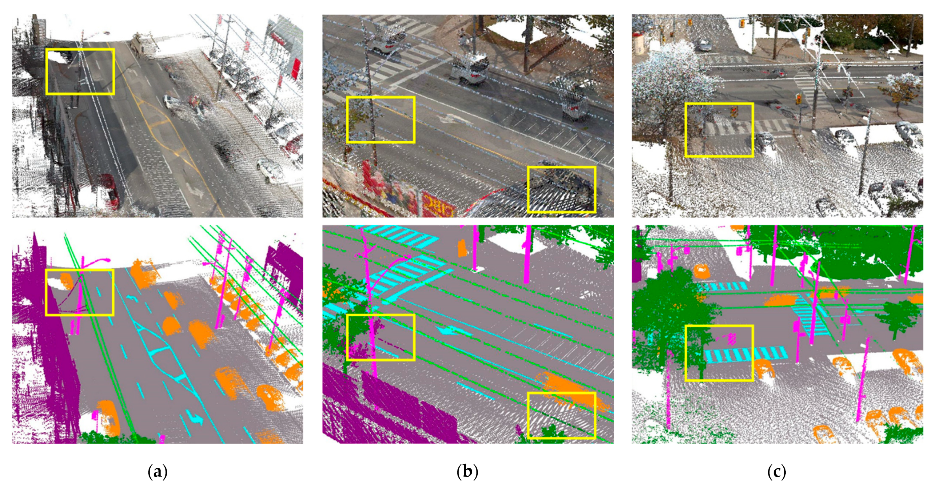
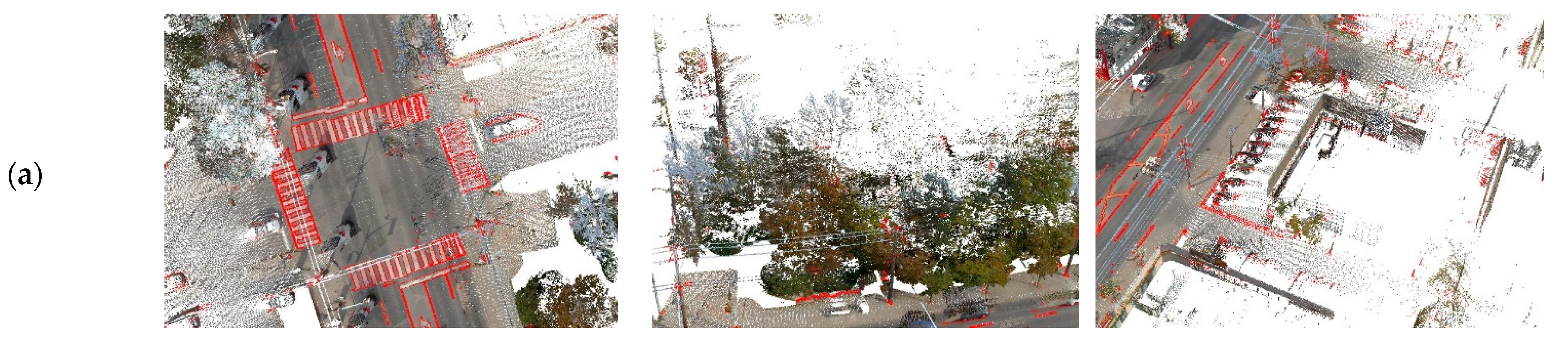
4.2. Toronto-3D Outdoor Scene Segmentation

This paper also demonstrates the generalizability of BIDEL using an outdoor dataset, Toronto-3D [48]. This is a large-scale urban outdoor point cloud dataset acquired by the MLS system in Toronto, Canada, covering about 1 km of point clouds and consisting of about 78.3 million points belonging to one of eight classes, such as road markings and cars. It covers four blocks. The L002 scene was selected for validation and testing, whereas the other scenes were selected for training. This dataset is labeled inaccurately in some areas. For example, objects that should be utility lines are labeled as buildings (Figure 7a) or trees (Figure 7b), while objects that should be poles are labeled as natural (Figure 7c). Although each point provides rich attributes such as xyz coordinates, rgb colors, intensity, GPS time, scan angle rank, and class label, this experiment only used the xyz and rgb attributes, following the same settings as used for S3DIS. There were some challenges when performing the semantic segmentation task: (1) objects belonging to the pole/natural/utility line categories often overlapped with each other; (2) road markings were small and narrow objects.

Table 4. Quantitative results on Toronto-3D benchmark. The red font denotes better results (greater than 0.5%) than the baseline. Bold font denotes the best result among all methods. * These methods consider boundaries.

Input	Methods	mIoU(%)	OA(%)	Road	Road Marking	Natural	Building	Utility Line	Pole	Car	Fence
xyz	PointNet++ [34]	41.8	84.9	89.3	0.0	69.0	54.1	43.7	23.3	52.0	3.0
	DGCNN [41]	61.8	94.2	93.9	0.0	91.3	80.4	62.4	62.3	88.3	15.8
	KPConv [31]	69.1	95.4	94.6	0.1	96.1	91.5	87.7	81.6	85.7	15.7
	MS-PCNN [52]	65.9	90.0	93.8	3.8	93.5	82.6	67.8	72.0	91.1	22.5
	MS-TGNet [48]	70.5	95.7	94.4	17.2	95.7	88.8	76.0	74.0	94.2	23.6
	RandLA-Net [28]	77.7	93.0	94.6	42.6	96.9	93.0	86.5	78.1	92.9	37.1
	Multi-Loss PointNet++ [53]	71.0	83.6	92.8	27.4	89.9	95.3	85.6	74.5	44.4	58.3
	MappingConvSeg [54]	82.9	94.7	97.2	67.9	97.6	93.8	86.9	82.1	93.7	44.1
xyz, rgb	KPConv [31]	81.4	-	97.9	74.9	96.6	91.6	87.1	81.7	94.8	26.9
	+BIDEL *	82.0	-	97.9	76.3	97.5	92.5	87.5	82.6	95.1	26.2
	RandLA-Net [28]	81.1	96.3	95.5	56.8	96.2	93.1	88.0	82.2	88.2	48.4
	+BIDEL *	81.5	96.7	96.1	61.3	97.0	93.5	87.3	81.2	90.1	45.3

summarizes the evaluation results and quantitative comparisons. BIDEL showed a slight improvement over the baselines, with obvious gains in the road marking (+4.5%) and car (+1.9%) categories based on RandLA-Net. With BIDEL, KPConv achieved the leading performance of 97.9% for roads, 76.3% for road markings, 82.6% for poles, and 95.1% for cars. Figure 8 visualizes the segmentation results. It is evident that the improved areas aligned with the boundary contours. For example, as shown in the first column, RandLA-Net tended to broaden the width of road markings, whereas BIDEL outlined the boundaries more accurately. Compared to outdoor Toronto-3D scenes, objects were labeled in more detail and connected more densely in indoor scenes such as S3DIS [7], resulting in more semantic boundary points, enabling the effectiveness of BIDEL to be adequately demonstrated. Therefore, fewer gains were obtained for the Toronto-3D dataset.

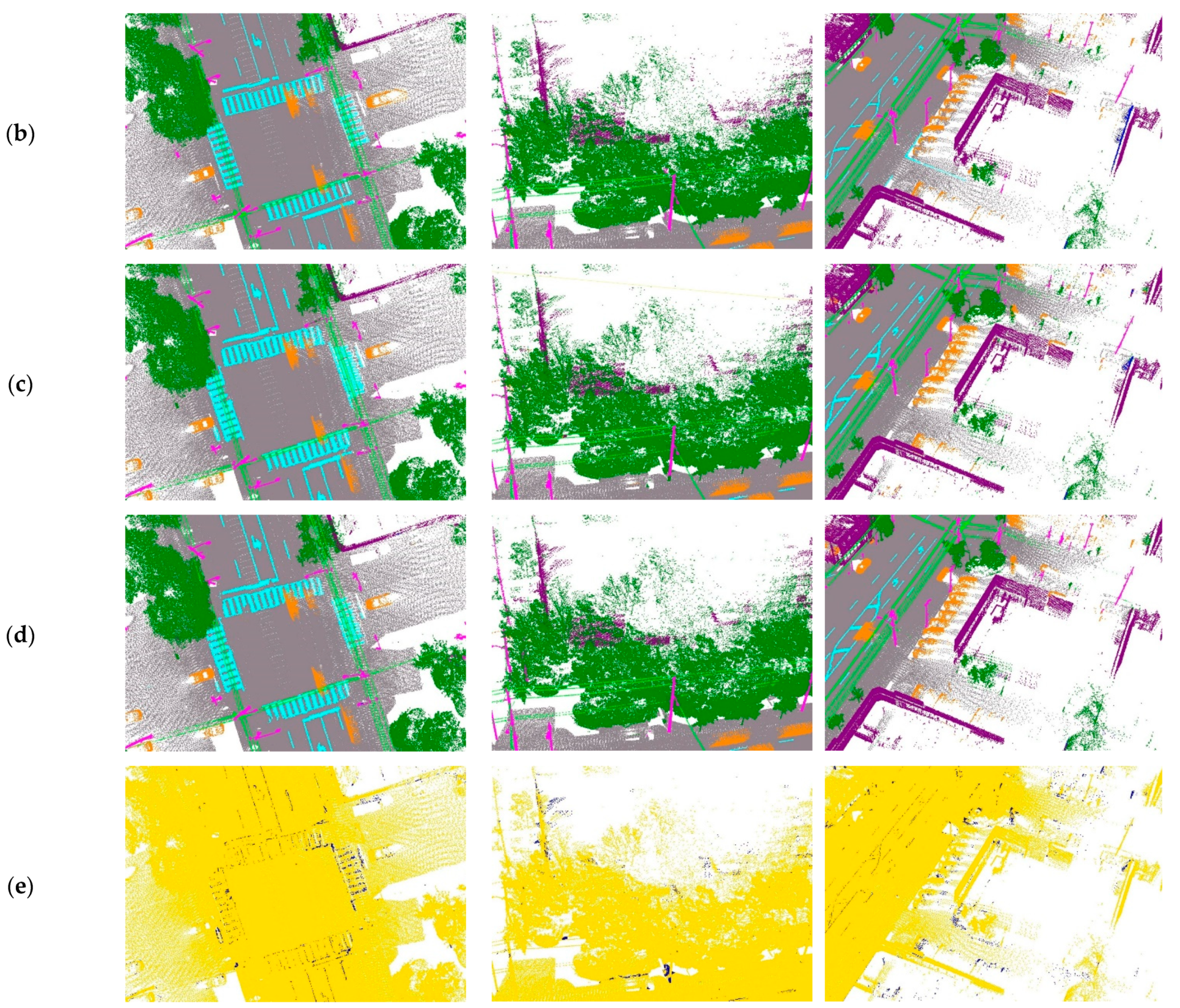
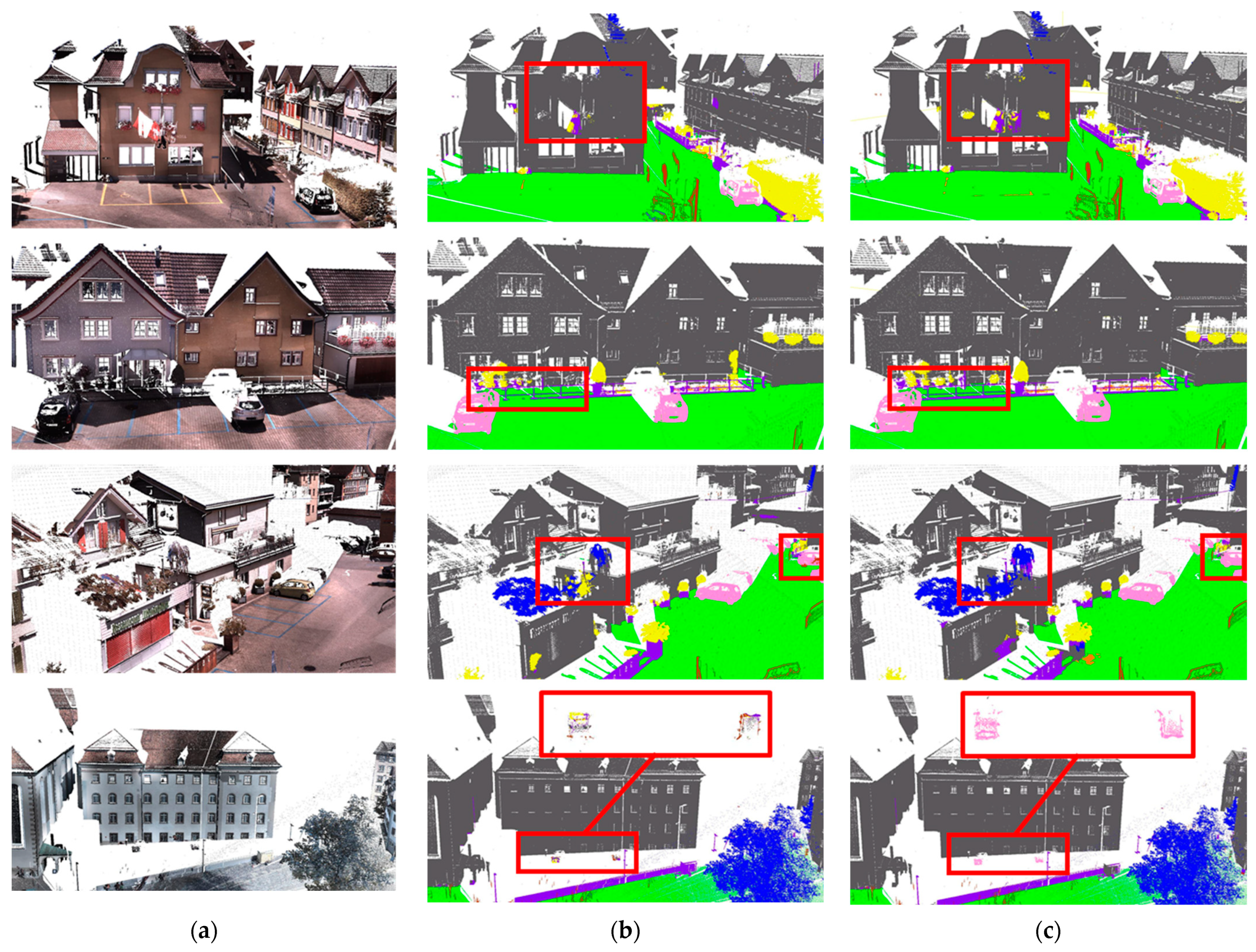
4.3. Semantic3D Outdoor Scene Segmentation

Semantic3D [49] is a large-scale outdoor dataset with over four billion points. It provides 15 scenes for training and four for testing, with each point assigned to one of eight labels such as buildings and cars. Misclassified boundaries are likely to cause misidentification of small objects such as cars, which would be catastrophic for autonomous driving applications. In Semantic3D, low vegetation and cars are both small objects, while low vegetation usually exists on building balconies, making the recognition of these two classes challenging. By contrast, BIDEL performed well for small objects such as low vegetation and cars, as shown in Figure 9. For example, as shown in the fourth row, the baseline did not identify cars at all, whereas BIDEL achieved this successfully. Improvements in these two classes prove the power of the proposed method for semantic boundaries.

4.4. Ablation Analysis

Effectiveness of BIDEL. The proposed BIDEL can maximize the feature similarity between boundary points and its neighboring points on the boundary ($C_i^1$ and $C_i^3$), thus preserving the boundary and boosting segmentation accuracy. However, CBL [12] encourages the learned representations of boundary points more similar to their neighboring points within the same category ($C_i^1$ and $C_i^2$) in decoding layers. Therefore, several different boundary loss functions are discussed in this section to prove the effectiveness of BIDEL.

For the first loss function setting, the learned representations of boundary point ${\chi }_i$ are encouraged to be more similar to its neighboring collections $C_i^1$ (boundary points within the same category), which can be represented as $L_A$:

$$L_A=-\frac{1}{\left|B_l\right|}{\sum }_{{\chi }_i\in B_l}log\left(P_i^1\right).$$

(8)

For the second loss function setting, the learned representations of boundary point ${\chi }_i$ are encouraged to be more similar to its neighboring collections $C_i^1$ and $C_i^2$ (points within the same category), which can be represented as $L_B$:

$$L_B=-\frac{1}{\left|B_l\right|}{\sum }_{{\chi }_i\in B_l}log\left(P_i^1+P_i^2\right).$$

(9)

As shown in

Table 5. The quantitative results of different boundary loss functions for semantic segmentation. Bold font denotes the best performance.

Boundary Loss	mIoU (%)	OA (%)	mACC (%)
$L_A$	64.5	87.5	72.5
$L_B$	62.2	86.7	71.7
$L_{BIDEL}$	64.8	87.8	72.9

, when setting $L_A$ as the boundary loss function, the mIoU reached 64.5%, showing a 1.8% increase compared to the baseline. $L_{BIDEL}$ achieved the best result of 64.8%. Points in collection $C_i^3$ only accounted for a small proportion of all neighboring points, which limited the effect of BIDEL and resulted in a slight improvement in accuracy. However, $L_B$ unfortunately diminished the accuracy. Compared to $L_A$, $L_B$ also encouraged entanglement between the boundary point and its neighboring collections $C_i^2$ (inner points within the same category). This shows that a high engagement of inner points in LAO can weaken the boundary information, thus reducing overall performance. Such observations successfully verify the effectiveness of BIDEL.

Hyperparameter optimization. Three values of $\lambda$ were evaluated to select the best loss weight for $L_{BIDEL}$. The experiments were conducted on S3DIS Area 5, and the results are reported in

Table 6. Quantitative results with different values of $\lambda$. Bold font denotes the best performance.

$\mathit{\lambda }$	mIoU (%)	OA (%)	mACC (%)
0.5	64.0	87.4	72.5
1	64.8	87.8	72.9
5	63.4	87.7	71.2

. It can be seen that $\lambda =1$ was the best choice.

5. Conclusions

This paper proposed a novel lightweight BIDEL framework that can improve the semantic segmentation accuracy of boundary points. The results in this paper revealed that reducing boundary–inner entanglement is beneficial for overall accuracy; accordingly, BIDEL was proposed, which uses a boundary loss function to maximize boundary–inner disentanglement. Compared with the current boundary-related networks that rely on complex modules and increase model complexity, BIDEL does not require additional modules or learning parameters. On a large-scale indoor dataset with more semantic boundaries, BIDEL significantly improved the overall segmentation accuracy, especially for small objects. On large-scale outdoor datasets with fewer semantic boundaries, the visualization results showed that the improved areas approximately aligned with the semantic boundaries. Both quantitative and qualitative experimental results demonstrated the better effect of BIDEL on semantic boundaries.

Due to the excellent performance of BIDEL on boundary points, semantic segmentation networks integrated with BIDEL can improve indoor navigation, automatic driving, and other application scenarios containing small objects or rich semantic boundaries, thereby obtaining a more accurate semantic contour.

However, this research had some limitations. Firstly, this paper’s focuses was on the input point cloud boundary. As the point cloud is progressively subsampled in the encoder, subscene boundaries can be generated. How to define the subscene boundary and analyze its relationship with neighboring points in inner areas will be studied in the future. Secondly, BIDEL achieved fewer gains in outdoor scenes than indoor scenes. A more effective framework for large-scale outdoor scene segmentation is worthy of deep exploration.

References

1. He, P.; Ma, Z.; Fei, M.; Liu, W.; Guo, G.; Wang, M. A Multiscale Multi-Feature Deep Learning Model for Airborne Point-Cloud Semantic Segmentation. Appl. Sci. 2022, 12, 11801. [Google Scholar] [CrossRef]
2. Zhu, Y.; Mottaghi, R.; Kolve, E.; Lim, J.J.; Gupta, A.K.; Fei-Fei, L.; Farhadi, A. Target-driven visual navigation in indoor scenes using deep reinforcement learning. In Proceedings of the 2017 IEEE International Conference on Robotics and Automation (ICRA), Singapore, 29 May–3 June 2017; pp. 3357–3364. [Google Scholar]
3. Qi, C.; Liu, W.; Wu, C.; Su, H.; Guibas, L.J. Frustum PointNets for 3D Object Detection from RGB-D Data. In Proceedings of the 2018 IEEE/CVF Conference on Computer Vision and Pattern Recognition, Salt Lake City, UT, USA, 18–23 June 2018; pp. 918–927. [Google Scholar]
4. Pierdicca, R.; Paolanti, M.; Matrone, F.; Martini, M.; Morbidoni, C.; Malinverni, E.S.; Frontoni, E.; Lingua, A.M. Point Cloud Semantic Segmentation Using a Deep Learning Framework for Cultural Heritage. Remote Sens. 2020, 12, 1005. [Google Scholar] [CrossRef] [Green Version]
5. Liu, Z.; Hu, H.; Cao, Y.; Zhang, Z.; Tong, X. A Closer Look at Local Aggregation Operators in Point Cloud Analysis. In Proceedings of the European Conference on Computer Vision, Glasgow, UK, 23–28 August 2020; pp. 326–342. [Google Scholar]
6. Xu, M.; Zhou, Z.; Zhang, J.; Qiao, Y. Investigate indistinguishable points in semantic segmentation of 3d point cloud. In Proceedings of the AAAI Conference on Artificial Intelligence, Virtually, 2–9 February 2021; pp. 3047–3055. [Google Scholar]
7. Hu, Z.; Zhen, M.; Bai, X.; Fu, H.; Tai, C.-L. JSENet: Joint Semantic Segmentation and Edge Detection Network for 3D Point Clouds. In Proceedings of the European Conference on Computer Vision, Glasgow, UK, 23–28 August 2020; pp. 222–239. [Google Scholar]
8. Gong, J.; Xu, J.; Tan, X.; Zhou, J.; Qu, Y.; Xie, Y.; Ma, L. Boundary-Aware Geometric Encoding for Semantic Segmentation of Point Clouds. In Proceedings of the 35th AAAI Conference on Artificial Intelligence, Virtually, 2–9 February 2021; pp. 1424–1432. [Google Scholar]
9. Du, S.; Ibrahimli, N.; Stoter, J.E.; Kooij, J.F.P.; Nan, L. Push-the-Boundary: Boundary-aware Feature Propagation for Semantic Segmentation of 3D Point Clouds. In Proceedings of the 2022 International Conference on 3D Vision (3DV), Prague, Czech Republic, 12–15 September 2022; pp. 1–10. [Google Scholar]
10. Liu, T.; Cai, Y.; Zheng, J.; Thalmann, N.M. BEACon: A boundary embedded attentional convolution network for point cloud instance segmentation. Vis. Comput. 2021, 38, 2303–2313. [Google Scholar] [CrossRef]
11. Yin, X.; Li, X.; Ni, P.; Xu, Q.; Kong, D. A Novel Real-Time Edge-Guided LiDAR Semantic Segmentation Network for Unstructured Environments. Remote Sens. 2023, 15, 1093. [Google Scholar] [CrossRef]
12. Tang, L.; Zhan, Y.; Chen, Z.; Yu, B.; Tao, D. Contrastive Boundary Learning for Point Cloud Segmentation. In Proceedings of the 2022 IEEE/CVF Conference on Computer Vision and Pattern Recognition (CVPR), New Orleans, LA, USA, 18–24 June 2022; pp. 8489–8499. [Google Scholar]
13. Armeni, I.; Sax, S.; Zamir, A.R.; Savarese, S. Joint 2D-3D-Semantic Data for Indoor Scene Understanding. arXiv 2017, arXiv:1702.01105. [Google Scholar]
14. Maturana, D.; Scherer, S.A. VoxNet: A 3D Convolutional Neural Network for real-time object recognition. In Proceedings of the 2015 IEEE/RSJ International Conference on Intelligent Robots and Systems (IROS), Hamburg, Germany, 28 September–2 October 2015; pp. 922–928. [Google Scholar]
15. Graham, B.; Engelcke, M.; van der Maaten, L. 3D Semantic Segmentation with Submanifold Sparse Convolutional Networks. In Proceedings of the 2018 IEEE/CVF Conference on Computer Vision and Pattern Recognition, Salt Lake City, UT, USA, 18–23 June 2018; pp. 9224–9232. [Google Scholar]
16. Riegler, G.; Ulusoy, A.O.; Geiger, A. OctNet: Learning Deep 3D Representations at High Resolutions. In Proceedings of the 2017 IEEE Conference on Computer Vision and Pattern Recognition (CVPR), Honolulu, HI, USA, 21–26 July 2017; pp. 6620–6629. [Google Scholar]
17. Le, T.; Duan, Y. PointGrid: A Deep Network for 3D Shape Understanding. In Proceedings of the 2018 IEEE/CVF Conference on Computer Vision and Pattern Recognition, Salt Lake City, UT, USA, 18–23 June 2018; pp. 9204–9214. [Google Scholar]
18. Wang, P.-S.; Liu, Y.; Guo, Y.-X.; Sun, C.-Y.; Tong, X. O-CNN: Octree-based Convolutional Neural Networks for 3D Shape Analysis. ACM Trans. Graph. 2017, 36, 1–11. [Google Scholar] [CrossRef] [Green Version]
19. Lang, A.H.; Vora, S.; Caesar, H.; Zhou, L.; Yang, J.; Beijbom, O. PointPillars: Fast Encoders for Object Detection From Point Clouds. In Proceedings of the 2019 IEEE/CVF Conference on Computer Vision and Pattern Recognition (CVPR), Long Beach, CA, USA, 15–20 June 2019; pp. 12697–12705. [Google Scholar]
20. Li, L.; Zhu, S.; Fu, H.; Tan, P.; Tai, C.-L. End-to-End Learning Local Multi-View Descriptors for 3D Point Clouds. In Proceedings of the 2020 IEEE/CVF Conference on Computer Vision and Pattern Recognition (CVPR), Seattle, WA, USA, 13–19 June 2020; pp. 1916–1925. [Google Scholar]
21. You, H.; Feng, Y.; Ji, R.; Gao, Y. PVNet: A Joint Convolutional Network of Point Cloud and Multi-View for 3D Shape Recognition. In Proceedings of the 26th ACM international conference on Multimedia, Seoul, Republic of Korea, 22–26 October 2018. [Google Scholar]
22. Su, H.; Maji, S.; Kalogerakis, E.; Learned-Miller, E.G. Multi-view Convolutional Neural Networks for 3D Shape Recognition. In Proceedings of the 2015 IEEE International Conference on Computer Vision (ICCV), Santiago, Chile, 7–13 December 2015; pp. 945–953. [Google Scholar]
23. Wang, C.; Pelillo, M.; Siddiqi, K. Dominant Set Clustering and Pooling for Multi-View 3D Object Recognition. arXiv 2019, arXiv:1906.01592. [Google Scholar]
24. Yu, T.; Meng, J.; Yuan, J. Multi-view Harmonized Bilinear Network for 3D Object Recognition. In Proceedings of the 2018 IEEE/CVF Conference on Computer Vision and Pattern Recognition, Salt Lake City, UT, USA, 18–23 June 2018; pp. 186–194. [Google Scholar]
25. Feng, Y.; Zhang, Z.; Zhao, X.; Ji, R.; Gao, Y. GVCNN: Group-View Convolutional Neural Networks for 3D Shape Recognition. In Proceedings of the 2018 IEEE/CVF Conference on Computer Vision and Pattern Recognition, Salt Lake City, UT, USA, 18–23 June 2018; pp. 264–272. [Google Scholar]
26. Wang, W.; Cai, Y.; Wang, T. Multi-view dual attention network for 3D object recognition. Neural Comput. Appl. 2021, 34, 3201–3212. [Google Scholar] [CrossRef]
27. Guo, M.; Cai, J.; Liu, Z.; Mu, T.; Martin, R.R.; Hu, S. PCT: Point Cloud Transformer. Comput. Vis. Meida 2021, 7, 187–199. [Google Scholar] [CrossRef]
28. Hu, Q.; Yang, B.; Xie, L.; Rosa, S.; Guo, Y.; Wang, Z.; Trigoni, N.; Markham, A. RandLA-Net: Efficient Semantic Segmentation of Large-Scale Point Clouds. In Proceedings of the IEEE/CVF Conference on Computer Vision and Pattern Recognition (CVPR), Seattle, WA, USA, 13–19 June 2020; pp. 11108–11117. [Google Scholar]
29. Li, Y.; Bu, R.; Sun, M.; Wu, W.; Di, X.; Chen, B. PointCNN: Convolution On X-Transformed Points. In Proceedings of the Neural Information Processing Systems (NeurlIPS), Montréal, QC, Canada, 2–8 December 2018. [Google Scholar]
30. Liu, Y.; Fan, B.; Xiang, S.; Pan, C. Relation-Shape Convolutional Neural Network for Point Cloud Analysis. In Proceedings of the 2019 IEEE/CVF Conference on Computer Vision and Pattern Recognition (CVPR), Long Beach, CA, USA, 15–20 June 2019; pp. 8887–8896. [Google Scholar]
31. Thomas, H.; Qi, C.; Deschaud, J.-E.; Marcotegui, B.; Goulette, F.; Guibas, L.J. KPConv: Flexible and Deformable Convolution for Point Clouds. In Proceedings of the 2019 IEEE/CVF International Conference on Computer Vision (ICCV), Seoul, South Korea, 27 October–2 November 2019; pp. 6410–6419. [Google Scholar]
32. Wu, W.; Qi, Z.; Li, F. PointConv: Deep Convolutional Networks on 3D Point Clouds. In Proceedings of the 2019 IEEE/CVF Conference on Computer Vision and Pattern Recognition (CVPR), Long Beach, CA, USA, 15–20 June 2019; pp. 9613–9622. [Google Scholar]
33. Qi, C.R.; Su, H.; Mo, K.; Guibas, L.J. PointNet: Deep Learning on Point Sets for 3D Classification and Segmentation. In Proceedings of the 2017 IEEE Conference on Computer Vision and Pattern Recognition (CVPR), Honolulu, HI, USA, 21–26 July 2017; pp. 652–660. [Google Scholar]
34. Qi, C.R.; Li, Y.; Hao, S.; Guibas, L.J. PointNet++: Deep Hierarchical Feature Learning on Point Sets in a Metric Space. In Proceedings of the 31st Conference on Neural Information Processing Systems (NIPS 2017), Long Beach, CA, USA, 4–9 December 2017; pp. 5099–5108. [Google Scholar]
35. Huang, Q.; Wang, W.; Neumann, U. Recurrent Slice Networks for 3D Segmentation of Point Clouds. In Proceedings of the 2018 IEEE/CVF Conference on Computer Vision and Pattern Recognition, Salt Lake City, UT, USA, 18–23 June 2018; pp. 2626–2635. [Google Scholar]
36. Xu, M.; Ding, R.; Zhao, H.; Qi, X. PAConv: Position Adaptive Convolution with Dynamic Kernel Assembling on Point Clouds. In Proceedings of the 2021 IEEE/CVF Conference on Computer Vision and Pattern Recognition (CVPR), Nashville, TN, USA, 20–25 June 2021; pp. 3172–3181. [Google Scholar]
37. Lei, H.; Akhtar, N.; Mian, A.S. SegGCN: Efficient 3D Point Cloud Segmentation With Fuzzy Spherical Kernel. In Proceedings of the 2020 IEEE/CVF Conference on Computer Vision and Pattern Recognition (CVPR), Seattle, WA, USA, 13–19 June 2020; pp. 11608–11617. [Google Scholar]
38. Mao, J.; Wang, X.; Li, H. Interpolated Convolutional Networks for 3D Point Cloud Understanding. In Proceedings of the 2019 IEEE/CVF International Conference on Computer Vision (ICCV), Seoul, South Korea, 27 October–2 November 2019; pp. 1578–1587. [Google Scholar]
39. Binh-Son, H.; Minh-Khoi, T.; Sai-Kit, Y. Pointwise Convolutional Neural Networks. In Proceedings of the 2018 IEEE/CVF Conference on Computer Vision and Pattern Recognition, Salt Lake City, UT, USA, 18–23 June 2018; pp. 984–993. [Google Scholar]
40. Wang, L.; Huang, Y.; Hou, Y.; Zhang, S.; Shan, J. Graph Attention Convolution for Point Cloud Semantic Segmentation. In Proceedings of the 2019 IEEE/CVF Conference on Computer Vision and Pattern Recognition (CVPR), Long Beach, CA, USA, 15–20 June 2019; pp. 10288–10297. [Google Scholar]
41. Wang, Y.; Sun, Y.; Liu, Z.; Sarma, S.E.; Bronstein, M.M.; Solomon, J.M. Dynamic Graph CNN for Learning on Point Clouds. ACM Trans. Graph. 2019, 38, 1–12. [Google Scholar] [CrossRef] [Green Version]
42. Ma, X.; Qin, C.; You, H.; Ran, H.; Fu, Y. Rethinking Network Design and Local Geometry in Point Cloud: A Simple Residual MLP Framework. arXiv 2022, arXiv:2202.07123. [Google Scholar]
43. Lee, H.J.; Kim, J.U.; Lee, S.; Kim, H.G.; Ro, Y.M. Structure Boundary Preserving Segmentation for Medical Image With Ambiguous Boundary. In Proceedings of the 2020 IEEE/CVF Conference on Computer Vision and Pattern Recognition (CVPR), Seattle, WA, USA, 13–19 June 2020; pp. 4816–4825. [Google Scholar]
44. Wang, K.; Zhang, X.; Zhang, X.; Lu, Y.; Huang, S.; Yang, D. EANet: Iterative edge attention network for medical image segmentation. Pattern Recognit. 2022, 127, 108636. [Google Scholar] [CrossRef]
45. Xu, M.; Zhang, J.; Zhou, Z.; Xu, M.; Qi, X.; Qiao, Y. Learning Geometry-Disentangled Representation for Complementary Understanding of 3D Object Point Cloud. In Proceedings of the Thirty-Fifth AAAI Conference on Artificial Intelligence, Virtually, 2–9 February 2021. [Google Scholar]
46. Frosst, N.; Papernot, N.; Hinton, G.E. Analyzing and Improving Representations with the Soft Nearest Neighbor Loss. In Proceedings of the 36th International Conference on Machine Learning, Long Beach, CA, USA, 10–15 June 2019. [Google Scholar]
47. Salakhutdinov, R.; Hinton, G.E. Learning a Nonlinear Embedding by Preserving Class Neighbourhood Structure. In Proceedings of the Eleventh International Conference on Artificial Intelligence and Statistics, San Juan, Puerto Rico, 21–24 March 2007. [Google Scholar]
48. Tan, W.; Qin, N.; Ma, L.; Li, Y.; Du, J.; Cai, G.; Yang, K.; Li, J. Toronto-3D: A Large-scale Mobile LiDAR Dataset for Semantic Segmentation of Urban Roadways. In Proceedings of the 2020 IEEE/CVF Conference on Computer Vision and Pattern Recognition Workshops (CVPRW), Seattle, WA, USA, 14–19 June 2020; pp. 797–806. [Google Scholar]
49. Hackel, T.; Savinov, N.; Ladicky, L.; Wegner, J.D.; Schindler, K.; Pollefeys, M. SEMANTIC3D.NET: A New Large-Scale Point Cloud Classification Benchmark. In Proceedings of the ISPRS Annals of the Photogrammetry, Remote Sensing and Spatial Information Sciences, Hannover, Germany, 6–9 June 2017; pp. 91–98. [Google Scholar]
50. Tchapmi, L.P.; Choy, C.B.; Armeni, I.; Gwak, J.; Savarese, S. SEGCloud: Semantic Segmentation of 3D Point Clouds. In Proceedings of the 2017 International Conference on 3D Vision (3DV), Qingdao, China, 10–12 October 2017; pp. 537–547. [Google Scholar]
51. Landrieu, L.; Simonovsky, M. Large-Scale Point Cloud Semantic Segmentation with Superpoint Graphs. In Proceedings of the 2018 IEEE/CVF Conference on Computer Vision and Pattern Recognition, Salt Lake City, UT, USA, 18–23 June 2018; pp. 4558–4567. [Google Scholar]
52. Ma, L.; Li, Y.; Li, J.; Tan, W.; Yu, Y.; Chapman, M.A. Multi-Scale Point-Wise Convolutional Neural Networks for 3D Object Segmentation From LiDAR Point Clouds in Large-Scale Environments. IEEE Trans. Intell. Transp. Syst. 2021, 22, 821–836. [Google Scholar] [CrossRef]
53. Rim, B.; Lee, A.; Hong, M. Semantic Segmentation of Large-Scale Outdoor Point Clouds by Encoder–Decoder Shared MLPs with Multiple Losses. Remote Sens. 2021, 13, 3121. [Google Scholar] [CrossRef]
54. Yan, K.; Hu, Q.; Wang, H.; Huang, X.-Z.; Li, L.; Ji, S. Continuous Mapping Convolution for Large-Scale Point Clouds Semantic Segmentation. IEEE Geosci. Remote Sens. Lett. 2021, 19, 1–5. [Google Scholar] [CrossRef]
Figure 2. From left to right, (a) the entanglement between the boundary point and its four neighboring collections in the control group, and (b) the entanglement between the boundary point and its four neighboring collections in the experimental group. Each point in the figure represents a boundary point selected from a batch of input.
Applsci 13 04053 g002
Figure 3. Detailed illustration of the Boundary–Inner Disentanglement Enhanced Learning (BIDEL) framework.
Applsci 13 04053 g003
Figure 4. Overall architecture of segmentation network embedded within the BIDEL framework.
Applsci 13 04053 g004
Figure 5. Visualization results on S3DIS Area 5 after applying BIDEL to KPConv [31]. Images in the first column and third column represent the input point cloud overlaid with the boundaries. Images in the second column and last column represent improved areas (blue regions were misclassified by the baseline but identified accurately by BIDEL).
Applsci 13 04053 g005
Figure 6. Visualization results on S3DIS Area 5 after applying BIDEL to RandLA-Net. The images from left to right are (a) the input point cloud overlaid with the boundaries, (b) the ground truth, (c) the baseline (RandLA-Net), (d) the baseline + BIDEL, and (e) the improved areas (blue regions were misclassified by the baseline but identified accurately by BIDEL).
Applsci 13 04053 g006
Figure 7. Visualization results on Toronto-3D dataset [48], highlighting mislabeling. The images from top to bottom are the input point cloud and the ground truth. Yellow rectangles show regions where objects were labeled wrongly in the ground truth. (a) Subscene-1; (b) Subscene-2; (c) Subscene-3.
Applsci 13 04053 g007
Figure 8. Qualitative results on Toronto-3D L002 dataset. The images from top to bottom are (a) the input point cloud overlaid with the boundaries (red points) generated from the ground truth, (b) the ground truth, (c) the baseline (RandLA-Net), (d) the baseline + BIDEL, and (e) the improved areas (blue regions were misclassified by the baseline but identified accurately by BIDEL).
Applsci 13 04053 g008aApplsci 13 04053 g008b
Figure 9. Visualization results on the challenging Semantic3D reduced-8 dataset [49]. The images from left to right are (a) the input point cloud, (b) the baseline (RandLA-Net), and (c) the baseline + BIDEL. Objects in red rectangles were misclassified by the baseline but identified accurately by BIDEL. Note that, although the ground truth of the test set was not publicly provided, the class of objects in the red rectangles could be easily recognized by human eyes with the support of RGB attributes.
Applsci 13 04053 g009