A Constrained Louvain Algorithm with a Novel Modularity

Abstract

Community detection is a significant and challenging task in network research. Nowadays, many community detection methods have been developed. Among them, the classical Louvain algorithm is an excellent method aiming at optimizing an objective function. In this paper, we propose a modularity function $F2$ as a new objective function. Our modularity function $F2$ overcomes certain disadvantages of the modularity functions raised in previous literature, such as the resolution limit problem. It is desired as a competitive objective function. Then, the constrained Louvain algorithm is proposed by adding some constraints to the classical Louvain algorithm. Finally, through the comparison, we have found that the constrained Louvain algorithm with $F2$ is better than the constrained Louvain algorithm with other objective functions on most considered networks. Moreover, the constrained Louvain algorithm with $F2$ is superior to the classical Louvain algorithm and the Newman’s fast method.

1. Introduction

Lots of real systems can be expressed as complex networks [1]. In complex networks, besides the small world effect [2,3] and the power-law feature of degrees’ distribution [4,5], the community structure is considered as a most interesting and important feature [6,7], for example, the collection of web pages on related topics in the network of the World Wide Web [8,9], clusters of customers with similar interests in the network of purchase relationships [9], and academic collaborations in a co-authorship network [10]. Community detection is helpful to find these interesting structures and to understand dynamical behaviors on complex networks [11]. Therefore, a community detection algorithm is significantly important.

Community detection is thought as a NP-hard problem. Therefore, obtaining a correct community partition is a large challenge. At present, many methods have been developed to detect the community structure, such as divisive algorithms [6,12], agglomerative algorithms [13,14,15], spectral clustering [16,17,18] dynamic methods [19,20,21], Infomap [22], Label propagation [23], clustering based on density [24], and optimization methods [25,26,27]. Among them, the optimization methods are widely focused on. These class methods define the community detection as the optimization problem of an objective function. Two popular optimization methods are the Newman’s fast algorithm [13] and the Louvain algorithm [26]. The Newman’s fast algorithm maximizes the modularity Q [28] in the merging process of communities in pairs. Finally, the community partition with maximal Q is thought as a good partition result. The complexity is $O\left(m\right(m+N\left)\right)$, and $m,N$ is the number of nodes and edges of a network. Compared with the Newman’s fast algorithm, the complexity of the Louvain algorithm [26] is linear, which has less time cost than the Newman’s fast algorithm. It aims to maximize the modularity Q [28]. When a node is removed from one community to another one, the calculation of the increase in the modularity is only related to the node and two corresponding communities. Thus, the computational efficiency is obviously better than that of the Newman’s fast algorithm. In addition, the Louvain algorithm can be conveniently parallelized to improve the calculation speed [29,30,31].

The Louvain algorithm [26] has been applied to a larger network. However, the accuracy of the detection result is rarely researched [32,33]. If we do not consider the processing of the network structure [32,33], the accuracy of the Louvain algorithm can be improved simply from two main points. Firstly, we can select a better objective function as the optimization goal. Currently, in addition to Q, some other quality functions can also be used as the objective functions of optimization, such as moudularity F [34] and M [35]. However, they have some shortcomings. For example, there exists the resolution limit problem for modularity Q [36,37,38,39]: when the size of a community is below a certain threshold, it cannot be detected by Q [36]. This threshold does not depend on a particular network structure, but results only from the comparison between the number of links of interconnected communities and the total number of links of the network. Conversely, in some cases, maximizing Q tends to split a large community into smaller ones [39,40]. Moreover, some random networks, which have no apparent community structure, may have unreasonably large values of Q [41,42]. M approaches the infinite when an isolated subgraph within the network emerges as a community, or the whole network constitutes a single community. Thus, we need to design a better quality function as an objective function. Secondly, for the result of the Louvain algorithm, we can combine the feature of the real communities to obtain a better community structure. Currently, two plausible definitions to describe the community feature are weak community and strong community. The weak community is defined as the community with an internal degree larger than the external degree from a mesoscopic view. This is because the community structure is a mesoscopic structure and not all communities found by an algorithm meet the definition of a weak community. Thus, we can consider the definition of the weak community to constrain the communities obtained by the Louvain algorithm.

In this paper, we propose a new modularity called $F2$ as an objective function. Compared with other objective functions, the $F2$ have many advantages. For example, $F2$ overcomes the resolution limit problem on the considered networks and does not divide the closely connected network into several small communities. Moreover, we propose a constrained Louvain algorithm by combining the definition of a weak community. Generally, the communities obtained by an algorithm contain some small communities and communities not satisfying the definition of a weak community. Therefore, it is necessary to added some constraints to the communities obtained by the Louvain algorithm. The results on ground truth networks and benchmark networks demonstrate that the constrained Louvain algorithm with $F2$ is better than the other three objective functions. Moreover, the constrained Louvain algorithm with $F2$ is also superior to the Newman’s fast algorithm and the classical Louvain algorithm with $F2$.

2. Related Work

2.1. Several Existed Objective Functions

Currently, some existed quality functions can be used as objective functions. They are described as follows.

(1)

Modularity Q:

The most popular modularity is the Newman’s modularity Q [28], which is formulated as,

$$Q=\sum _{i=1}^m[\frac{l_{in}\left(C_i\right)}{L}-\frac{d^2\left(C_i\right)}{{\left(2L\right)}^2}],$$

(1)

where $l_{in}\left(C_i\right)$ is the number of edges connecting all nodes in community $C_i$. $d\left(C_i\right)$ is the total degree of all nodes in $C_i$. L is the number of total edges in a network.

(2)

Fitness function F:

In [34], the F function is defined as,

$$F=\sum _{i=1}^m\frac{d{}_{in}\left(C_i\right)}{{[d_{in}\left(C_i\right)+d_{out}\left(C_i\right)]}^{\alpha }},$$

(2)

where $d_{in}\left(C_i\right)$ and $d_{out}\left(C_i\right)$ are the internal degrees and the external degrees, respectively.

(3)

Modularity M:

The modularity M [35] is defined as,

$$M=\sum _{i=1}^m\frac{E_{in}\left(C_i\right)}{E_{out}\left(C_i\right)},$$

(3)

where $E_{in}\left(C_i\right)$ and $E_{out}\left(C_i\right)$ indicates the number of internal edges and the external edges, respectively.

2.2. Two Optimization Algorithms

At present, two optimization algorithms are popular. One is the Newman’s fast algorithm, which adopts the greedy technique. Another is the Louvain algorithm. The simple description is given below.

(1)

Newman’s fast algorithm:

In 2004, Newman proposed a fast algorithm to detect the community structure. The algorithm starts with a state in which each node is a single community. Then, the communities are joined together in pairs at each step so that Q has the greatest increase. The progress can be represented as a “dendrogram”. Generally, we can select the best community partitions by looking for the maximal value of Q.

(2)

Louvain algorithm:

The Louvain algorithm is an optimization algorithm based on modularity Q. It detects communities through removing the node to its adjacent community to maximize the modularity Q.

The Louvain algorithm consists of two phases. Phase one aims to optimize the modularity by iteratively removing nodes. (1) Initially, each node is assigned to a community. For each node i, calculate the modularity gain $\Delta Q$ by removing it to the community of its neighbor j. Find the maximal gain $\Delta Q_{max}$ of modularity. If $\Delta Q_{max}>0$, remove the node i to the community of the neighbor with $\Delta Q_{max}$. (2) Repeat (1) until the modularity cannot be increased by removing any one node. Phase two constructs a new network, whose nodes are the communities found in phase one. The new weights of the links are obtained by summing up the weights between the nodes of two corresponding communities. Moreover, the self-loop of a node is obtained by summing up the weights of links within the corresponding community. We executed phase one and phase two iteratively until the modularity was not improved.

The Louvain algorithm is very efficient, because the number of community is decreased drastically and the calculation of the modularity gain is simple. However, it is possible that the nodes in different communities is merged in the final partition due to the resolution limit of modularity Q.

3. Materials and Methods

3.1. A Novel Objective Function

The objective function of Louvain algorithm is very important. Here, we propose a novel modularity $F2$ as an objective function. The $F2$ of a community $C_i$ is defined as

$$F2\left(C_i\right)=\frac{{\left[d_{in}\left(C_i\right)\right]}^2}{{[d_{in}\left(C_i\right)+d_{out}\left(C_i\right)]}^2},$$

(4)

where $d_{in}\left(C_i\right)$ is the internal degree, i.e., the twice number of edges in a community. $d_{out}\left(C_i\right)$ indicates the external degree, which is the number of edges connecting the nodes in a community with the nodes out of the community. The modularity $F2$ for the whole network is

$$F2=\sum _{i=1}^{m}F2\left(C_i\right),$$

(5)

where m denotes the number of communities.

For the existed objective functions and proposed $F2$, the correct partition corresponds with the big value of an objective function. Based on this, we compare different objective functions on different example networks and prove the advantages of $F2$ theoretically on some example networks.

(i) Unlike Q and M, which both have a resolution limit problem [36,37,38,39], the $F2$ has not had this problem. That is to say, Q and M tend to merge some small communities together. However, $F2$ can identify each small community as an individual community. In Figure 1a, we construct a network with a series of q-cliques connected to a ring with single edges. Here, each q-clique is a complete graph containing q nodes and $q(q-1)/2$ edges. Obviously, such a network has a clear community structure that each clique corresponds to a community. Supposing the ring network is constructed by l q-cliques, we can prove that any h q-cliques cannot be merged to one community by $F2$. If each community corresponds a single clique, we have

$$F{2}_{single}=l\times {\left[\frac{q(q-1)}{q(q-1)+2}\right]}^2,$$

(6)

If we merge h q-cliques into one community, the $F2$ is

$$\begin{array}{c}F{2}_{merge}=\frac{l}{h}{\left[\frac{q(q-1)h+2(h-1)}{q(q-1)h+2(h-1)+2}\right]}^2\hfill \\ =\frac{l}{h}{\left[\frac{q(q-1)h+2(h-1)}{q(q-1)h+2h}\right]}^2\hfill \\ =l{\left[\frac{\frac{q(q-1)h+2h-2}{h^3}}{q(q-1)+2}\right]}^2\hfill \\ \le l{\left[\frac{\frac{q(q-1)+1}{4}}{q(q-1)+2}\right]}^2(h\ge 2)\hfill \\ =l{\left[\frac{q(q-1)+\frac{1-3q(q-1)}{4}}{q(q-1)+2}\right]}^2\hfill \\ <l{\left[\frac{q(q-1)}{q(q-1)+2}\right]}^2(q\ge 3)\hfill \\ <F{2}_{single}\hfill \end{array}$$

(7)

In the table of Figure 1a, we provide the values of $Q,M$ and $F2$ when $l=10,q=3$. In this case, $F2$ identifies each q-clique as an individual community. However, Q and M tend to merge adjacent communities as a bigger community, as shown in Figure 1a.

(ii) When the network is constructed by cliques of different sizes, Q and M still have a resolution limit problem on smaller cliques. As in Figure 1b, the network is constructed by two p-cliques and two q-cliques. We prove $F2$ can identify communities correctly. When two q-cliques are considered as two separated communities, the value of $F2$ is

$$\begin{array}{c}F{2}_{single}={\left[\frac{p(p-1)}{p(p-1)+1}\right]}^2+{\left[\frac{p(p-1)}{p(p-1)+3}\right]}^2+2\times {\left[\frac{q(q-1)}{q(q-1)+2}\right]}^2\hfill \\ ={\left[\frac{p(p-1)}{p(p-1)+1}\right]}^2+{\left[\frac{p(p-1)}{p(p-1)+3}\right]}^2+\frac{{\left[q\right(q-1\left)\right]}^2+\left[q(q-1)\right]\times \left[q(q-1)\right]}{{[q(q-1)+2]}^2}\hfill \end{array}$$

(8)

However, if two q-cliques are merged into one community, we have

$$\begin{array}{c}F{2}_{merge}={\left[\frac{p(p-1)}{p(p-1)+1}\right]}^2+{\left[\frac{p(p-1)}{p(p-1)+3}\right]}^2+{\left[\frac{2q(q-1)+2}{2q(q-1)+4}\right]}^2\hfill \\ ={\left[\frac{p(p-1)}{p(p-1)+1}\right]}^2+{\left[\frac{p(p-1)}{p(p-1)+3}\right]}^2+{\left[\frac{q(q-1)+1}{q(q-1)+2}\right]}^2\hfill \\ ={\left[\frac{p(p-1)}{p(p-1)+1}\right]}^2+{\left[\frac{p(p-1)}{p(p-1)+3}\right]}^2+\frac{{\left[q\right(q-1\left)\right]}^2+2q(q-1)+1}{{\left[q\right(q-1)+2]}^2}\hfill \\ <{\left[\frac{p(p-1)}{p(p-1)+1}\right]}^2+{\left[\frac{p(p-1)}{p(p-1)+3}\right]}^2+\frac{{\left[q\right(q-1\left)\right]}^2+\left[q(q-1)\right]\times \left[q(q-1)\right]}{{\left[q\right(q-1)+2]}^2}(q\ge 3)\hfill \\ <F{2}_{single}\hfill \end{array}$$

(9)

In the table of Figure 1b, we provide the values of Q and $F2$ when $p=6$ and $q=3$. Obviously, only $F2$ can identify communities correctly.

(iii) When two 4-cliques are connected by multiple edges, as in Figure 1c. Such a network has been recognized as a well-connected network [40]. In this case, $F2$ can avoid splitting a well-connected community into smaller ones. However, Q and F still tend to split the whole network into two communities.

(iv) It can be theoretically proven that a random network or a complete graph cannot be divided into any two parts. When a random network is considered as one community, $F{2}_{single}=1$. When it is divided into any two parts, which contain $n_1$ and $n_2$ nodes, respectively, we have

$$\begin{array}{c}F{2}_{merge}={\left[\frac{n_1(n_1-1)p}{n_1(n_1-1)p+n_1{n}_{2}p}\right]}^2+{\left[\frac{n_2(n_2-1)p}{n_2(n_2-1)p+n_1{n}_{2}p}\right]}^2\hfill \\ ={\left(\frac{n_1-1}{n_1+n_2-1}\right)}^2+{\left(\frac{n_2-1}{n_2+n_1-1}\right)}^2\hfill \\ =1-\frac{2n_1{n}_2-1}{{(n_1+n_2-1)}^2}<F{2}_{single}\hfill \end{array}$$

(10)

Similarly, when a complete network is a single community, we have $F{2}_{single}=1$. If the network is divided to any two communities which include $n_1$ and $n_2$ nodes, respectively, the $F2$ is

$$\begin{array}{c}F{2}_{merge}={\left[\frac{n_1(n_1-1)}{n_1(n_1-1)+n_1{n}_2}\right]}^2+{\left[\frac{n_2(n_2-1)}{n_2(n_2-1)+n_1{n}_2}\right]}^2\hfill \\ =1-\frac{2n_1{n}_2-1}{{(n_1+n_2-1)}^2}<F{2}_{single}\hfill \end{array}$$

(11)

In a word, Q has a resolution limit problem; however, $F2$ has not had this problem on the considered networks. The main reason is that Q is related to the number of links of the whole network. It is not scale-independent as a global index. The resolution limit of Q results from the comparison between the number of links of the interconnected communities and the total number of links of the whole network. However, $F2$ is a local index, which is unrelated to the whole network. It is only related to the local structure. Therefore, $F2$ overcomes the resolution limit problem to certain extent. Moreover, F and M may detect unreasonable community partition. However, $F2$ can provide a reasonable community partition. As a result, compared with the other objective functions, the modularity $F2$ can identify the partition of communities correctly. It is better than the other three functions. Therefore, $F2$ has many advantages for community detection.

3.2. Constrained Louvain Algorithm with $F2$

We propose a constrained Louvain algorithm to detect communities by considering the definition of a weak community [12]. Next, we take $F2$ as an objective function to introduce the constrained Louvain algorithm. The algorithm is described as two phases.

In the first phase, the classical Louvain algorithm is executed. (1) Initially, each node is a community. (2) For the node i, we calculate the increase $\Delta$$F{2}_j$ of the objective function when removing i from its community and placing it next to the community of its neighbor j. Find the maximal increase $\Delta$$F{2}_{max}$ for all neighbors. If $\Delta$$F{2}_{max}>0$, then remove the node i to the community with the maximal increase $\Delta$$F{2}_{max}$. Otherwise, the node i stays in its original community. For all nodes, we execute the operation in turns. (3) Repeat the (2) sequentially until the movement of any one node cannot increase the objective function, so that all communities keep invariant. (4) Compress each community as a new node to construct a new network. The summation of edge weights within each community is converted to the weight of the self-ring of the new node. Moreover, the summation of the weights between the nodes of each pair of communities is converted to the weight between the two new nodes. (5) Repeat the steps (1)–(4) until the objective function of the community is not increased any more. In this phase, the step (1)–(3) is shown in Algorithm 1 and the step (4) is shown in Algorithm 2.

In the second phase, we find the communities to not be satisfying the definition of a weak community and the communities with the number of nodes less than 4. The nodes in these communities are disbanded to form a set of residual nodes. The other communities are the quasi-communities. Then, we assign each residual node to the quasi-communities. Select a node randomly from the residual nodes set and calculate the increase in the objective function $\Delta$$F{2}_j$ when this node is removed to the community $C_j$ of its neighbor j. Finally, the node is assigned to the adjacent community with a maximal increase $\Delta$$F{2}_{max}$. Repeat the step until all disbanded nodes are assigned into the communities. This phase is shown in Algorithm 3.

Algorithm 1 Optimization of objective function $F2$.

Require:  Network $G(V,W)$ Ensure:  temprary communities partition $C=\{C_i,i=1:m\}$ 1: Calculate the objective function $F2$ 2: $F{2}_0\leftarrow F2-0.8$ 3: while  $F2>F{2}_0$  do 4:     $F{2}_0\leftarrow F2$ 5:     randomize nodes as $\{v_i,i=1...N\}$ 6:     $C_i\leftarrow$ node $v_i$ 7:     for $i=1\to N$ do 8:         Find the neighbor set of $v_i$: T$\left(v_i\right)=\{u_1,u_2..u_{\left|T\right(v_i\left)\right|}\}$ 9:         for $j=1\to \left|T\right(v_i\left)\right|$ do 10:            calculate $\Delta$$F{2}_j$ supposing removing $v_i$ to $C_j$ 11:         end for 12:         $\Delta$$F{2}_{max}\leftarrow max(\Delta$$F{2}_1,$$\Delta$$F{2}_2,...,$$\Delta$$F{2}_{\left|T\right(v_i\left)\right|})$ 13:         $u_{max}\leftarrow$ neighbor with $\Delta$$F{2}_{max}$ 14:         if $\Delta$$F{2}_{max}>0$ then 15:            remove node $v_i$ to the community with $u_{max}$ 16:            $F2\leftarrow F2+\Delta$$F{2}_{max}$ 17:         end if 18:     end for 19: end while 20: return  $C=\{C_i,i=1:m\}$

Algorithm 2 Construction of a new network.

Require:  Network $G(V,W)$ and temporary communities $C=\{C_i,i=1:m\}$ Ensure:  a new network $G^{\prime }(V^{\prime },W^{\prime })$ 1: for  $i=1\to m-1$  do 2:     for $j=i+1\to m$ do 3:         $W(C_i,C_j)\leftarrow$ summation of $W(v_k,v_{kk}),v_k\in C_i,v_{kk}\in C_j$ 4:     end for 5:     node $v_i^{\prime }\leftarrow C_i$ 6:     node $v_j^{\prime }\leftarrow C_j$ 7:     $W^{\prime }(v_i^{\prime },v_j^{\prime })\leftarrow W(C_i,C_j)$ 8: end for 9: return  $G^{\prime }(V^{\prime },W^{\prime })$

In the algorithm above, when a node i is added to a community $C_i$, the increase $\Delta$$F2$ of the objective function is calculated as follows,

$$\Delta F2=\frac{{[d_{in}\left(C_i\right)+2d_{in}\left(i\right)]}^2}{{[d\left(C_i\right)+d\left(i\right)]}^2}-\frac{{\left[d_{in}\left(C_i\right)\right]}^2}{{\left[d\left(C_i\right)\right]}^2},$$

(12)

here, $d\left(C_i\right)$ is the total degree of the community $C_i$. $d_{in}\left(i\right)$ is the number of edges between node i and the community $C_i$. The $d\left(i\right)$ represents the degree of the node i. When a node i is removed from a community, the calculation is similar.

In the algorithm, the order of adding nodes is random; thus, the result of the community partition is different every time. Here, we implement the method many times and take the community structure with the largest value of the modularity as the final result.

Algorithm 3 Addition of constraints.

Require:  Network $G(V,W)$ and temporary communities $C=\{C_i,i=1:m\}$ Ensure:  Final communities partition of the network 1: $S=\left\{\right\}$ 2: for  $i=1\to m$  do 3:     if $|C_i|<4$ or $F2\left(C_i\right)<=0.5$ then 4:         $S=S\bigcup \{v_j,v_j\in C_i\}$ 5:         $C=C\backslash \left\{C_i\right\}$ 6:     end if 7: end for 8: while  $\left|S\right|>0$  do 9:     for $j=1\to \left|S\right|$ do 10:         for $k=1:\left|C\right|$ do 11:            calculate $\Delta$$F{2}_k$, supposing removing $v_j$ to $C_k$ 12:         end for 13:         $\Delta$$F{2}_{max}\leftarrow max(\Delta$$F{2}_1,$$\Delta$$F{2}_2,...,$$\Delta$$F{2}_{\left|C\right|})$ 14:         $C_{max}\leftarrow$ community with $\Delta$$F{2}_{max}$ 15:         remove node j to the community $C_{max}$ with $\Delta$$F{2}_{max}$ 16:         $S=S\backslash \left\{i\right\}$ 17:     end for 18: end while 19: return C

3.3. Data

In this paper, we use two kinds of networks. One kind is the ground truth networks with the recognized real community structures. Another kind is the $LFR$ benchmark networks generated by the computer [43]. In the ground truth networks, the DBLP and amazon networks give top 5000 overlapping communities with highest quality. We deal with each overlapping node to the community with more edges to the community with the node and delete the communities with the size less than and equal to 3 nodes. The structure parameters and the communities’ number of these networks are all listed in

Table 1. The structure parameters and the community number of networks. For each network, parameters N, L and m represent the numbers of nodes, edges and standard communities respectively, and $\langle k\rangle$ represents the average degree of all nodes in the network.

Networks	N	L	M	$\langle \mathit{k}\rangle$	References
Karate	34	78	2	4.5882	[44]
Dolphins	62	159	4	5.129	[46]
Football	115	613	12	10.6609	[6]
DBLP	317,180	1,049,866	4770	6.62	[10]
Amazon	33,4863	925,872	1015	5.52986	[10]

. Their detailed description is shown below. (i) Karate Network: The Zachary’s karate club network is a friendship network in a karate club in an American university [44]. After a dispute between the coach and the treasurer, the club splits into two. (ii) Dolphins Network: The dolphins network contains 62 dolphins living in Doubtful Sound, New Zealand, as reported by Lusseau [45]. Two dolphins are connected by an edge if they are observed together more often than expected by chance during the years from 1994 to 2001. (iii) Football Network. The football network is the network of American football games between Division IA colleges during the regular season of fall 2000 [6]. The nodes denote the 115 teams and the edges represent 613 games played in the course of the year. The teams are divided into 12 conferences containing around 8–12 teams each. The games are more frequent between members of the same conferences than those between members of different conferences. (iv) DBLP Network: The DBLP network is a co-authorship network in computer science, where two authors are connected if they publish at least one paper together. Authors who published in a certain journal or conference form a community. (v) Amazon Network: The Amazon network was collected by crawling the Amazon website. It is based on the Customers Who Bought This Item Also Bought feature of the Amazon website. If a product i is frequently co-purchased with product j, the graph contains an undirected edge from i to j. Each product category provided by Amazon is a ground-truth community. (vi) $LFR$s networks: Different from the networks above, $LFR$ networks are classical benchmark networks generated by the computer [43]. For $LFR$ networks with the number N of nodes and the average degree of $\langle k\rangle$, degrees of nodes are distributed according to the power law with exponent $2<\gamma <3$, and the sizes of communities also obey the power law distribution with exponent $1<\beta <2$. Moreover, the community size s and node degree k satisfy the constraint $s_{min}>k_{min}$ and $s_{max}>k_{max}$. A mixing parameter $\mu$ represents the ratio between the external degree of a node with respect to its community and the total degree of the node. When the value of $\mu$ becomes large, the community structure of the network becomes ambiguous.

4. Results

In this section, we evaluate the performance of the constrained Louvain algorithm with different objective functions and compare the constrained Louvain algorithm with $F2$ and two classical algorithms by the normalized mutual information ($NMI$) [47]. The better the algorithm, the higher the value of the $NMI$.

First of all, we execute the constrained Louvain algorithm with different objective functions on the ground truth networks and the $LFR$ benchmark networks.

For the ground truth networks, the result is as shown in

Table 2. The $NMI$ values for the constrained Louvain algorithm with different objective functions on the ground truth networks. The $NMI=0$ means the whole network constitutes a big community.

Modularities	$\mathit{F}2$	Q	F	M
Karate	0.6021	0.6873	0.0000	0.0000
Dolphins	1.000	0.7892	0.0000	0.5239
Football	0.9114	0.8903	0.7320	0.9114
DBLP	0.7566	0.6204	0.6893	0.7551
Amazon	0.9854	0.9076	0.9672	0.9735

. The $NMI$ values of $F2$ are the highest for the networks, except for the karate network. For the karate network, the constrained Louvain algorithm with $F2$ and Q divides the network into four communities. For the constrained Louvain algorithm with $F2$, after merging two small communities, the node 10 is different than the ground truth network. As a result, The $NMI$ value of the constrained Louvain algorithm with $F2$ is smaller than the one with Q. For all other ground truth networks, the constrained Louvain algorithm with $F2$ is the best. In particular, for DBLP and the Amazon network, the constrained Louvain algorithm with Q identifies 179 and 201 communities, respectively. However, the constrained Louvain algorithm with $F2$ obtains 7916 and 1819 communities, respectively. Obviously, the Q has a resolution limit problem and the $F2$ has not had this problem. For the constrained Louvain algorithm with F and M, there are many communities that are not satisfying the definition of a weak community, or the sizes are less than 4. Finally, these communities are disbanded. Therefore, the result is inferior to the constrained Louvain algorithm with $F2$.

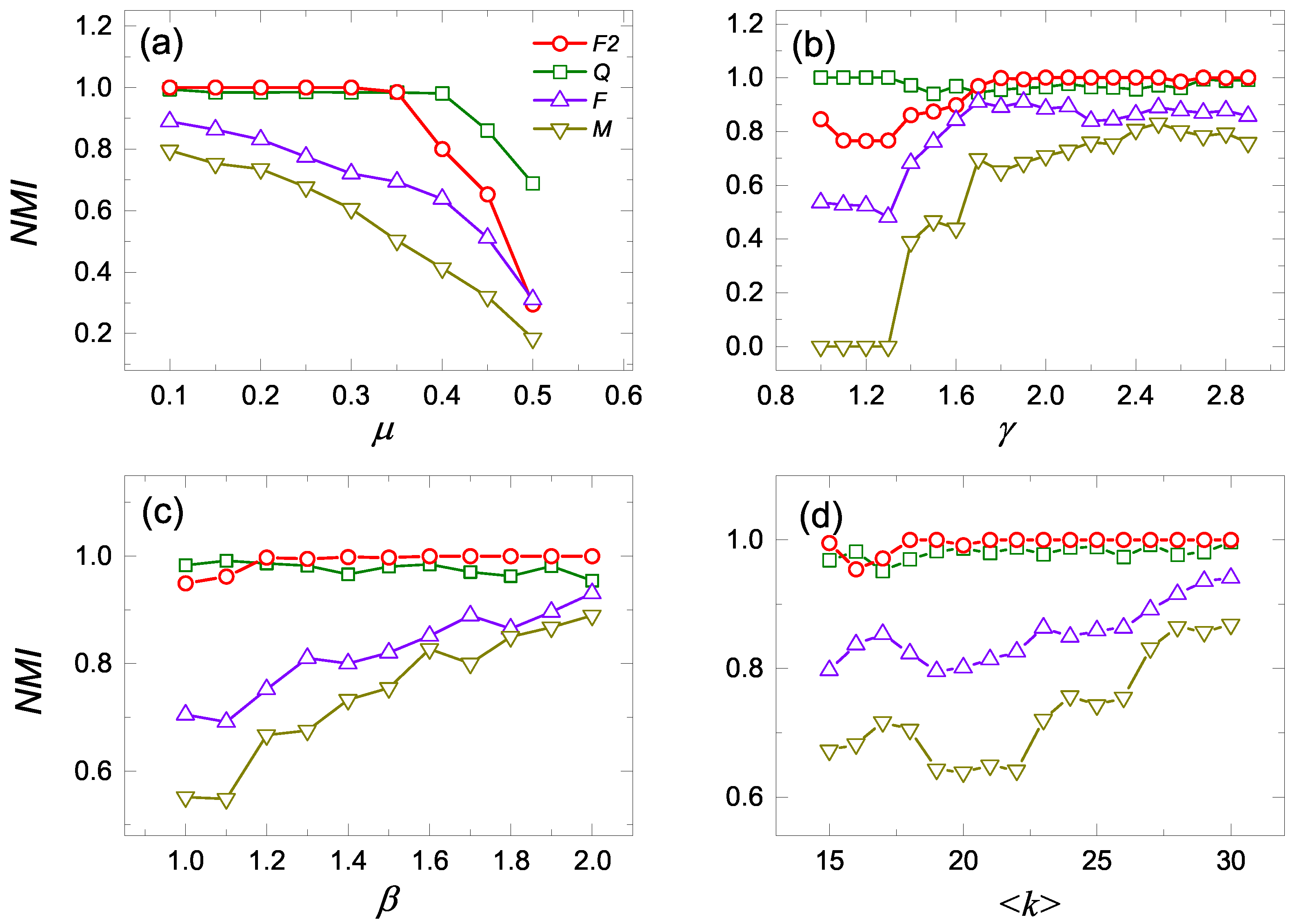
We also ran the constrained Louvain algorithm on the $LFR$ benchmark networks. In Figure 2a, the $NMI$ values of the constrained Louvain with $F2$ are highest when $\mu <0.4$. With the increase in $\mu$, the community structure becomes more fuzzy and harder to identify, all $NMI$ values decrease and the $NMI$ value of the constrained Louvain algorithm with $F2$ becomes less than the one with Q. This demonstrates that the constrained Louvain algorithm with $F2$ has the best performance for the networks with a clear community structure. Here, it is not necessary to calculate the cases of $\mu >0.5$, because the communities are not satisfying the definition of a weak community. In Figure 2b, for the small value of $\gamma$, the $NMI$ values of the constrained Louvain algorithm with Q are the highest. However, with the increase in $\gamma$, the heterogeneity of networks becomes stronger and the $NMI$ values of the constrained Louvain algorithm with $F2$ becomes higher than the constrained Louvain algorithm with other objective functions. Obviously, the stronger the heterogeneity of the networks are, the better is the performance of $F2$. In Figure 2c, for the high values of the parameter $\beta$, the constrained Louvain algorithm with $F2$ has the highest $NMI$ values. 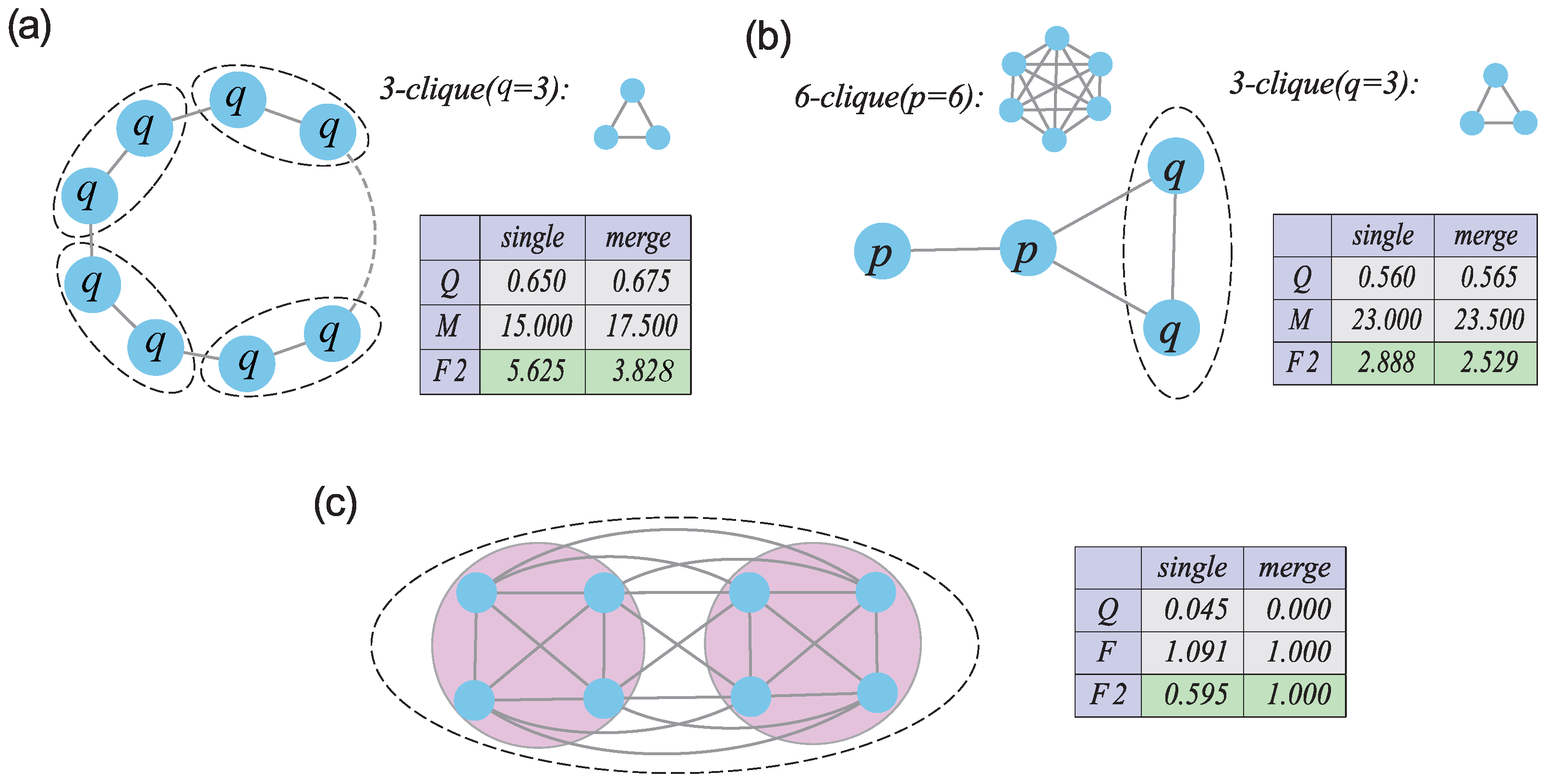With the increase in $\beta$ value, the distribution of the community sizes becomes heterogeneous so that the resolution limit problem appears for some objective functions. Due to the advantage of $F2$ in Figure 1, the constrained Louvain algorithm with $F2$ identifies the number of communities more correctly. In Figure 2d, the values of the $NMI$ are highest for the constrained Louvain algorithm with $F2$, regardless of the values of $\langle k\rangle$. In this case, the constrained Louvain algorithm with Q still has the resolution limit problem due to the small number of communities found. Moreover, the constrained Louvain algorithm with F and M obtains too many communities that are not satisfying the definition of a weak community, or the sizes are less then 4. As a result, the constrained Louvain algorithm with $F2$ can better identify the community structure.

Due to the optimal performance of the constrained Louvain algorithm with $F2$, it is expected to be a competitive algorithm. Next, we compare it with the classical Louvain algorithm with $F2$ and the Newman’s fast algorithm [13] by $NMI$ on ground truth networks and $LFR$ benchmark networks.

Table 3. The $NMI$ values for the constrained Louvain algorithm with F2, Louvain algorithm with F2 and Newman fast algorithm on the ground truth networks. The / means the algorithm cannot be executed for the large networks.

Algorithms	Constrained Louvain Algorithm	Louvain Algorithm	Fast Algorithm
Karate	0.6021	0.6021	0.6925
Dolphins	1.000	0.6741	0.7026
Football	0.9114	0.9336	0.6977
DBLP	0.7566	0.7547	/
Amazon	0.9854	0.9542	/

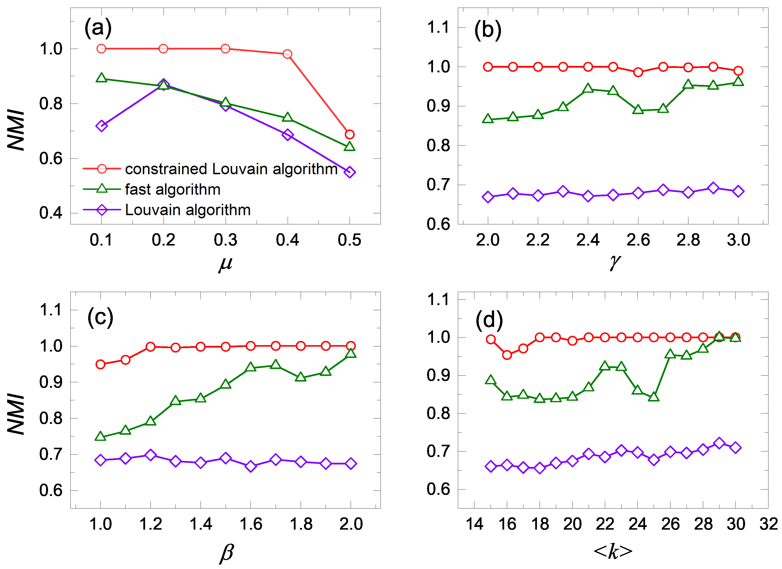
gives the values of $NMI$ on ground truth networks. Compared with the classical Louvain algorithm based on $F2$, the constrained Louvain algorithm based on $F2$ is better except for the football network. Compared with the fast algorithm, the constrained Louvain algorithm is better except for the karate network. Moreover, for the DBLP and Amazon networks, the cost of the fast algorithm is beyond our tolerance. In Figure 3, we also calculate the values of $NMI$ when one parameter is changed for parameters $\mu$, $\gamma$, $\beta$ and $\langle k\rangle$. As a result, the constrained Louvain algorithm with $F2$ has the highest values of $NMI$, which perform better than the other two methods. Therefore, the constrained Louvain algorithm with $F2$ can identify communities better.

5. Conclusions

The Louvain algorithm aims to optimize an objective function of the whole network, so it can excellently detect the community structure. Moreover, the Louvain method has a high efficiency. However, the communities obtained by the classical Louvain algorithm are not still the real communities. In this paper, we proposed a new local modularity function $F2$ as an objective function of optimization. $F2$ can overcome certain problems of other modularity functions such as the resolution limit problem and does not split the well-connected network into small communities. Both theoretical deductions and some examples suggest that $F2$ identifies communities better than the objective functions of $Q,F,M$. Thus, $F2$ is competitive as an objective function. Then, we proposed the constrained Louvain algorithm by adding the constraints $F2>0.25$, and the node number of each community is larger than 3 to the Louvain algorithm. This is because there exists some small communities and some communities that are not satisfying the weak community among the communities obtained by the Louvain algorithm. The constraints are meaningful. Finally, on both the real-world networks and the computer generated benchmark networks, the constrained Louvain algorithm with $F2$ shows a high accuracy of identifying community structures in most of the considered networks.

For hierarchical networks, we can add tunable parameters [48] in $F2$ to detect the hierarchical structure by the constrained Louvain algorithm. Through proper revisions, the constrained Louvain algorithm with $F2$ can be easily extended to directed or weighted networks. With the development of the computer technique, the data of the large network and dynamic network are more easily collected. Therefore, the community detection of dynamic and large networks is an interesting and challenging topic [49,50]. At the same time, the constrained Louvain algorithm can be paralleled, which is the same as the classical Louvain paralleled algorithm [30,31,51,52]. This is helpful for community detection in large or dynamic networks.

In the interdisciplinary area, the Louvain algorithm has many applications, such as disease modules’ identification [53], a hierarchical clustering approach of network embedding [54], the spatiotemporal analysis of a bike-share system [55] and the analysis of wireless sensor networks [56,57]. Our constrained Louvain algorithms are also applied to these fields. Moreover, modularity functions can be used to assess the training results for neural networks [58]. Our study on the modularity function $F2$ may hopefully lead to further studies that might be worth pursuing.

References

1. Albert, R.; Barabási, A.-L. Statistical mechanics of complex networks. Rev. Mod. Phys. 2002, 74, 47–97. [Google Scholar] [CrossRef] [Green Version]
2. Watts, D.J.; Strogatz, S.H. Collective dynamics of ‘small world’networks 1998. Nature 1998, 393, 440–442. [Google Scholar] [CrossRef] [PubMed]
3. Milgram, S. The small world problem. Psychol. Today 1967, 2, 60–67. [Google Scholar]
4. Barabási, A.-L.; Albert, R. Emergence of scaling in random networks. Science 1999, 286, 509–512. [Google Scholar] [CrossRef] [Green Version]
5. Barabási, A.-L.; Albert, R.; Jeong, H. Mean-field theory for scalefree random networks. Phys. A 1999, 272, 173–187. [Google Scholar] [CrossRef] [Green Version]
6. Girvan, M.; Newman, M.E.J. Community structure in social and biological networks. Proc. Natl. Acad. Sci. USA 2002, 99, 7821–7826. [Google Scholar] [CrossRef] [PubMed] [Green Version]
7. Newman, M.E.J. Detecting community structure in networks. Eur. Phys. J. B 2004, 38, 321–330. [Google Scholar] [CrossRef]
8. Flake, G.W.; Lawrence, S.; Lee, G.C.; Coetzee, F.M. Self-organization and identification of web communities. IEEE Comput. 2002, 35, 66–70. [Google Scholar] [CrossRef] [Green Version]
9. Krebs, V. Social Network Analysis Software & Services for Organizations, Communities, and their Consultants. Available online: http://www.orgnet.com (accessed on 1 January 2023).
10. Yang, J.; Leskovec, J. Defining and evaluating network communities based on ground-truth. In Proceedings of the 12th IEEE International Conferences on Data Mining (ICDM 2012), Brussels, Belgium, 10–13 December 2012; pp. 745–754. [Google Scholar]
11. Fortunato, S. Community detection in graphs. Phys. Rep. 2010, 486, 75–174. [Google Scholar] [CrossRef] [Green Version]
12. Radicchie, F.; Castellano, C.; Cecconi, F.; Loreto, V.; Parisi, D. Defining and identifying communities in networks. Proc. Natl. Acad. Sci. USA 2004, 101, 2658–2663. [Google Scholar] [CrossRef] [Green Version]
13. Newman, M.E.J. Fast algorithm for detecting community structure in networks. Phys. Rev. E 2004, 69, 066133. [Google Scholar] [CrossRef] [Green Version]
14. Xie, W.B.; Lee, Y.L.; Wang, C.; Chen, D.B.; Zhou, T. Hierarchical clustering supported by reciprocal nearest neighbors. Inf. Sci. 2020, 527, 279–292. [Google Scholar] [CrossRef] [Green Version]
15. Pan, Y.; Li, D.H.; Liu, J.G.; Liang, J.Z. Detecting community structure in complex networks via node similar. Phys. A 2010, 389, 2849–2857. [Google Scholar] [CrossRef]
16. Donetti, L.; Muñoz, M.A. Detecting network communities: A new systematic and efficient algorithm 2004. J. Stat. Mech. 2004, 2004, P10012. [Google Scholar] [CrossRef] [Green Version]
17. Capocci, A.; Servedio, V.D.P.; Caldarelli, G.; Colaiori, F. Detecting communities in large networks. Phys. A 2005, 352, 669–676. [Google Scholar] [CrossRef] [Green Version]
18. Jin, J. Fast community detection by SCORE. Ann. Stat. 2015, 43, 57–89. [Google Scholar] [CrossRef]
19. Zhou, H. Distance, dissimilarity index, and network community structure. Phys. Rev. E 2003, 67, 061901. [Google Scholar] [CrossRef] [PubMed] [Green Version]
20. Shao, J.; Han, Z.; Yang, Q.; Zhou, T. Community detection based on distance dynamics. In Proceedings of the 21th ACM SIGKDD International Conference on Knowledge Discovery and Data Mining, Sydney, NSW, Australia, 10–13 August 2015; pp. 1075–1084. [Google Scholar]
21. Hu, Y.; Chen, H.; Zhang, P.; Li, M.; Di, Z.; Fan, Y. Comparative definition of community and corresponding identifying algorithm. Phys. Rev. E 2008, 78, 026121. [Google Scholar] [CrossRef] [Green Version]
22. Rosvall, M.; Bergstrom, C.T. Maps of Random Walks on Complex Networks Reveal Community Structure. Proc. Natl. Acad. Sci. USA 2008, 105, 4. [Google Scholar] [CrossRef] [PubMed] [Green Version]
23. Raghavan, U.N.; Albert, R.; Kumara, S. Near linear time algorithm to detect community structures in large-scale networks. Phys. Rev. E 2007, 76, 036106. [Google Scholar] [CrossRef] [Green Version]
24. Chen, Y.; Zhou, L.; Pei, S.; Yu, Z.; Chen, Y.; Liu, X.; Du, J.; Xiong, N. KNN-BLOCK DBSCAN: Fast clustering for large-scale data. IEEE Trans. Syst. Man Cybern. Syst. 2019, 51, 3939–3953. [Google Scholar] [CrossRef]
25. Clauset, A.; Newman, M.E.J.; Moore, C. Finding community structure in very large networks. Phys. Rev. E 2004, 70, 066111. [Google Scholar] [CrossRef] [Green Version]
26. Blondel, V.D.; Guillaume, J.; Lambiotte, R.; Lefebvre, E. Fast unfolding of communities in large networks. J. Stat. Mech. 2008, 367, P10008. [Google Scholar] [CrossRef] [Green Version]
27. Zhu, J.; Ren, X.; Ma, P.; Gao, K.; Wang, B.-H.; Zhou, T. Detecting network communities via greedy expanding based on local superiority index. Phys. A 2022, 603, 127722. [Google Scholar] [CrossRef]
28. Newman, M.E.J.; Girvan, M. Finding and evaluating community structure in networks. Phys. Rev. E 2004, 69, 026113. [Google Scholar] [CrossRef] [PubMed] [Green Version]
29. Wu, Z.; Wang, P.; Qin, Z.; Jiang, S. 2013 Improved algorithm of Louvain communities dipartition. J. Univ. Electron. Sci. Technol. China 2013, 42, 105–108. [Google Scholar]
30. Mohammadi, M.; Fazlali, M.; Hosseinzadeh, M. 2021 Accelerating Louvain community detection algorithm on graphic processing unit. J. Supercomput. 2021, 77, 6056–6077. [Google Scholar] [CrossRef]
31. Mohammadi, M.; Fazlali, M.; Hosseinzadeh, M. Parallel Louvain Community Detection Algorithm Based on Dynamic Thread Assignment on Graphic Processing. Unit J. Electr. Comput. Eng. Innovations 2022, 10, 75–88. [Google Scholar]
32. Zhang, Z.; Pu, P.; Han, D.; Tang, M. Self-adaptive Louvain algorithm: Fast and stable community detection algorithm based on the principle of small probability event. Phys. A 2018, 506, 975–986. [Google Scholar] [CrossRef]
33. Zhang, J.; Fei, J.; Song, X.; Feng, J. An improved Louvain algorithm for community detection. Math. Probl. Eng. 2021, 2021, 1485592. [Google Scholar] [CrossRef]
34. Lancichinetti, A.; Fortunato, S.; Kertész, J. Detecting the overlapping and hierarchical community structure in complex networks. New J. Phys. 2009, 11, 033015. [Google Scholar] [CrossRef]
35. Luo, F.; Wang, J.Z.; Promislow, E. Exploring local community structures in large networks. In Proceedings of the IEEE/WIC/ACM International Conference on Web Intelligence, Hong Kong, China, 18–22 December 2006. [Google Scholar]
36. Fortunato, S.; Barthélemy, M. Resolution limit in community detection. Proc. Natl. Acad. Sci. USA 2007, 104, 36–41. [Google Scholar] [CrossRef] [Green Version]
37. Arenas, A.; Fernández, A.; Gómez, S. Analysis of the structure of complex networks at different resolution levels. New J. Phys. 2008, 10, 053039. [Google Scholar] [CrossRef] [Green Version]
38. Andrea, L.; Santo, F. Limits of modularity maximization in community detection. Phys. Rev. E 2011, 84, 066122. [Google Scholar]
39. Džamić, D.; Pei, J.; Marić, M.; Mladenović, N.; Pardalos, P.M. Exponential quality function for community detection in complex networks. Int. Trans. Oper. Res. 2020, 27, 245–266. [Google Scholar] [CrossRef] [Green Version]
40. Chen, M.; Nguyen, T.; Szymanski, B. A new metric for quality of network community structure 2013. ASE Hum. J. 2013, 2, 15. [Google Scholar]
41. Guimerà, R.; Sales-Pardo, M.; Amaral, L.A.N. Modularity from fluctuations in random graphs and complex networks. Phys. Rev. E 2004, 70, 025101. [Google Scholar] [CrossRef] [Green Version]
42. Reichardt, J.; Bornholdt, S. Statistical mechanics of community detection. Phys. Rev. E 2006, 74, 016110. [Google Scholar] [CrossRef] [Green Version]
43. Lancichinetti, A.; Fortunato, S.; Radicchi, F. Benchmark graphs for testing community detection algorithms. Phys. Rev. E 2008, 78, 046110. [Google Scholar] [CrossRef] [Green Version]
44. Zachary, W.W. An Information Flow Model for Conflict and Fission in Small Groups. J. Anthropol. Res. 1977, 33, 452–473. [Google Scholar] [CrossRef] [Green Version]
45. Lusseau, D.; Boisseau, O.J.; Slooten, E.; Dawson, S.M. The Bottlenose Dolphin Community of Doubtful Sound Features a Large Proportion of Long-Lasting Associations: Can Geographic Isolation Explain This Unique Trait? Behav. Ecol. Sociobiol. 2003, 54, 396–405. [Google Scholar] [CrossRef]
46. Lusseau, D.; Newman, M.E.J. Identifying the role that animals play in their social networks. Proc. R. Soc. Lond. Ser. B Biol. Sci. 2004, 271, S477–S481. [Google Scholar] [CrossRef] [Green Version]
47. Fred, A.L.N.; Jain, A.K. Robust data clustering. In Proceedings of the 2003 IEEE Computer Society Conference on Computer Vision and Pattern Recognition, Madison, WI, USA, 18–20 June 2003; Volume 128. [Google Scholar]
48. Gao, K.; Ren, X.; Zhou, L.; Zhu, J. Automatic Detection ofMultilevel Communities: Scalable, Selective and Resolution-Limit-Free. Appl. Sci. 2023, 13, 1774. [Google Scholar] [CrossRef]
49. Seifikar, M.; Farzi, S.; Barati, M. C-blondel: An efficient louvain-based dynamic community detection algorithm. IEEE Trans. Comput. Soc. Syst. 2020, 7, 308–318. [Google Scholar] [CrossRef]
50. Li, M.; Qin, J.; Jiang, T.; Pedrycz, W. Dynamic relationship network analysis based on louvain algorithm for large-scale group decision making. Int. J. Comput. Intell. Syst. 2021, 14, 1242–1255. [Google Scholar] [CrossRef]
51. Zeng, J.; Yu, H. A scalable distributed louvain algorithm for large-scale graph community detection. In Proceedings of the 2018 IEEE International Conference on Cluster Computing (CLUSTER), Belfast, UK, 10–13 September 2018; pp. 268–278. [Google Scholar]
52. Ghosh, S.; Halappanavar, M.; Tumeo, A.; Kalyanaraman, A.; Lu, H.; Chavarria-Miranda, D.; Khan, A.; Gebremedhin, A. Distributed Louvain algorithm for graph community detection. In Proceedings of the 2018 IEEE International Parallel and Distributed Processing Symposium (IPDPS) IEEE Computer Society, Vancouver, BC, Canada, 21–25 May 2018; pp. 885–895. [Google Scholar]
53. Perrin, D.; Zuccon, G. Module Identification Recursive module extraction using Louvain and PageRank. F1000Research 2018, 7, 1286. [Google Scholar] [CrossRef] [Green Version]
54. Bhowmick, A.K.; Meneni, K.; Danisch, M.; Guillaume, J.-L.; Mitra, B. LouvainNE: Hierarchical louvain method for high quality and scalable network embedding. In Proceedings of the WSDM ’20: Ae Airteenth ACM International Conference on Web Search and Data Mining ACM, Houston, TX, USA, 3–7 February 2020; pp. 43–51. [Google Scholar]
55. Song, J.; Zhang, L.; Qin, Z.; Ramli, M.A. A spatiotemporal dynamic analyses approach for dockless bike-share system. Comput. Environ. Urban Syst. 2021, 85, 101566. [Google Scholar] [CrossRef]
56. Yao, Y.; Xiong, N.; Park, J.H.; Ma, L.; Liu, J. Privacy-preserving max/min query in two-tiered wireless sensor networks. Comput. Math. Appl. 2013, 65, 1318–1325. [Google Scholar] [CrossRef]
57. Cheng, H.; Xie, Z.; SHi, Y.; Xiong, N. Multi-step data prediction in wireless sensor networks based on one-dimensional CNN and bidirectional LSTM. IEEE Access 2019, 7, 117883–117896. [Google Scholar] [CrossRef]
58. Watanabe, C.; Hiramatsu, K.; Kashino, K. Understanding Community Structure in Layered Neural Networks. Neurocomputing 2018, 367, 84–102. [Google Scholar] [CrossRef] [Green Version]
Figure 1. Performances of different objective functions on several representative networks. (a) Several 3-cliques connected to a ring through single edges (Reprinted/adapted with permission from Ref. [36], Copyright (2007) National Academy of Sciences, U.S.A.). On this network, two candidate community structures are generated. One is to identify each q-clique as a single community. The other is to merge each pair of adjacent cliques into one community. The values of modularity functions Q, M and F 2 for these two structures are listed as ‘single’ and ‘merge’ when the network contains 10 3-cliques in the inserted table. (b) A network consisting of two 6-cliques and two 3-cliques (reprinted/adapted with permission from Ref. [36], Copyright (2007) National Academy of Sciences, U.S.A.). ‘Single’ in the inserted table refers to identifying each clique as an individual community, while ‘merge’ refers to the integration of the two 3-cliques. (c) A well-connected network which is more compact than networks of Figure 1 in Ref. [40]. “single” splits the network into two communities, while “merge” identifies the whole network as one community.
Applsci 13 04045 g001
Figure 2. For the L F R networks, the relationship between the values of NMI and the values of each parameter. (a) μ is changed when γ = 2.5 , β = 1.5 and k = 20 . (b) γ is changed when μ = 0.3 , β = 1.5 and k = 20 . (c) β is changed when μ = 0.3 , γ = 2.5 and k = 20 . (d) k is changed when μ = 0.3 , γ = 2.5 and β = 1.5 . The results are averaged for 100 networks with N = 1000 .
Applsci 13 04045 g002
Figure 3. The N M I values of the constrained Louvain algorithm with F 2 , the classical Louvain algorithm with F 2 and the Newman’s fast algorithm averaged on the 100 L F R networks with N = 1000 . (a) μ is changed when γ = 2.5 , β = 1.5 and k = 20 . (b) γ is changed when μ = 0.3 , β = 1.5 and k = 20 . (c) β is changed when μ = 0.3 , γ = 2.5 and k = 20 . (d) k is changed when μ = 0.3 , γ = 2.5 and β = 1.5 .
Applsci 13 04045 g003