Modeling and Analysis of Contactless Solar Evaporation for Scalable Application

Abstract

Zero-liquid discharge wastewater treatment driven by sunlight shows potential to minimize its environmental impact by producing solid-only waste from solar energy. To overcome the key barrier of solar absorber contamination, solar-driven contactless evaporation (SCE) has been proposed. However, only a small-scale laboratory device has been studied, which cannot support its scalable application. To analyze the potential of SCE, it is essential to understand the conjugated heat and mass transfer under a scalable application scenario. In this study, a comprehensive model of SCE is developed, which is validated by the laboratory evaporation test and applied to scalable evaporation scenario. Results showed that the scalable evaporation (0.313 kg·m⁻²·h⁻¹) could obtain higher evaporation rate than the laboratory evaporation (0.139 kg·m⁻²·h⁻¹) due to suppressed heat losses from the sidewalls. If the design parameters are finely tuned and thermal insulation are properly applied, the evaporation rate could be further enhanced to 0.797 kg·m⁻²·h⁻¹, indicating a 473.3% performance enhancement than the laboratory SCE. The modelling framework and understanding are expected to pave a way for the further improvement and scalable application of SCE.

1. Introduction

Two-thirds of the global population is affected by water shortage which has become a major global risk for human beings [1]. According to the World Economic Forum, water crises are mainly caused by the depletion of natural fresh water resources by agriculture, industry and urban use, as well as an ever-growing amount of wastewater [2]. Except for different wastewater produced from municipal and industrial processes, the freshwater supply technology itself could produce a huge amount of hypersaline wastewater. For instance, desalination of seawater [3,4,5,6] or brackish water [7] produces concentrated brine as an undesirable by-product. Conventional strategies for concentrated brine disposal include surface water discharge, deep well injection, evaporation ponds and land application [8], which are improper for wastewater treatment and detrimental to soil, land vegetation and the aquatic ecosystem [9,10,11,12].

Zero-liquid discharge (ZLD), a wastewater management strategy that can completely separate salt from water with minimized impact to the aquatic environment, has attracted worldwide interests [7,12,13]. Currently, the ZLD wastewater treatment is mainly divided into two stages [7]. First, the wastewater is concentrated by either membrane or thermal methods. Then, the concentrated brine is turned into solid waste by using an evaporation pond or crystallizer [14]. With a sophisticated mechanical structure, the crystallizer has a smaller footprint, but it is highly energy intensive (>50 kWh·m⁻³) and produces large amounts of carbon emissions [14,15]. On the contrary, the evaporation pond harvests solar energy to evaporate the water in concentrated brine, which has lower carbon emissions and operating costs. However, it has a low evaporation efficiency and large footprint (>1000 m⁻²), due to the low energy density of sunlight [16,17]. In order to improve the competitiveness of this low-carbon technology, it is critical to enhance the energy efficiency of solar evaporation ponds [18,19,20].

In recent years, solar-driven interfacial evaporation has been intensively investigated, due to its great potential to achieve high-efficiency desalination and wastewater treatment [6,21,22,23,24,25]. The porous evaporator with low thermal conductivity localizes the solar thermal energy at the air–liquid interface to achieve high solar evaporation efficiency. However, the porous evaporator also constrains the salt transport, resulting in fast salt accumulation and crystallization. The salt crystallization will reduce the light absorption and water supply, resulting in a low evaporation rate or even complete evaporation failure [26,27,28,29]. To overcome the salt accumulation issues, different strategies have been proposed, including salt diffusion enhancement [30,31,32], salt crystals rinsing [33], multi-layer design [34], and other strategies. Nevertheless, the salt crystallization problem cannot be completely solved as the solar absorber and air–water interface are still in contact.

To totally eliminate the salt crystallization on the solar absorber, solar-driven contactless evaporation (SCE) was proposed by Cooper et al. [35], as shown in Figure 1. In this design, the solar energy is converted into thermal energy by the solar absorber, and then emitted in the form of infrared thermal radiation. The infrared radiation can be efficiently absorbed by water within a thin layer (~10 μm) due to the high absorptivity of water [36]. The contactless design archives interfacial heating via radiative heat transfer, which can thoroughly prevent salt accumulation and fouling issues. Due to the application of high-temperature steam generation, the evaporation rate was lower than 0.39 kg·m⁻²·h⁻¹. Later, Prasher et al. investigated solar-driven contactless heating to enhance the evaporation performance of solar pond [37]. Due to the lower working temperature and multiple vapor escaping holes, the evaporation rate was increased to 0.62 kg·m⁻²·h⁻¹.

Despite the efforts in developing SCE, the performance was only analyzed with a small-scale laboratory device where the wastewater pond was simulated with a small container (35 mm × 35 mm × 50 mm). The performance potentials of the scaled-up SCE device are still unclear as there are several factors which need deeper investigations. First, the coupled heat and mass transfer in a scalable solar evaporation device may vary significantly from that of the laboratory test rig. For instance, boundary conditions in both air and water domains are different [37,38]. Second, the previous laboratory study overlooked the impact of the configurations and designs of vapor escaping holes. Further parametric investigations on structural design are needed for evaluating the performance potentials of the scalable device. In this study, a detailed numerical modelling framework of the SCE process is developed to study the conjugated heat and mass transfer mechanism in the evaporation and transport processes and to reveal influential factors for optimizing the evaporation rate. The modelling framework is validated by lab-scale experiments and applied to the scalable solar evaporation scenario, through boundary condition variations. Results show that the evaporation rate of scalable SCE (0.313 kg·m⁻²·h⁻¹) is much higher than that of the laboratory evaporation with a container (0.139 kg·m⁻²·h⁻¹). Through parametric optimization and energy flow analysis, two major heat-loss mechanisms can be identified, including the heat conduction through the water bottom (16.2% of the total energy input) and heat convection on the solar absorber surface occupy (36.8% of the total energy input). Therefore, thermal insulation for heated water and solar absorber can effectively reduce the heat loss. With proper design and thermal insulation, the evaporation rate of scalable SCE could be further enhanced to 0.797 kg·m⁻²·h⁻¹, indicating a 473.3% performance enhancement potential than the laboratory SCE. The energy conversion efficiency is 50.3%, which is the highest one in the SCE process.

2. Methodology

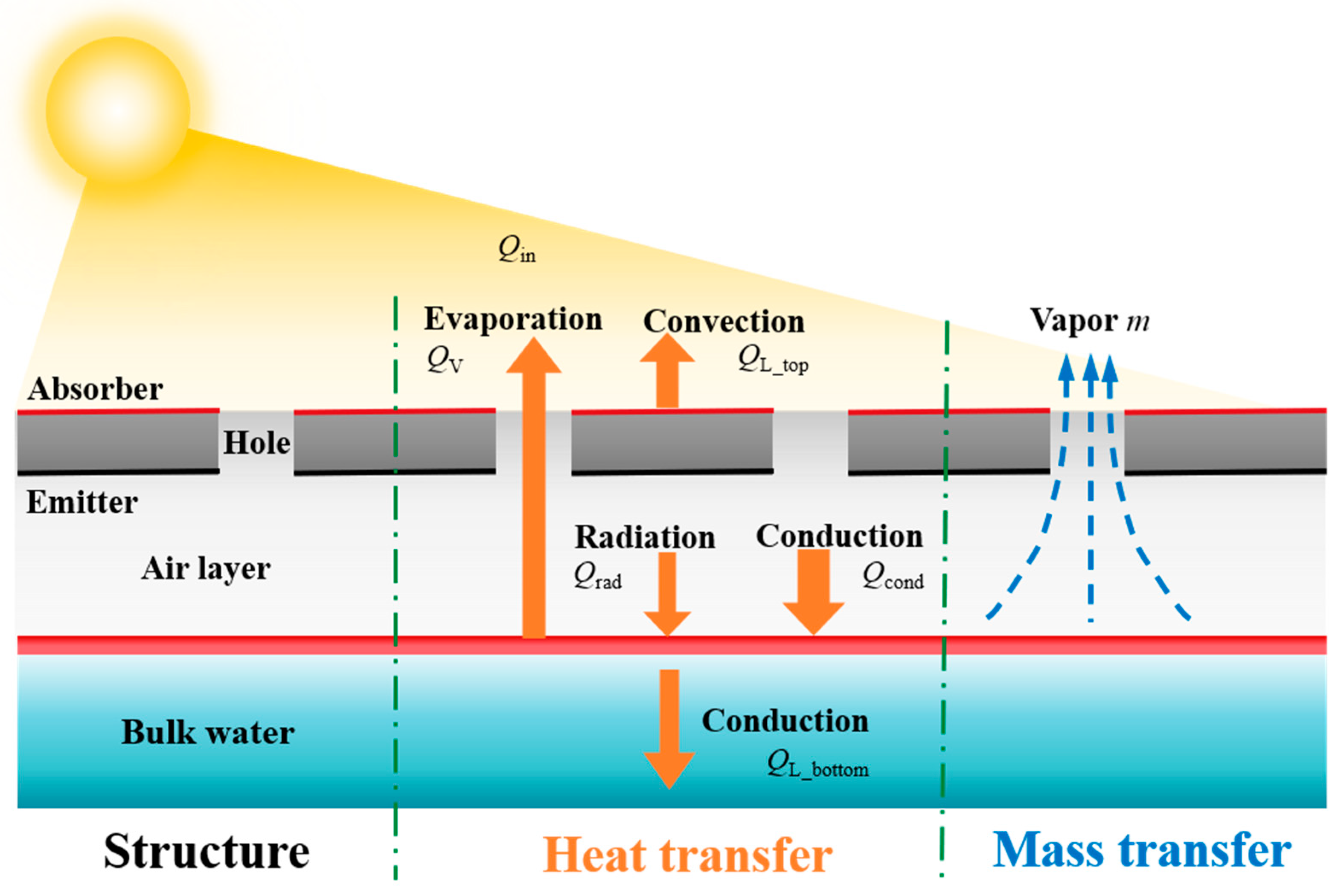
2.1. Working Principle

To study the heat and mass transfer of SCE in both laboratory and scalable application scenarios, two 3D models in COMSOL Multiphysics are built. The model for laboratory device is built according to the SCE device in the previous literature [37], including aluminum foil, absorber–emitter, insulation foam, bulk water and a container wall, as shown in Figure 2a. The absorber–emitter is the key energy conversion component in this device, which absorbs the sunlight on top and emits infrared thermal radiation on bottom. The infrared thermal radiation will further be absorbed by the water in the container. To create the air gap separating the water and the absorber–emitter, the absorber–emitter is set on top of the container wall, while the water level is lower than the container wall. To avoid the extra solar heating of container wall, a thin layer of aluminum foil is covered on top of the container wall, surrounding the square absorber–emitter. To reduce the heat loss from the absorber–emitter to the ambient environment, thermally-insulated foam is set beneath the aluminum foil. The model for a scalable device is built according to its application on solar evaporation pond with large surface area, without aluminum foil, insulation foam and walls, as shown in Figure 2b. The absorber–emitter used in both models are considered as a copper plate with selective absorption coating on top and emittance-enhancing coating on bottom, as shown in Figure 2c. This is also consistent with the previous literature [35,37]. Straight holes are equidistantly drilled on the absorber–emitter for vapor escaping. In both devices, solar energy is absorbed by the absorber–emitter to heat up the water near air–water interface. The water vapor generated will then escape from the holes on absorber–emitter. However, heat losses will also exist from absorber–emitter and water to the ambient. In general, the two models share the same working principle. In this case, the effectiveness of both models could be ensured, if one model is validated.

The detailed geometrical parameters of the laboratory and scalable devices are listed in

Table 1. Geometrical parameters of the laboratory and scalable devices.

Parts	Dimension
	Laboratory Device	Scalable Device
Absorber–emitter [A × B × C]	35 mm × 35 mm × 1.5 mm	11.67 mm × 11.67 mm × 1.5 mm
Bulk water [A × B × C]	35 mm × 35 mm × 50 mm	11.67 mm × 11.67 mm × 50 mm
Container side wall thickness	20 mm	None
Container bottom wall thickness	20 mm	20 mm
Air gap thickness	2 mm	2 mm
Number of straight holes	9	1
Thickness of the insulation foam	3.5 mm	None

. The size of the absorber–emitter in the laboratory device was set as 35 mm, 35 mm, 1.5 mm for depth, width and height, respectively, determined by the experiment setup. The straight holes distribution of laboratory device was set as 3 × 3. Since the scalable model is to study the conjugate heat and mass transfer in a single hole for scalable application scenarios, its geometric structure was scaled down equally according to the laboratory device, with A, B and C of 11.67 mm, 11.67 mm, 1.5 mm, respectively.

2.2. Modelling Framework

Based on the working principles of two devices shown above, the modelling framework considered the heat transfer, fluid flow and moisture transport, resulting in a complex multiple-physical process. Initially, as shown in Figure 1, solar energy is absorbed by the absorber–emitter as the input energy (Q_in), which heats up the water near the air–water interface through radiation (Q_rad) and conduction (Q_cond). Meanwhile, there exists the top heat loss (Q_{L_top}) through the absorber surface to the environment. The latent heat (Q_v) of evaporation carries the energy, which is delivered to the vapor through phase change at the air–water interface. The mass flux (m) associated with the heat flux enters the air layer simultaneously, leading to a continuous vapor generation, which then escapes from the holes on the absorber–emitter. There also exists the bottom heat loss (Q_{L_bottom}) through the bulk water to the environment. The following assumptions were applied in this study:

(1)

The moist air is in saturated state (RH = 100%) on the water surface;

(2)

In the scalable model, the view factor is set to 1 between the infrared emitter surface and the water surface;

(3)

Both in laboratory and scalable models, the bulk water is set as solid domain.

To capture the heat transfer in both solid and fluid domains, governing equations shown in Equations (1) and (2) were applied for water, air, thermally insulated foam and container walls.

$$\rho C_{p}u\cdot \nabla T+\nabla q=Q_{\mathrm{h}}$$

(1)

$$q=-k\nabla T$$

(2)

where, ρ, C_p and u denote the density, heat capacity at constant pressure and velocity vector, respectively. q, and Q_h represent the conductive heat flux vector and the heat source, respectively. k and T are thermal conductivity and temperature.

To describe the flow in air domain, governing equations for laminar flow were adopted as shown in Equations (3) and (4), considering the slow movement.

$$\rho (u\cdot \nabla )u=\nabla \cdot [-pI+K]+F+\rho g$$

(3)

$$\nabla \cdot (\rho u)=0$$

(4)

where, I, K and F represent identity matrix, the shear tensor, and the volume force vector, respectively. $g$ is the gravity acceleration.

To capture the vapor transport in air domain, governing equations shown in Equations (5)–(7) were adopted for moisture transport in air.

$$M_{v}u\cdot \nabla c_v+\nabla \cdot g=G$$

(5)

$$g=-M_{v}D\nabla c_v$$

(6)

$$c_v=\phi c_{\mathrm{sat}}$$

(7)

where, M_v, c_v, $g$, and G represent the molar mass of water vapor, water vapor concentration, diffusion flux of vapor and the moisture source, respectively. D is the vapor diffusion coefficient in air. φ and c_sat are the relative humidity (RH) and the vapor saturation concentration, respectively.

The heat transfer and mass transfer were coupled through Eqs. 8 and 9, the flow and heat transfer are coupled through Equations (10) and (11).

$$q_{\mathrm{evap}}=-L_v{g}_{\mathrm{evap}}$$

(8)

$$Q_p={\alpha }_{p}T(\frac{\partial p}{\partial t}+u\cdot \nabla p)$$

(9)

$${\alpha }_p=-\frac{1}{\rho }{(\frac{\partial \rho }{\partial T})}_p$$

(10)

$$Q_{\mathrm{vd}}=\tau :\nabla u$$

(11)

where q_evap, L_v and g_evap are the phase change heat flux, latent heat of evaporation and evaporative vapor flux, respectively. ${\alpha }_p$ and $\tau$ are the coefficient of thermal expansion and the viscous stress tensor.

To solve the multiple-physical fields coupling problem, the laboratory SCE model applied the following boundary conditions: a constant heat flux (Q_in one-sun solar radiation) boundary on the solar absorber surfacer. The radiative heat transfer process of infrared emitter and water surface is represented by setting boundary heat sources based on Stefan–Boltzmann law on the infrared emitter and water surface, respectively. The expressions of boundary heat sources are shown in Equations (12) and (13). Convective heat flux boundary was applied on the sidewall of laboratory SCE, considering a constant ambient temperature of 25 ℃. The open boundaries were applied on the outer boundaries of the air domain.

$$Q_{\mathrm{rad}-\mathrm{e}}=-F\epsilon \sigma (T_{\mathrm{e}}{}^4-T_{\mathrm{wat}-\mathrm{t}}{}^4)$$

(12)

$$Q_{\mathrm{rad}-\mathrm{wat}}=F\epsilon \sigma (T_{\mathrm{e}}{}^4-T_{\mathrm{wat}-\mathrm{t}}{}^4)(1-\phi )$$

(13)

where F, ε and σ represent the view factor_, emittance and Stefan–Boltzmann constant, respectively. T_e and T_wat are the temperature of emitter and water surface. φ is the hole area ratio.

As shown in Equation (14), the convective heat flux boundary in laboratory SCE was then replaced by periodic boundary conditions on the lateral surfaces in the scalable SCE, to simulate the large-scale application, whereas the rest settings were consistent in both SCE models.

$$\Delta T=0$$

(14)

The stable evaporation rate is the primary metric used to assess the performance of SCE system. Hence, the above modelling framework were solved in COMSOL Multiphysics with a stationary solver. The relative tolerance is 1e⁻³ considering both computational cost and accuracy. The material properties including thermal conductivity were also called from the COMSOL material library. The main input parameters for the two models are shown in

Table 2. Input parameters for the 3D COMSOL Multiphysics models.

Parameter	Value	Parameter	Value
Twat (°C)	25	${\alpha }_a$ (%)	96.32
Tae (°C)	25	${\epsilon }_e$ (%)	78.20
Tamb (°C)	25	${\epsilon }_{wall}$ (%)	95
${\phi }_{amb}$ (%)	50	hfg (kJ kg−1)	2500 − 2.386 × (T-273)
${\phi }_{\mathrm{wat}}$ (%)	100	D (m2 s−1)	1.87 × 10−10 (T/K)2.072/(P/atm)

.

Evaporation rates under different mesh configurations were studied to ensure mesh-independent results, and the results for scalable SCE model is shown in Figure 3. After increasing the element number from M₅ (455724) to M₆ (1778605), the difference in evaporation rate is less than 1%, indicating a mesh-independent result. The same method was also applied to the laboratory SCE model. With these analyses, the element numbers of 455724 and 2185976 were confirmed for the scalable and laboratory SCE models, respectively.

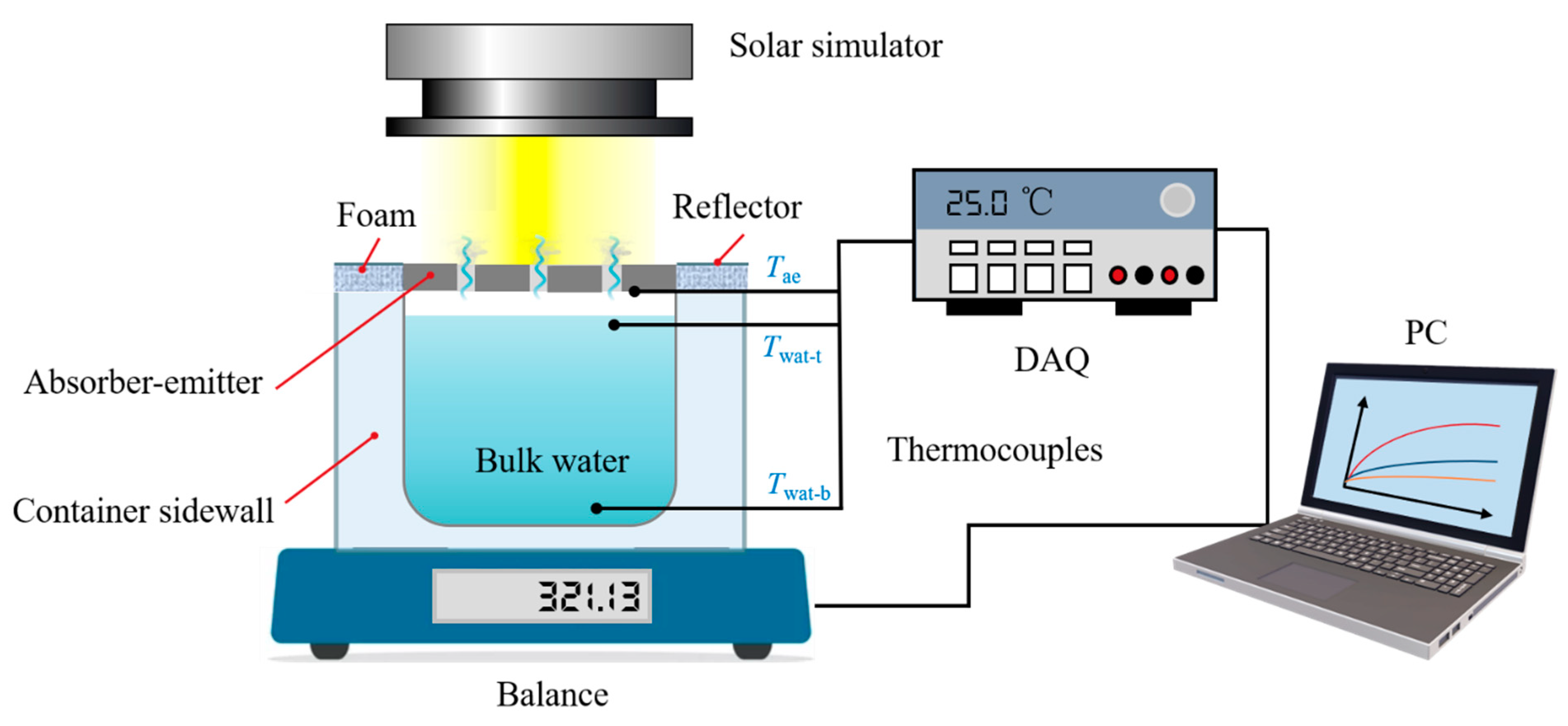
2.3. Experimental Setup

To verify the effectiveness of the proposed modelling framework, a laboratory SCE device was fabricated, tested and compared with the modelling results. Test rigs of the laboratory device are represented in Figure 4, containing a solar simulator, the foam topped with a reflector, an absorber–emitter, a container with pure water, a balance, three thermocouples, a data acquisition unit and a PC. The absorber–emitter was prepared as follows: Firstly, the copper plate was drilled uniformly and then polished and etched to achieve high absorptance of sunlight. Then, the emitter side was sprayed with black paint (Zynolyte Hi-Temp Paint; Aervoe) to achieve a high-emissivity paint. The solar simulator (Sciencetech, UHE-NS-100) was fixed and provided with a stable solar flux of 1000 W·m⁻². Three thermocouples were placed at the top surface (T_wat-t) and bottom surface (T_wat-b) of the bulk water, and the bottom surface of the absorber–emitter (T_ae) for measurement of temperatures. A weighing balance (Sartorius, GL22021—1SCN) was used to assess the change in mass of water as a proxy for evaporation rates. The data acquisition unit (Toprie, TP700) logged the signals from measuring instruments and monitored the readings.

3. Result and Discussion

With the modelling framework and experimental setup shown above, model validation and simulation analysis were carried out. First, the modelling framework was validated against the experiment data. Then, the comparative study of the laboratory, and the scalable SCE were completed. Second, the parametric analysis of the scalable SCE was carried out. Finally, the technical potential was explored based on the energy flow analysis of the scalable SCE.

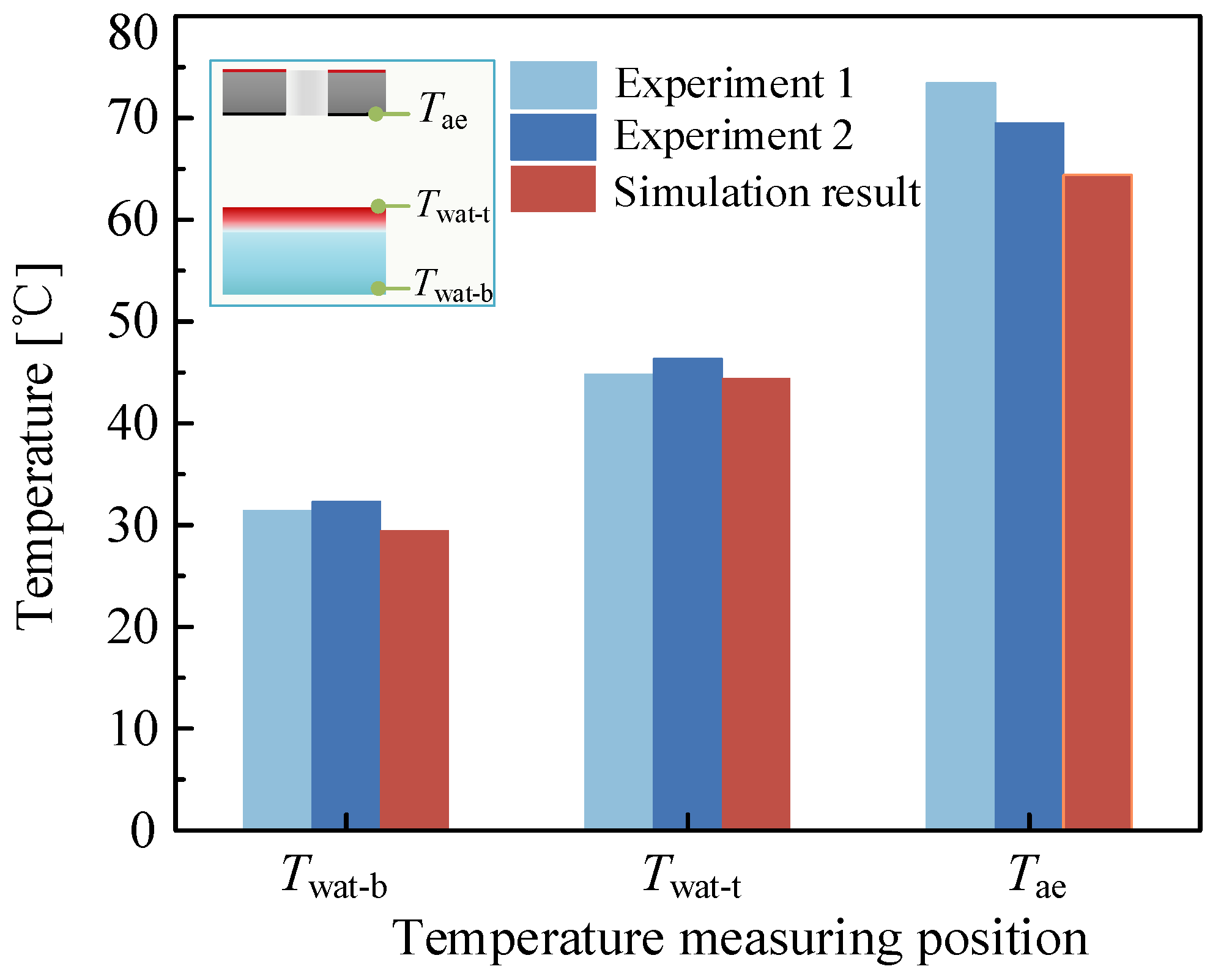
3.1. Modelling Validation

To verify the accuracy of the modelling framework, the simulation results were compared with the experimental results. Two repeated experiments using the test rig shown in Figure 4 were carried out, and the SCE models were solved under the same conditions shown in Table 2. As shown in Figure 5, three steady-state temperatures (T_wat-b, T_wat-t and T_ae) were obtained after 40 min from the start of the experiment, which exhibit small difference with the simulation results. The maximum error is less than 5%, indicating the mathematical models and boundary conditions applied to the laboratory SCE is effective. Since the scalable and laboratory SCE models only have differences in the boundary conditions on lateral surfaces, the rationality of the scalable SCE could also be ensured.

3.2. Comparison between the Laboratory and Scalable SCE

The size of the laboratory SCE device is limited by the solar simulator, which cannot describe the real operation of SCE with much larger size well. To analyze the difference between laboratory SCE and scalable SCE, a simulation-based analysis SCE for both scenarios was performed, as shown in Figure 6. Since the distribution of vapor escaping holes will be important in scalable application of SCE, the hole area ratio was also adjusted during the analysis. Figure 6 shows the evaporation rates of the two evaporators under hole area ratios of 0.7%, 14.4% and 36.9%, considering hole diameters of 1.1 mm, 5 mm and 8 mm, respectively. Evaporation rates of the laboratory SCE are 0.018 kg·m⁻²·h⁻¹, 0.139 kg·m⁻²·h⁻¹ and 0.205 kg·m⁻²·h⁻¹, respectively, whereas they are 0.067 kg·m⁻²·h⁻¹, 0.313 kg·m⁻²·h⁻¹ and 0.319 kg·m⁻²·h⁻¹ for the scalable SCE. It was found that the evaporation rate increases quickly with the hole area ratio, for both the laboratory and scalable SCE. More notably, the evaporation rates of the scalable SCE were much higher than that of the laboratory SCE under different hole area ratios.

To gain deeper insights into the evaporation rate difference between laboratory and scalable SCE, the heat balance of both two SCE processes were analyzed. Figure 6b shows the distribution of energy for both the laboratory and scalable SCE processes, under a hole area ratio of 14.4%. The heat loss of SCE could mainly be classified into the heat loss from water, heat loss from absorber–emitter and other heat loss (the radiation heat loss from the absorber surface to the environment and the convective heat loss between the vapor and the absorber–emitter). The first heat loss mechanism could further be classified into the sidewall loss and bottom loss. According to the analysis, 30.8% of total energy input is dissipated to the ambient through the sidewalls of laboratory SCE, which does not exist in scalable SCE. However, a large percentage of thermal energy is lost to the bottom water in the scalable SCE (31.9%), whereas this is only 8.8% for the laboratory SCE due to the large thermal resistance of bottom wall. Due to the stronger heat loss through sidewalls, the total heat loss from water is more severe for the laboratory SCE. The second heat loss mechanism is affected by both the heat loss area and temperature difference with the ambient. Although the scalable SCE has a higher temperature than its counterpart, it also has less heat loss area, since there is no extra sidewall supporting the absorber–emitter. In this case, the scalable SCE has 33.8% heat loss from absorber–emitter, which is slightly lower than the 36.8% for laboratory SCE. Both aspects explain the much lower evaporation rate of the laboratory SCE. The huge difference between laboratory and scalable SCE processes also validates our previous analysis that the experimental test cannot accurately explain the heat and mass transfer mechanisms of SCE in real, large-scale applications.

3.3. Parametric Analysis of the Scalable SCE

As the difference between laboratory and scalable SCE processes is identified, it is essential to further analyze the influences of different parameters on the SCE performance, under the scalable application scenario. This could be started from the conjugated heat transfer and vapor diffusion between the absorber–emitter and air-liquid interface, which directly decides the evaporation performance. This is further affected by the hole area ratio, hole diameter and air layer thickness, which have not been considered by previous studies. Figure 7 shows the heat and mass transfer affected by the absorber–emitter parameters, where the red and blue arrows represent the solar irradiation and vapor diffusion, respectively. The thermal energy received by the water surface decreases with a higher hole area ratio. The vapor diffusion is classified by two subsequent processes: horizontal diffusion towards the hole and vertical diffusion out of the hole. The horizontal diffusion is mainly affected by the center distance between adjacent hole, which is further decided by the hole number and hole area ratio. The vertical diffusion is mainly affected by the hole diameter, since a larger hole diameter provides lower diffusion resistance. There exists a clear conflict between the heat and mass transfer, making the parametric analysis necessary. Hence, the evaporation rate affected by the above three parameters are analyzed, considering the scalable SCE.

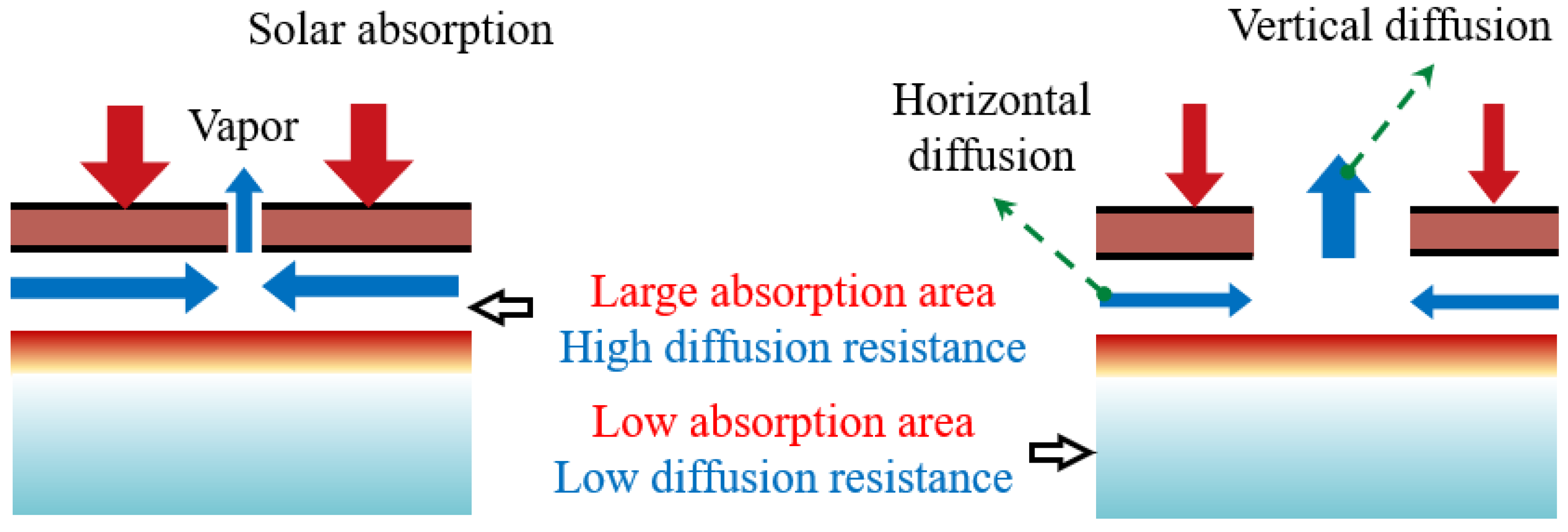
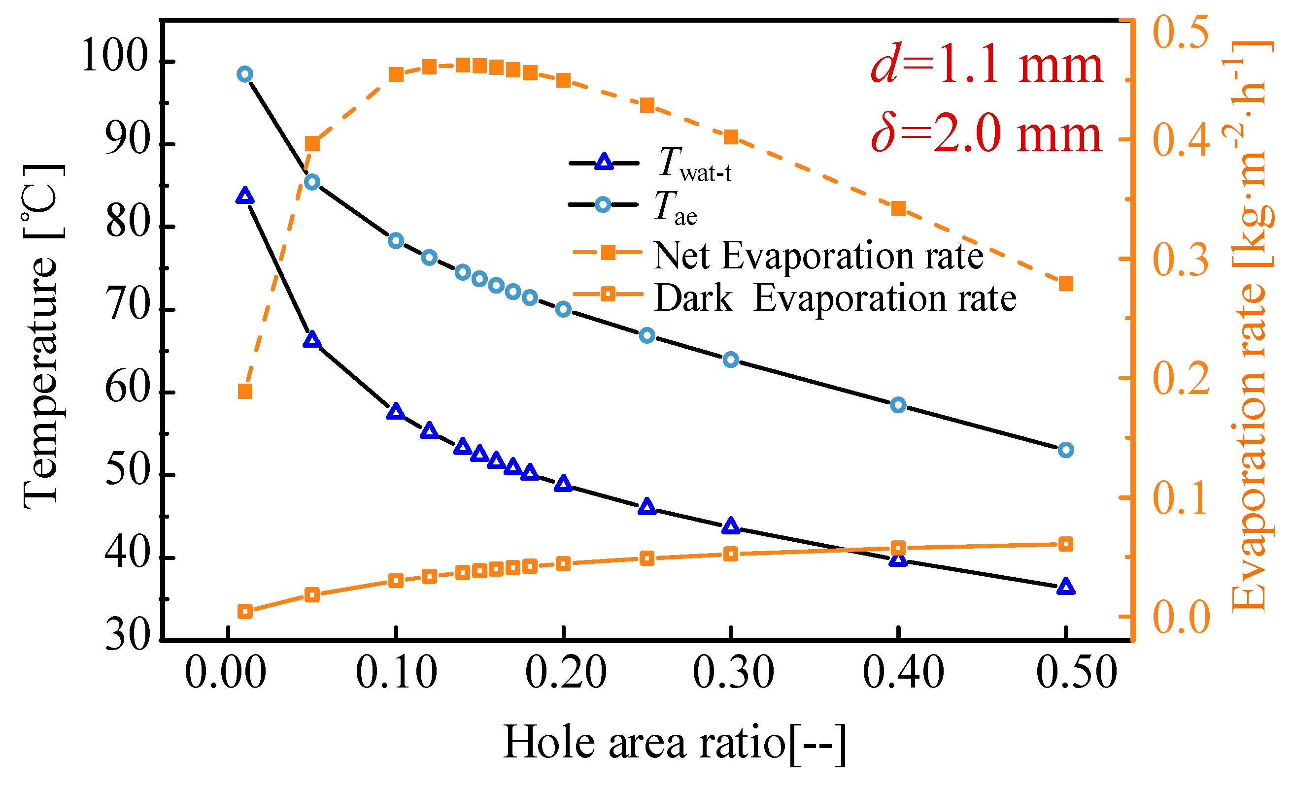
3.3.1. Hole Area Ratio

Figure 8 shows the absorber–emitter temperature T_ae, water surface temperature T_wat-t and evaporation rate under different hole area ratios, with the same hole diameter (d = 1.1 mm) and air layer thickness (δ = 2.0 mm). When the hole area ratio increases, both T_ae and T_wat-t decrease, due to less energy input from smaller absorber area. On the contrary, the natural evaporation rate under no solar input increases slightly (also referred as “dark evaporation” in the literature, which is decided purely by the vapor diffusion from water surface to the faraway ambient) due to the enhanced vapor diffusion with a larger diffusion area. The net contribution of solar input (referred as “net evaporation rate”) firstly increases, and then declines after the peak value of 0.463 kg·m⁻²·h⁻¹ is achieved under a hole area ratio of 14%. This can be explained by the conflict between increased solar absorption and enhanced vapor diffusion, whereas the overall impact to evaporation performance is decided by the relative significant of two aspects. When the hole area ratio is lower than 14%, the vapor diffusion enhancement is more important than the increased solar absorption, so the evaporation rate increases with a higher hole area ratio. When the hole area ratio is higher than 14%, the relative importance between vapor diffusion enhancement and increased solar absorption overturns, and the evaporation rate decreases with the higher hole area ratio. The above analyses indicates that an optimal hole area ratio exists (14%) to maximize the evaporation rate of scalable SCE. It is necessary to be noted that the optimal hole area ratio is dependent on the geometrical parameters and operation conditions.

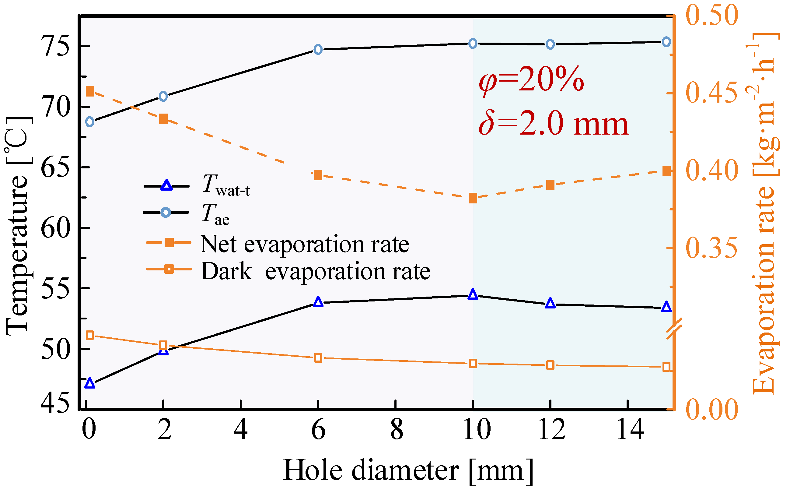
3.3.2. Hole Diameter

To further explore the effect of the hole diameter on the scalable SCE performance, the absorber–emitter temperature T_ae, water surface temperature T_wat-t and evaporation rate under different hole diameters, with the same hole area ratio (φ = 20%) and air layer thickness (δ = 2.0 mm) were obtained as shown in Figure 9. When the hole diameter increases, the dark evaporation rate increases, due to the enhanced vapor diffusion with lager vertical diffusion. At the same time, the net evaporation rate decreases firstly and then increase slightly after the low point of 0.412 kg·m⁻²·h⁻¹ is achieved under hole diameter of 10 mm, due to the conflict between the vertical and horizontal diffusion. On the contrary, both T_ae and T_wat-t increase firstly and then decrease slightly, due to the same energy input and different latent heat of evaporation. From the above analysis, it can be deduced that the effect of vertical diffusion on the scalable SCE performance is more important than that of horizontal diffusion. Hence, the selection of the hole diameter should be fully considered in real large-scale applications.

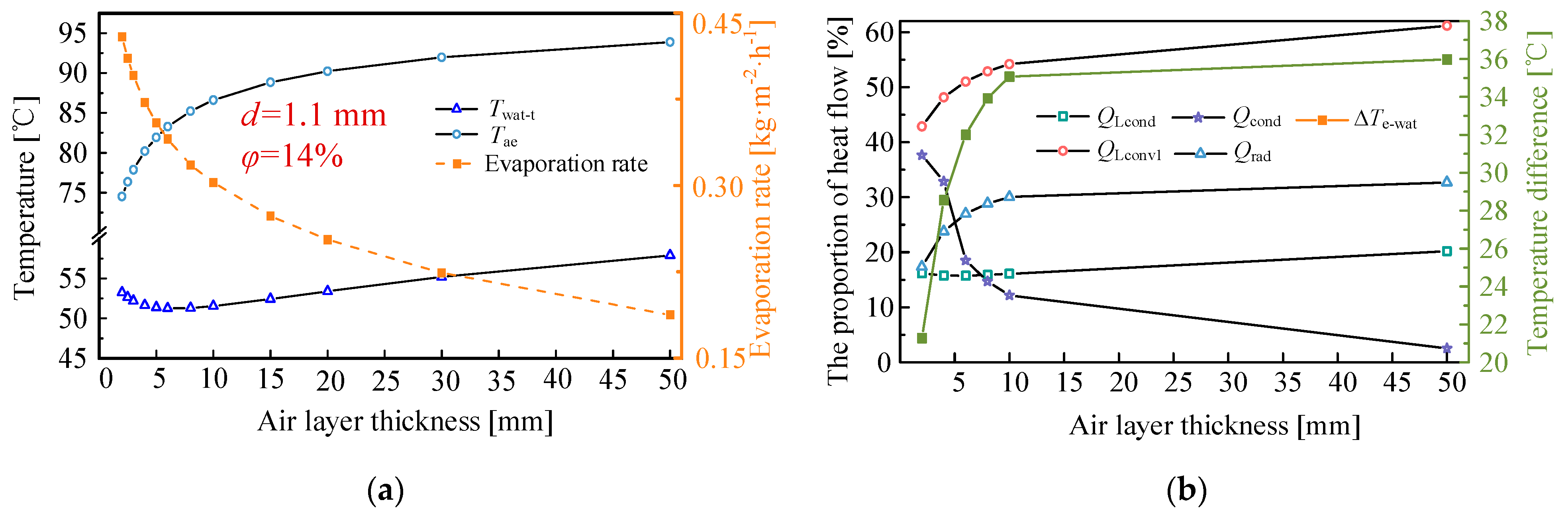
3.3.3. Air Layer Thickness

Besides the above two parameters, the distance between the bulk water surface and the emitter surface (referred as “air layer thickness”), which is also an important geometrical parameter for scalable SCE evaporation. This can be explained by the both variations of heat and mass transfer, due to the change in the resistance of heat transfer and the vapor diffusion, respectively.

Figure 10a shows the absorber–emitter temperature T_ae, water surface temperature T_wat-t and evaporation rate under different air layer thicknesses, with the same hole diameter (d = 1.1 mm) and hole area ratio (φ = 14%). When the air layer thickness increases, the evaporation rate decreases, due to the increased thermal conductivity resistance and weakened vapor diffusion. It is worth noting that the temperature difference between T_ae and T_wat-t increases firstly and then shows dynamic stability after the inflection point of 35.9 ℃ is achieved under the air layer thickness of 10 mm, as shown in Figure 10b. It can be explained that the temperature difference mainly depends on both the heat conduction flux and heat resistance in the air layer, when the air layer increases, the heat conduction resistance of air layer increases, while the proportion of the heat conduction flux decreases. Hence, when they tend to be in dynamic equilibrium, the temperature difference between the two remains constant at last. It can be highlighted that a thinner air layer above the water surface can improve evaporation performance because it reduces the distance that the evaporated molecules must travel before they are released into the atmosphere. This can lead to more efficient evaporation and a higher rate of mass transfer from the liquid to the gas phase.

3.4. Heat Loss Suppression for Scalable SCE

Although the key parameters of the SCE device have been analyzed and optimized, the evaporation rate is still at a relatively low value, with the highest of 0.5 kg·m⁻²·h⁻¹. This is much lower than the conventional interfacial solar evaporation. Therefore, it is of great significance to further explore the potential of this design through heat loss suppression.

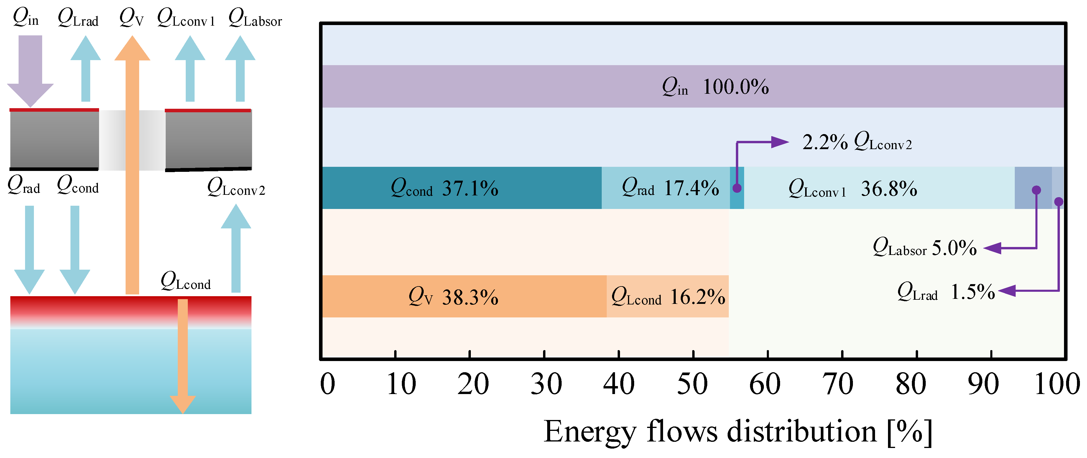
3.4.1. Energy Flow Analysis

To achieve the heat loss suppression of the scalable SCE process, the energy flows distribution of absorber–emitter and water surface was obtained. As solar absorber temperature increase, the heat transfer process is initiated. For the solar-absorber, the energy flows mainly include energy input Q_in, energy transferred to the water surface by heat conduction Q_cond and heat radiation Q_rad, the heat losses by convection Q_Lconv1 and thermal radiation Q_Lrad from the absorber surface transmit to the ambient and the convective heat losses Q_Lconv2 resulting in the heat transfer between the vapor and high-temperature absorber–emitter. For the water surface, the energy flows mainly include: Q_cond, Q_rad, latent heat of evaporation Q_v and the conduction heat loss Q_Lcond dissipated to the ambient through bulk water. For scalable SCE, the energy balance on solar absorber surface and water surface are shown in Equations (15) and (16).

$$Q_{\mathrm{in}}=Q_{\mathrm{cond}}+Q_{\mathrm{rad}}+Q_{\mathrm{Lconv}1}+Q_{\mathrm{Lconv}2}+Q_{\mathrm{Lrad}}$$

(15)

$$Q_{\mathrm{cond}}+Q_{\mathrm{rad}}=Q_{\mathrm{v}}+Q_{\mathrm{Lcond}}$$

(16)

Figure 11 shows the energy flows distribution of absorber–emitter and water surface during heat transfer in scalable SCE process. Two key conclusions could be derived from the results. The first one is that two major heat-loss contributors can be identified: heat dissipated to the ambient through the bulk water Q_lcond (16.2%) and heat losses by convection Q_Lconv1 from the absorber surface transmit to the ambient. The other is that the obtained heat of the water surface is mainly comes from the heat conduction (37.1%) rather than the radiation (17.4%) from the infrared emitter. The above analysis indicates that the evaporation rate of the scalable SCE could be effectively enhanced by proper ways to suppress the heat loss of Q_lcond and Q_Lconv1 or improve the efficiency of heat conduction in air layer.

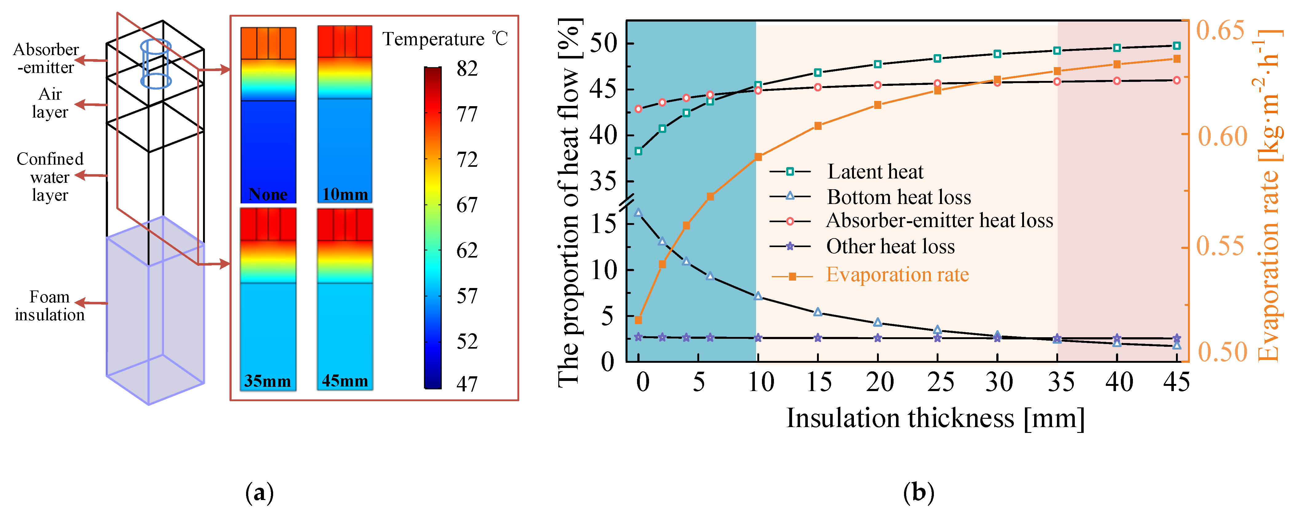
3.4.2. Heat Loss Suppression on the Water Side

In order to reduce heat loss on the water side, a layer of foam insulation was added starting from 5 mm below the water surface. The cross-sectional temperature distribution of the absorber–emitter, straight hole, air layer and 5 mm thick water layer under different foam insulation thicknesses of 0 mm, 10 mm, 35 mm and 45 mm is shown in Figure 12a. When the thickness increases from 0 mm to 10 mm, the overall temperature of the absorber–emitter, vapor diffusion hole and air layer rise significantly, indicating that the foam insulation layer plays an effective role in suppressing heat loss on the water side. However, when the thickness increases from 35 mm to 45 mm, the temperature rise of absorber emitter and air layer is slight. To further explore the relationship between evaporation rate and foam insulation layer thickness, the heat flow distribution under different foam insulation layer thickness was analyzed, as shown in Figure 12b. The results show that the convective heat loss on the absorber surface and other heat losses rise slightly as the foam insulation increases, mainly due to the temperature increase of the absorber–emitter. In addition, when the foam insulation layer thickness increases, the bottom heat loss can be divided into three stages: The first stage is the rapid decline stage, when the thickness of foam insulation layer increases from 0 mm to 10 mm, the bottom heat loss decreases from 16.1% to 7.1%. The second stage is the gentle decline stage, when the thickness of the foam insulation layer increases from 10 mm to 35 mm, the conduction heat loss decreases from 7.1% to 2.4%. The third stage is the slow decline stage, when the thickness of foam insulation layer increases from 35 mm to 45 mm, the bottom heat loss only decreases from 2.4% to 1.7%. The variations of the latent heat proportion and evaporation rate are opposite to that of bottom heat loss. The evaporation rates are 0.595 kg·m⁻²·h⁻¹, 0.645 kg·m⁻²·h⁻¹, and 0.652 kg·m⁻²·h⁻¹ at the thicknesses of the insulation layer are 10 mm, 35 mm and 45 mm, respectively. It can be deduced from the above analysis that the insulation layer thickness has an optimal value (35 mm) to take into account the economy and insulation performance.

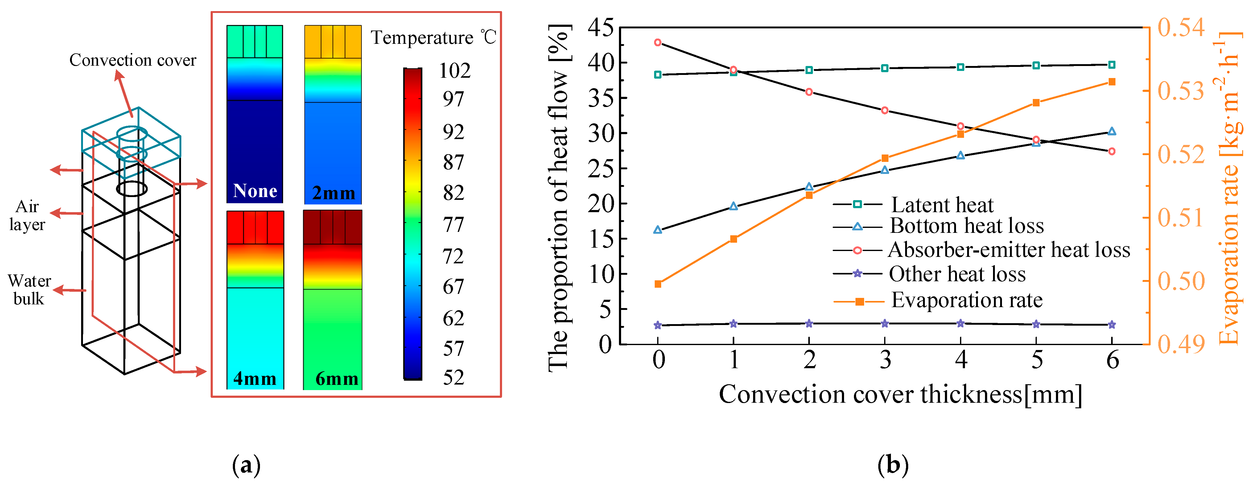
3.4.3. Heat Loss Suppression on the Air Side

An air-filled convection cover that matches the size of the absorber-emitter is used on the absorber surface to minimize heat loss through the air side. Straight holes are drilled on the convection cover to make sure the vapor escape from the absorber–emitter. The thermal conductivity of convection cover is set to be the same as that of air, and the radiative transmittivity is set to 100% in the simulation. Figure 13a shows the design of the scalable SCE, which includes a convection cover, as well as the cross-sectional temperature distribution of the absorber-emitter, vapor diffusion hole, and air layer. The thickness of the convection cover varies between 0 mm, 2 mm, 4 mm, and 6 mm, as shown in the figure. When the thickness of the convective cover increases, the overall temperature of the absorber–emitter, vapor diffusion hole, air layer and the 5 mm thick water layer rise significantly, indicating that the convection cover can effectively reduce the absorber–emitter heat loss. Given the fact that high convective cover thickness will improve vapor diffusion resistance and cause low transmittance, this study only explores the influence of convective cover plate thickness from 0 mm to 6 mm on the evaporation rate. The variation trends of the energy distribution ratio and evaporation rate with the increase in convection cover thickness are shown in Figure 13b. It can be seen that the evaporation rate increases from 0.499 kg·m⁻²·h⁻¹ to 0.531 kg·m⁻²·h⁻¹ with the increase in the convection cover thicknesses from 0 mm to 6 mm. Although the convective cover can effectively reduce the heat loss in air side, at the same time, the rise of water surface temperature will make the bulk water heat loss greatly increases, which leads to the proportion of latent heat used for evaporation increase slightly. Based on the above analysis, it can be concluded that, for the scalable SCE, adding only a convection cover will inevitably cause an increase in heat loss though the bulk water. Therefore, to achieve a significantly improved evaporation rate in the scalable SCE, it is necessary to use both a convection cover and a foam insulation layer simultaneously. The highest evaporation rate reaches 0.797 kg·m⁻²·h⁻¹ (η = 50.3%) when the thickness of insulation layer is 35 mm, and the thickness of the convection cover is 6 mm.

4. Conclusions

SCE promises to achieve ZLD without solar absorber contamination; however, this was only demonstrated with a small-scale laboratory device. This is partially limited by the illumination area of the solar simulator and cannot directly support its scalable adoption in a real-world application. To analyze the feasibility and potential of ZLD in a scalable application scenario, it is essential to understand the complicated transport mechanisms and analyze SCE with a precise modelling method. In this work, a comprehensive modelling framework of the SCE process was developed, considering the intertwined heat transfer, fluid flow and moisture transport. With the model validated by a laboratory evaporation test, parametric analysis of SCE was carried out. Energy and vapor transport behaviors, key heat-loss mechanisms, enhancing strategy and potential evaporation rate for scalable SCE were studied. Key conclusions drawn from the above studies are highlighted as follows:

(1)

Scalable SCE could obtain a higher evaporation rate (0.313 kg·m⁻²·h⁻¹) than the laboratory SCE (0.139 kg·m⁻²·h⁻¹), due to suppressed heat losses from the sidewalls;

(2)

Optimization of the hole parameter could increase the evaporation rate of scalable SCE up to 0.463 kg·m⁻²·h⁻¹, by tuning the competition between solar absorption and vapor diffusion;

(3)

The evaporation rate of scalable SCE could be further increased to 0.797 kg·m⁻²·h⁻¹, through the heat loss suppression both in water side and air side.

In summary, by proper design and additional thermal insulation for scalable SCE, the evaporation rate could be enhanced to 0.797 kg·m⁻²·h⁻¹, which is 473% higher than that of the laboratory SCE. This is also higher than the evaporation rate of a state-of-the-art design in SCE, indicating the promising potential of scalable SCE. The complex relationship between the vapor transport and heat transfer is formulated in the framework and critical trade-offs were investigated under various design scenarios. The experimentally validated modelling tool provides insights into the practical guidance on designing a scaled-up SCE device with heat transfer enhancements.

References

1. Mekonnen, M.M.; Hoekstra, A.Y. Four billion people facing severe water scarcity. Sci. Adv. 2016, 2, e1500323. [Google Scholar] [CrossRef] [PubMed] [Green Version]
2. Mclennan, M. INSIGHT REPORT in Partnership with the Global Risks Report 2021, 16th ed.; World Economic Forum: Cologny, Switzerland, 2021. [Google Scholar]
3. Vörösmarty, C.J.; McIntyre, P.B.; Gessner, M.O.; Dudgeon, D.; Prusevich, A.; Green, P.; Glidden, S.; Bunn, S.E.; Sullivan, C.A.; Liermann, C.R.; et al. Global threats to human water security and river biodiversity. Nature 2010, 467, 555–561, Erratum in Nature 2010, 468, 334–334. [Google Scholar] [CrossRef] [PubMed] [Green Version]
4. Demir, M.E.; Dincer, I. An integrated solar energy, wastewater treatment and desalination plant for hydrogen and freshwater production. Energy Convers. Manag. 2022, 267. [Google Scholar] [CrossRef]
5. Weifeng, H.; Yu, L.; Haohao, A.; Xuan, Z.; Pengfei, S.; Dong, H. Parametric analysis of humidification dehumidification desalination driven by photovoltaic/thermal (PV/T) system. Energy Convers. Manag. 2022, 259, 115520. [Google Scholar] [CrossRef]
6. Zhang, L.; Xu, Z.; Bhatia, B.; Li, B.; Zhao, L.; Wang, E.N. Modeling and performance analysis of high-efficiency thermally-localized multistage solar stills. Appl. Energy 2020, 266, 114864. [Google Scholar] [CrossRef]
7. Tong, T.; Elimelech, M. The Global Rise of Zero Liquid Discharge for Wastewater Management: Drivers, Technologies, and Future Directions. Environ. Sci. Technol. 2016, 50, 6846–6855. [Google Scholar] [CrossRef]
8. Lee, S.; Boo, C.; Elimelech, M.; Hong, S. Comparison of fouling behavior in forward osmosis (FO) and reverse osmosis (RO). J. Membr. Sci. 2010, 365, 34–39. [Google Scholar] [CrossRef]
9. Pinto, F.S.; Marques, R.C. Desalination projects economic feasibility: A standardization of cost determinants. Renew. Sustain. Energy Rev. 2017, 78, 904–915. [Google Scholar] [CrossRef]
10. Gude, V.G. Desalination and sustainability—An appraisal and current perspective. Water Res. 2016, 89, 87–106. [Google Scholar] [CrossRef]
11. Mohamed, A.; Maraqa, M.; Al Handhaly, J. Impact of land disposal of reject brine from desalination plants on soil and groundwater. Desalination 2005, 182, 411–433. [Google Scholar] [CrossRef]
12. Pramanik, B.K.; Shu, L.; Jegatheesan, V. A review of the management and treatment of brine solutions. Environ. Sci. Water Res. Technol. 2017, 3, 625–658. [Google Scholar] [CrossRef]
13. Shi, Y.; Zhang, C.; Li, R.; Zhuo, S.; Jin, Y.; Shi, L.; Hong, S.; Chang, J.; Ong, C.S.; Wang, P. Solar Evaporator with Controlled Salt Precipitation for Zero Liquid Discharge Desalination. Environ. Sci. Technol. 2018, 52, 11822–11830. [Google Scholar] [CrossRef] [PubMed]
14. Mickley, M. Survey of High-Recovery and Zero Liquid Discharge Technologies for Water Utilities; WaterReuse Found: Alexandria, VA, USA, 2008.
15. Bostjancic, J.; Ludlum, R. Getting to Zero Discharge: How to Recycle That Last Bit of Really Bad Wastewater A Brief History of Evaporation. Proc. Int. Water Conf. 1996, 57, 290–295. [Google Scholar]
16. Kashyap, V.; Al-Bayati, A.; Sajadi, S.M.; Irajizad, P.; Wang, S.H.; Ghasemi, H. A flexible anti-clogging graphite film for scalable solar desalination by heat localization. J. Mater. Chem. 2017, 5, 15227–15234. [Google Scholar] [CrossRef]
17. Xia, Y.; Li, Y.; Yuan, S.; Kang, Y.; Jian, M.; Hou, Q.; Gao, L.; Wang, H.; Zhang, X. A self-rotating solar evaporator for continuous and efficient desalination of hypersaline brine. J. Mater. Chem. 2020, 8, 16212–16217. [Google Scholar] [CrossRef]
18. Kuang, Y.; Chen, C.; He, S.; Hitz, E.M.; Wang, Y.; Gan, W.; Mi, R.; Hu, L. A High-Performance Self-Regenerating Solar Evaporator for Continuous Water Desalination. Adv. Mater. 2019, 31, e1900498. [Google Scholar] [CrossRef]
19. Zhang, C.; Shi, Y.; Shi, L.; Li, H.; Li, R.; Hong, S.; Zhuo, S.; Zhang, T.; Wang, P. Designing a next generation solar crystallizer for real seawater brine treatment with zero liquid discharge. Nat. Commun. 2021, 12, 998. [Google Scholar] [CrossRef]
20. Wang, W.; Aleid, S.; Shi, Y.; Zhang, C.; Li, R.; Wu, M.; Zhuo, S.; Wang, P. Integrated solar-driven PV cooling and seawater desalination with zero liquid discharge. Joule 2021, 5, 1873–1887. [Google Scholar] [CrossRef]
21. Ni, G.; Zandavi, S.H.; Javid, S.M.; Boriskina, S.V.; Cooper, T.A.; Chen, G. A salt-rejecting floating solar still for low-cost desalination. Energy Environ. Sci. 2018, 11, 1510–1519. [Google Scholar] [CrossRef]
22. Wang, W.; Shi, Y.; Zhang, C.; Hong, S.; Shi, L.; Chang, J.; Li, R.; Jin, Y.; Ong, C.; Zhuo, S.; et al. Simultaneous production of fresh water and electricity via multistage solar photovoltaic membrane distillation. Nat. Commun. 2019, 10, 3012. [Google Scholar] [CrossRef] [Green Version]
23. Xu, Z.; Zhang, L.; Zhao, L.; Li, B.; Bhatia, B.; Wang, C.; Wilke, K.L.; Song, Y.; Labban, O.; Lienhard, J.H.; et al. Ultrahigh-efficiency desalination via a thermally-localized multistage solar still. Energy Environ. Sci. 2020, 13, 830–839. [Google Scholar] [CrossRef] [Green Version]
24. Wang, Z.; Horseman, T.; Straub, A.P.; Yip, N.Y.; Li, D.; Elimelech, M.; Lin, S. Pathways and challenges for efficient solar-thermal desalination. Sci. Adv. 2019, 5, eaax0763. [Google Scholar] [CrossRef] [PubMed] [Green Version]
25. Chiavazzo, E.; Morciano, M.; Viglino, F.; Fasano, M.; Asinari, P. Passive solar high-yield seawater desalination by modular and low-cost distillation. Nat. Sustain. 2018, 1, 763–772. [Google Scholar] [CrossRef] [Green Version]
26. Gu, R.; Yu, Z.; Sun, Y.; Xie, P.; Li, Y.; Cheng, S. Enhancing stability of interfacial solar evaporator in high-salinity solutions by managing salt precipitation with Janus-based directional salt transfer structure. Desalination 2021, 524, 115470. [Google Scholar] [CrossRef]
27. Fan, Y.; Tian, Z.; Wang, F.; He, J.; Ye, X.; Zhu, Z.; Sun, H.; Liang, W.; Li, A. Enhanced Solar-to-Heat Efficiency of Photothermal Materials Containing an Additional Light-Reflection Layer for Solar-Driven Interfacial Water Evaporation. ACS Appl. Energy Mater. 2021, 4, 2932–2943. [Google Scholar] [CrossRef]
28. Yu, Z.; Gu, R.; Tian, Y.; Xie, P.; Jin, B.; Cheng, S. Enhanced Interfacial Solar Evaporation through Formation of Micro-Meniscuses and Microdroplets to Reduce Evaporation Enthalpy. Adv. Funct. Mater. 2022, 32. [Google Scholar] [CrossRef]
29. Thakur, A.K.; Sathyamurthy, R.; Velraj, R.; Lynch, I. Development of a novel cellulose foam augmented with candle-soot derived carbon nanoparticles for solar-powered desalination of brackish water. Environ. Sci. Nano 2022, 9, 1247–1270. [Google Scholar] [CrossRef]
30. Zhang, Q.; Yang, H.; Xiao, X.; Wang, H.; Yan, L.; Shi, Z.; Chen, Y.; Xu, W.; Wang, X. A new self-desalting solar evaporation system based on a vertically oriented porous polyacrylonitrile foam. J. Mater. Chem. 2019, 7, 14620–14628. [Google Scholar] [CrossRef]
31. Zhang, Q.; Hu, R.; Chen, Y.; Xiao, X.; Zhao, G.; Yang, H.; Li, J.; Xu, W.; Wang, X. Banyan-inspired hierarchical evaporators for efficient solar photothermal conversion. Appl. Energy 2020, 276, 115545. [Google Scholar] [CrossRef]
32. Xu, W.; Hu, X.; Zhuang, S.; Wang, Y.; Li, X.; Zhou, L.; Zhu, S.; Zhu, J. Flexible and Salt Resistant Janus Absorbers by Electrospinning for Stable and Efficient Solar Desalination. Adv. Energy Mater. 2018, 8. [Google Scholar] [CrossRef]
33. Liu, G.; Chen, T.; Xu, J.; Yao, G.; Xie, J.; Cheng, Y.; Miao, Z.; Wang, K. Salt-Rejecting Solar Interfacial Evaporation. Cell Rep. Phys. Sci. 2021, 2, 100310. [Google Scholar] [CrossRef]
34. Nawaz, F.; Yang, Y.; Zhao, S.; Sheng, M.; Pan, C.; Que, W. Innovative salt-blocking technologies of photothermal materials in solar-driven interfacial desalination. J. Mater. Chem. 2021, 9, 16233–16254. [Google Scholar] [CrossRef]
35. Cooper, T.A.; Zandavi, S.H.; Ni, G.W.; Tsurimaki, Y.; Huang, Y.; Boriskina, S.V.; Chen, G. Contactless steam generation and superheating under one sun illumination. Nat. Commun. 2018, 9, 1–10. [Google Scholar] [CrossRef] [PubMed] [Green Version]
36. Bertie, J.E.; Lan, Z. Infrared Intensities of Liquids XX: The Intensity of the OH Stretching Band of Liquid Water Revisited, and the Best Current Values of the Optical Constants of H2O(l) at 25°C between 15,000 and 1 cm−1. Appl. Spectrosc. 1996, 50, 1047–1057. [Google Scholar] [CrossRef]
37. Menon, A.K.; Haechler, I.; Kaur, S.; Lubner, S.; Prasher, R.S. Enhanced solar evaporation using a photo-thermal umbrella for wastewater management. Nat. Sustain. 2020, 3, 144–151. [Google Scholar] [CrossRef]
38. Zhang, L.; Xu, Z.; Zhao, L.; Bhatia, B.; Zhong, Y.; Gong, S.; Wang, E.N. Passive, high-efficiency thermally-localized solar desalination. Energy Environ. Sci. 2021, 14, 1771–1793. [Google Scholar] [CrossRef]
Figure 1. Schematic of the SCE. The red region in bulk water represents the penetration depth of infrared thermal radiation (~10 μm).
Applsci 13 04052 g001
Figure 2. Schematic diagrams of (a) the laboratory SCE device, (b) the scalable SCE device and (c) the detailed layout of absorber–emitter of both devices.
Applsci 13 04052 g002
Figure 3. Independence study of mesh for scalable SCE.
Applsci 13 04052 g003
Figure 4. Schematic diagram of the test rig for laboratory SCE.
Applsci 13 04052 g004
Figure 5. Temperatures from experiment and simulation results.
Applsci 13 04052 g005
Figure 6. Comparison between laboratory and scalable SCE. (a) Evaporation rates of SCE under different hole area ratios (0.7%, 14.4% and 36.9%). (b) Heat-balance analysis and key temperatures comparison of two SCE processes under a hole area ratio of 14.4%.
Applsci 13 04052 g006
Figure 7. Mechanism diagram of the downward heat transfer and the vapor diffusion for SCE.
Applsci 13 04052 g007
Figure 8. Tae, Twat-t and evaporation rate under different hole area ratios, with the same hole diameter (d = 1.1 mm) and air layer thickness (δ = 2.0 mm).
Applsci 13 04052 g008
Figure 9. Tae, Twat-t and evaporation rate under different hole diameters, with the same hole area ratio (φ = 20%) and air layer thickness (δ = 2.0 mm).
Applsci 13 04052 g009
Figure 10. (a) Tae, Twat-t and evaporation rate under different air layer thickness, with the same hole diameter (d = 1.1 mm) and hole area ratio (φ = 14%). (b) The temperature difference between the water surface and infrared emitter surface and the proportion of heat flow under different air layer thickness.
Applsci 13 04052 g010
Figure 11. Energy flows distribution of absorber–emitter and water surface during heat energy transfer from the top to bottom under the condition that the thickness of air layer is 2 mm, the hole diameter is 1.1 mm, and the hole area ratio is 14%.
Applsci 13 04052 g011
Figure 12. Potential of foam insulation to reduce conduction heat loss. (a) The structure of scalable SCE adding foam insulation and the cross-sectional temperature distribution of the absorber–emitter, vapor diffusion hole, air layer and 5 mm thick water layer under different insulation layer thicknesses of 0 mm, 10 mm, 35 mm and 45 mm. (b) The variation trends of energy distribution ratio and evaporation rate under different insulation layer thicknesses.
Applsci 13 04052 g012
Figure 13. Potential of a convection cover to reduce convection heat loss. (a) The structure of scalable SCE adding convection cover and the cross-sectional temperature distribution of the absorber–emitter, vapor diffusion hole and air layer under different convection cover thicknesses of 0 mm, 2 mm, 4 mm and 6 mm. (b) The energy flow distribution and evaporation rate under different convection cover thicknesses.
Applsci 13 04052 g013