Article

Estimation Strategy of RUL Calculation in the Case of Crack in the Magnets of PMM Used in HEV Application

1
College of Engineering and Technology, American University of the Middle East, Egaila 54200, Kuwait
2
Normandy University, UNIROUEN, ESIGELEC, IRSEEM, 76000 Rouen, France
3
LaRGES, Faculty of Engineering 1, Lebanese University, Tripoli 1300, Lebanon
*
Author to whom correspondence should be addressed.
Appl. Sci. 2023, 13(6), 3694; https://doi.org/10.3390/app13063694
Submission received: 30 January 2023 / Revised: 28 February 2023 / Accepted: 7 March 2023 / Published: 14 March 2023
(This article belongs to the Special Issue Focus on Fatigue and Fracture of Engineering Materials)

Abstract

:
Knowing the importance of assuring their reliability and availability, prognosis and remaining useful life calculation (RUL) concepts are highly suggested to be applied in critical applications such as hybrid electric vehicles (HEV). In the electrical propulsion system of HEVs, the electrical machine is one of the most critical elements considering its cost and function. Most electrical machines used in HEVs are permanent magnet machines (PMM). Most severe faults in PMM that affect its normal operation are the result of demagnetization. However, applying prognosis to a real prototype to detect the presence of mechanical defects such as cracks in the magnet of PMM and calculating the RUL of this defective element are challenging. In this paper, we are going to take advantage of a finite element model already built for the PMM in the healthy state and the state where cracks of different depths are integrated into the magnet. After that, relevant vital parameters that are affected when this type of fault persists in the machine are collected. Then, prognosis is applied to detect the presence of the crack in one piece of magnet in the electrical machine. Following this, the RUL calculation is performed to predict the remaining time before the crack propagates and a total fracture occurs in the magnet. The method used to execute the prognosis is the hidden Markov model (HMM). The RUL calculation will be performed using Paris equation, being the most important equation that models the growth and propagation of cracks

1. Introduction

Prognosis and RUL calculations are imperative perceptions to assure the healthy operation of systems and predict its total failure long before it occurs [1,2,3]. Hence, applying prognosis in critical applications such as HEV becomes mandatory [2]. There are three categories of prognostic methods: heuristic, model-based, and data-based methods [4,5,6,7,8,9].
HMM is a useful data-based prognostic method to predict the sequence of state changes in a system based on the sequence of observations. Hence, it is recommended for systems having a finite internal states that generate a set of external observations. The internal states of the system are invisible to an outward observer. The current state is directly dependent on the immediate previous state; this sequence is called the Markov process [10,11].
Many researchers started applying HMM for diagnosis and prognosis of electrical and mechanical faults in electrical machines [12]; the considered mechanical fault is mainly a crack in the bearing. However, none applied prognosis when faults such as demagnetization, being the most severe fault in machines such as permanent magnet machines [13], are integrated.
In paper [14], the author highlights the importance of detecting imminent faults in electric machines used in critical applications such as hybrid electric vehicles and avionics. It proves that hidden Markov model, used in diagnostics, is useful to be used as a prognostic technique. It presents two methods based on the hidden Markov models for the prediction of coming faults. They are based on pattern recognition, which is a data-driven approach commonly used in the field of faults recognition and diagnostic.
Paper [15] applies prognosis techniques to detect electrical faults using a hidden Markov model and estimates the remaining useful life of relevant equipment using an estimation approach based on the probability of state failure. The observables of the model are time and frequency features extracted from the machine’s torque measurement. To train the HMM, experimental observation probability densities are used due to limited available data. The investigated fault is a turn-to-turn short circuit; the research aims to detect the presence of turn-to-turn short circuits and estimate their severity from the extracted torque features.
The author in [11] declares that HMM is an advantageous method in diagnosis, prognosis, and condition monitoring fields. Currently, the wide availability of different types of sensors (vibration, temperature, torque) encourage researchers to apply HMM. It has been noted that HMMs can still be useful even if little training data and little prior knowledge about the system exists. In this paper, the observed data are the current of the electric motor. This measured parameter is used to detect the presence of faults, define the current state of the machine, and predict its future state.
The remaining useful life calculation is a new important concept that is beneficial to be applied in all electrical fields [16]. The RUL calculation and estimation for different elements constituting the electrical system of electric and hybrid electric vehicles is relatively new; however, it is becoming mandatory to assure health and proper operation [17,18,19,20]. In [21], the author highlights the importance of prognosis and RUL calculation specially for particular systems such as electrical machines in industrial applications. A data-driven prognostics method is used where a health index (HI) is proposed to predict the RUL of the selected electrical machine. Results show the advantage of this method over the traditional direct RUL prediction.
In hybrid electric vehicle applications, most researchers that discuss the RUL calculation apply it to the battery of the system. In [22], the RUL calculation is performed for a lithium battery used in a hybrid electric vehicle. The RUL estimation evaluate consecutive probability distributions of degrading battery states where a particle filter algorithm is built.
Knowing the importance of electrical machines in the functional operation of the electric propulsion system, prognosis and RUL calculations are crucial for hybrid electric vehicles in general and for used electric machines specifically [23,24,25].
Permanent magnet machines are widely used and advantageous in HEV applications [26] compared to other types of electrical machines due to their high efficiency, high power density, and simple construction [27,28,29,30].
It is hard to find a prototype for electrical machines where cracks are easily integrated for the aim of monitoring and collecting data for selected parameters that are affected by this type of fault, such as torque, current, temperature, and vibration [31,32,33] This is why in [34,35,36], a finite element model (FEM) of surface PMM is built; the electromagnetic, thermal, and vibration aspects of the machine are encountered. Additionally, in [37], a global HMM is built with the aim of detecting several types of faults in PMM: demagnetization represented by a crack in one piece of magnet in the machine, turn-to-turn short-circuit faults in one slot and eccentricity faults.
In this paper, two novel ideas will be discussed. Firstly, we present a strategy for computing the remaining useful life (RUL) related to a permanent magnet machine for the case where there is a crack in one of the magnets of the machine. Secondly, it is typically difficult to collect real-time data from a machine that gradually transitions from operating normally to becoming faulty over time due to a primitive fault. To this end, we utilize the finite element method for machines, as reported in [34,35,36]. The proposed FEM is validated via comparisons with the analytical model of machines in [34]. The FEM is an accurate way to model the electrical machine but in a specific state with no change in the physical aspect of the machine. To alleviate this problem, we combined this FEM with the Paris equation, which is a mature model for crack propagation.
In this study we will consider the demagnetization fault where a tiny crack of 1 mm will be integrated in one magnet of the PMM. Then, a remaining useful life calculation strategy will be presented. This strategy will permit the calculation of the RUL before total failure of the defective element occurs after detecting the presence of the elementary crack using the HMM previously described in [37].
In Section 2, we will present the physical characteristics of the machine used. The modeling of the crack growth will be shown in Section 3. In Section 4, estimation strategy of RUL calculation will be discussed using a database model. In Section 5, the generated model will be applied on the selected surface PMM where the results will be illustrated.

2. The Electrical Machine Used

The electrical machine used in this study is a 15 kW, 12-pole surface permanent magnet machine used in medium hybrid electric vehicles [38]. The magnets have 4.5 mm radial length and they are made of Neodymium iron boron.
The model of the machine is constructed using finite element analysis, which is a widely used numerical model, being simple and accurate [31,39]. The electromagnetic, thermal, and vibration models of the machine are built. The inputs of the prognostic model, where the RUL will be calculated at its end, are torque, temperature, and vibration.
The model will be built for undamaged machines and for machines with radial cracks of different depths in one of the 12 magnets.
A two-pole section of the healthy machine’s laminated sheet is shown in Figure 1; it is developed using ‘MATLAB’. In Figure 2a, a meshed view of the laminated sheet with a zoom on the cracked magnet is presented. The depth of the crack in Figure 2a is 1 mm. The considered first faulty state of the machine is the machine with a 1 mm radial crack in one magnet. A crack with depth less than 1 mm is not considered because it is at this depth where a change in the air gap flux density, torque, temperature, and vibration is detectable compared to the healthy state of the machine.
The radial length of the surface magnet is 4.5 mm; yet, we chose the final state of the fault to be a radial crack of 4 mm depth in the magnet instead of 4.5 mm. Although a 4.5 mm crack depth is a representation of a total fracture of the magnet, modeling it will cause a major change in the topology of the machine. In all cases, the end purpose of this study is ‘prognosis’. Hence, the suggested approach is supposed to detect the presence of this fault before a total failure occurs.
In Figure 2b, a meshed view of the laminated sheet where the crack deepens and becomes 4 mm is presented.
In Figure 3, Figure 4a,b, and Figure 5a,b we are illustrating the air gap flux density, in space, in the healthy case and in the case of 1 mm crack in the magnet as well as a 2 mm crack, 3 mm crack, and 4 mm crack.
In Figure 3, Figure 4a,b and Figure 5a,b, we can see the change in air gap flux density when the crack deepens to reach 4 mm depth. The torque of the machine is directly proportional to the air gap flux density. Hence, this proves that the torque is a good indicator for this type of fault.
In Figure 6, we are seeing the change in the vibration of the machine’s periphery, in the space domain, for the healthy case and for the case of cracks in the magnet. In Figure 7, the vibration in the case of 4 mm crack and the function of time are illustrated. Figure 6 and Figure 7 show that the vibration is a good indicator for the presence of this type of fault.
In Figure 8, the temperature on the machine’s periphery is illustrated in the healthy case and in the case of 1 mm crack in one magnet. A zoomed view of Figure 8 is shown in Figure 9. In Figure 10, the variation in the temperature function of time in the presence of one crack in one of the twelve magnets is shown. We mention that the data are collected from a virtual sensor located at the outer periphery of the machine in the finite element model.
Although the variation in the temperature is not highly detectable for demagnetization fault, temperature will be considered as an input for the model because prognosis is detecting the fault before it occurs or when it occurs at a very small scale. The incidence of false alarm is high; accordingly, taking more than one indicator to figure out the type of fault is mandatory. Although temperature is not a highly detectable indicator for demagnetization fault, it is a high indicator for other types of faults such as turn-to-turn short-circuits, as illustrated in [37]. This shows that not detecting changes in temperature eliminates the prospect of certain types of faults and reduces the possibilities of machine states to encounter demagnetization. With observing other types of parameters, such as torque and vibration, the vision will become clearer and the right machine state will be predicted. This is the function that performs the hidden Markov model.

3. Modeling of Crack Growth

The study of crack propagation is of big interest in many applications. One of the most important equations that models the growth and propagation of cracks is the Paris equation.
In fact, there are several models for the growth of cracks, such as the Paris, Duggan, Forman, and Tzamtzis models. Each one has its advantages and disadvantages. However, the Paris equation is the simplest, most famous, well-known, and mature model [40].
In [41], the Paris law equation is used in aircraft application. They are concerned with aging of critical material in aircraft function of time. Experimental testing of aircraft material is very important; however, constant material properties are not enough to evaluate materials in such critical applications. Hence, they evaluate materials according to their dynamic capability to develop and propagate cracks.
The author in [42] used the Paris equation to study crack growth and predict the remaining useful life of materials composing a magnet. In [43], the author use it for crack propagation in microelectronic device applications.
A crack growth rate is assessed for magnet systems in [44]. The paper was concerned with studying cracks with different orientations and different shapes. To realize this delicate modeling, the dual boundary element method and finite element method are coupled.
When applying the Paris equation for crack growth prediction, some assumptions need to be made:
  • The crack is not of constant amplitude; it is propagating a function of time;
  • The crack is one-dimensional;
  • The material where the crack exists has a certain elastic condition;
  • The load range is relatively constant;
  • Sensor data and offline signals have similar time stamps;
  • The offline data set contains enough data that represent different degradation behaviors.
According to the Paris law equation, the general fatigue crack growth model is:
d a d N c = C   Δ K n
Δ K = K m a x K o p
K o p = Q σ     π a 2
Q = cos π   a 2 W 1 2
d a d N c ’ is the crack growth rate.
‘a’ is the depth of the crack. ‘Nc’ is the number of cycles.
‘C’ and ‘n’ are calibration parameters dependent on the type of material where the crack is propagating. ‘C’ is called the Paris equation parameter or crack growth coefficient, its unit is [mm/(MN m−3/2)n] per cycle. ‘n’ is called the Paris equation exponent or crack growth exponent, and it is unitless.
‘∆K’ is the effective stress intensity factor. ‘Kmax’ is the stress intensity factor at the peak load; it is a critical or a threshold value before the occurrence of a fracture. ‘Kop’ is the operating stress intensity.
Maxwell stress tensor ‘σ’ will be calculated from the vibration FEM.
‘Q’ is a parameter dependent on the geometry of the system.
‘W’ is the radial length of the magnet.
A familiar relation between Nc and a is:
N c = 1 C   Δ σ   π   Q n 1 n 2 1 1 a 0 n 2 1 1 a f n 2 1
‘Nc’ is a cyclic loading, and it is a cycle representation of repetitive or inconsistent stress intensities on a certain location. ‘a0’ is the current depth of the crack. ‘af’ is the final depth that will reach the crack and at which the magnet is fractured.
Nc, calculated according to the above equation, is the RUL for the crack to move from a0 to af depth.
If we aim to calculate the time needed for the crack to propagate from 1 mm depth to a specific incremental depth, let us say 2 mm, the final state of the crack ‘f’ in this case is 2 mm.

4. Estimation Strategy of RUL Calculation Using Database Model

4.1. Description of the RUL Strategy

According to the literature, calculating RUL using database models consists of the following steps [45]:
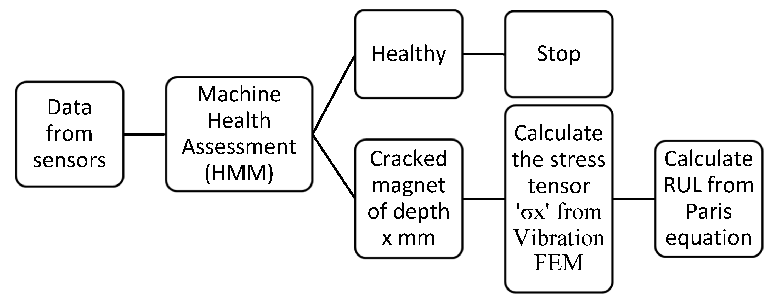
  • First, an offline database is prepared where data related to each phase of fault is encountered.
  • Second, a health assessment of the machine is conducted. In our case, the HMM model performed this assessment [37].
  • Third, the RUL calculation or prediction is executed.
At start, the offline database is elaborated from an executed simulation on real prototype or an equivalent model; in this research, we are going to use an already-built finite element machine model. Then, during the condition monitoring of the system’s operation, similarities between online and offline data sensors are tracked and detected. This can be performed by classification or regression [46].
Classification consists of matching data coming from sensors to one of the training data sets we already earned, where each set represents a specific state of the system [47].
Regression consists of predicting the real data from the sets of training data where a relation between these training data are created since the system phase of each set is known.
In our case, we will use ‘classification’ because online data coming from sensors can be generated from the previously developed dynamic FEM model of the machine [34,35].
Although dynamic FEM is the best real-time representation of the machine performance during healthy and faulty operation, alone it cannot generate online data useful for RUL calculation. Offline data samples can be generated for different machine states as much as needed. For example, the model can generate data representing vibrations detected by a vibration sensor when the machine is healthy, when the machine encounters a 1 mm crack in one magnet, and when the machine encounters a 2 mm crack in one magnet. However, when sampling data representing this vibration when the machine moves from the healthy state to the state of 1 mm crack in one magnet, the state where the crack worsens and becomes 2 mm is not possible. In other words, a model of the machine having any depth of the crack is possible using FEM; however, the time needed for the machine to shift from a faulty state with ‘x’ mm crack to a state with ‘y’ mm crack where y > x is not offered in FEM. In FEM, there is no representation of the fault propagation function of time.
Hence, many researchers combine the database approach and model based approach to build a rugged strategy for RUL calculation. Data sets for the database approach are generated from analytical analysis and numerical analysis such as FEM. The model-based method is formulated from the physical understanding of the system where a profound knowledge and an accurate representation of the fault propagation, the function of time, are presented.
If offline data correspond to the machine life cycle starting with its healthy state, then during the existence of tiny cracks in the magnet until the cracks worsen and become a fracture, the RUL calculation becomes easy. Such offline data could be represented in a data matrix ODM as follows:
O D M = D M 01 D M 02 D M 0 n D M 11 D M 12 D M 1 n D M 21 D M 22 D M 2 n D M m 1 D M m 2 D M m n  
In the above matrix, ‘n’ is the number of sampling points and ‘m’ is the number of times, during the life cycle of the machine, the data sets are recorded.
The first row of the matrix ODM is the data set observed at t = t0, when the machine is healthy. The second row is the data set observed at t = t1, when there is 1 mm crack in the magnet. The mth row is the data set observed at t = tm, when the magnet is completely fractured.
Different machine learning algorithm such as K-NN and Gaussian process regression can be used to execute a health assessment of the system and then calculate RUL as proved in paper [48].
A comparison between the current measured data set and the offline data set will be conducted. The most similar offline data set refers to the current machine state. We assume that the future behavior of the current monitored system is the same as that acquired in the offline system.
The RUL is calculated:
R U L = E O L s e l e c t e d t m
‘EOLselected’ is the end of life time of the system being in the current faulty phase identified by the health assessment already conducted.
Such offline data are not available since they need a real monitored system that contains this propagating fault we are interested in. Hence, a suggested strategy, inspired from the above presented method, will be presented in the following section to calculate the RUL.

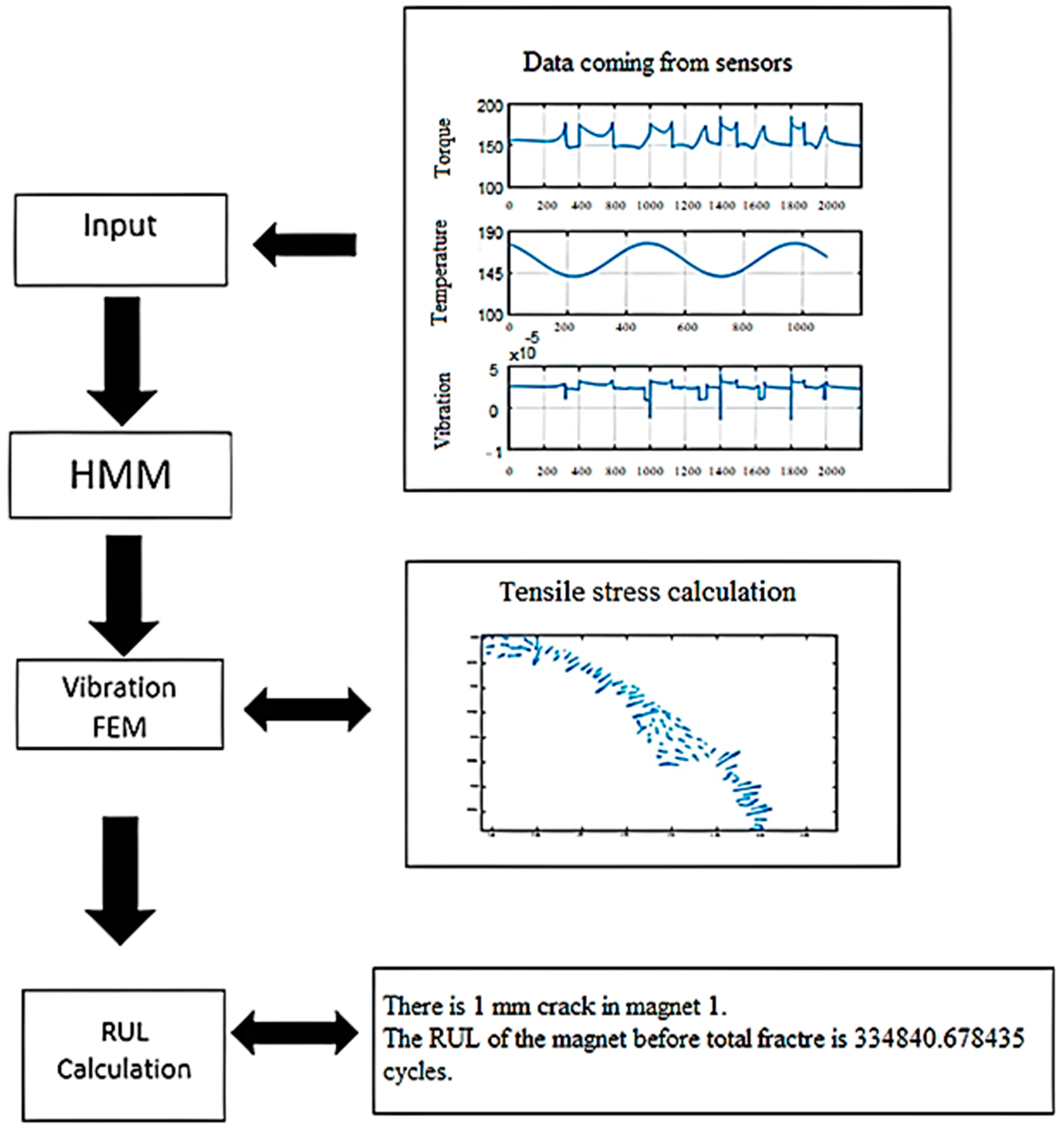
4.2. Adaptation and Application of the Described RUL above on Our System

In this research, we will use the above-described strategy to calculate the RUL in the case of cracks in one magnet; the system we are examining is a piece of a magnet in the PMM. The first detection of the fault will be when a crack of 1 mm depth is detected. RUL calculation is mainly the time needed for the faulty system to deteriorate. However, in our study, the final set of data will be collected in the case of 4 mm crack depth which is a near representation of the total fracture of the magnet.
First we will construct a synthetic offline database ‘SODM’. SODM will have the form of a matrix, as shown below:
S O D M = D S 01 D S 02 D S 0 t D S 11 D S 12 D S 1 t D S 21 D S 22 D S 2 t D S m 1 D S m 2 D S m t  
SODM represents sensor data in the healthy case and the case of cracks in a magnet inside the PMM. Its size is (m x t), where: ‘m’ is the number of states representing the systematic propagation of the studied fault, and ‘t’ is the number of sampling points.
The first row of matrix SODM is the data set for the case of 1 mm crack in the magnet along t sampling time. The second row is the data set for the case of 2 mm crack in the magnet along t sampling time. The mth row is the data set for the case of em mm crack in the magnet along t sampling time.
The difference between ODM and SODM is that the sets of data in ODM are extracted at a specific time during the life cycle of the machine; however, in SODM, the sets of data are extracted at an arbitrary time during a specific state of the machine.
Accordingly, each row of the SODM matrix is dedicated to sensor data at different depths of the magnet’s cracks. We started with a 1 mm crack depth and increase this depth, each time, by 1 mm until we reach em mm, which is the radial width of the magnet. At this depth the magnet is fractured.
We mention that the sampling times for all data sets are similar.
After constructing SODM, the first part of the suggested RUL calculation strategy is accomplished. The second part will be to find an appropriate equation that models the incremental growth of this fault, the cracks, and the function of time. This will be presented in the next section.
A block diagram illustrating the steps of the suggested strategy is illustrated in Figure 11.

5. The Application of the Strategy on the Selected System

In this research, we will consider a 4 mm depth as the final state of the magnet’s cracks before fracture, as we mentioned before.
At a time, data coming from torque, temperature, and vibration sensors are collected; their features will be inputs of the HMM model. These data are collected from dynamic FEM of the permanent magnet machine previously mentioned. The machine has a 235 mm outer diameter of stator, 145 mm outer diameter of rotor, and 195 mm axial length. The simulation is performed for five revolutions. The rotating step angle is 0.9 degrees, and the time step is 3.7425 × 10⁻⁵ s.
A decision will be generated from the HMM model; the state of the machine is either healthy or faulty. We mention that a percentage of reading error is examined for these selected sensors. The considered percentage error is ±0.5% for the torque sensor, ±0.55 ºC for the temperature sensor, and ±0.06% for the vibration sensor [49,50].
When the detected fault is a crack in one magnet, the model will identify the depth of the crack, and the RUL of the magnet needs to be calculated.
To perform this calculation, the vibration FEM is performed. Maxwell stress tensor ‘σ’ is computed from the vibration finite element model [35]. This calculated value is replaced in Equation (5) to calculate the RUL of the magnet.
An illustrative example of RUL calculation in the case of demagnetization due to 1 mm cracks in one magnet is presented in Figure 12.
In Table 1 and Figure 13, the RUL of the magnet, which is the remaining number of cycles ‘Nc’ before the magnet reaches its final state, is illustrated for different crack depths: 1 mm, 2 mm, and 3 mm. We notice that, as the cracks deepen, the number of cycles decreases because the RUL, before reaching the final state, decreases.

6. Conclusions

Many studies and statistics show that relying on hybrid electric vehicles will increase in the coming years due to many reasons such as the depletion of conventional sources of energy and environmental concerns. The causes of uneasiness regarding HEVs are their reliability and availability. To overcome this worry, several researchers stated the importance of detecting minor defects through prognosis and calculating the RUL of the system.
RUL is one of the most important parameters to be calculated in the case of defects in a system because it gives information on the time needed before this defect becomes a total failure and affects the operation of the studied system. Additionally, it helps in generating a decision on action needed after the occurrence of the defect. Answers to the following questions will be elaborated: Should we stop the system immediately? Is it cost effective to stop the system? How much time can this system still run before there is a total failure where corrective action needs to be taken?
In our studied case, the defect is a minor crack in one magnet in a surface permanent magnet machine used in hybrid electric vehicles. The health state of the magnet is very important in this application. The magnets are one of the essential elements in the permanent magnet machine that support the air gap magnetic field; subsequently, they support the generated torque and power.
The suggested RUL calculation study will calculate the time needed before the crack deepens and reach a graver state. This is performed after the detection of its presence using HMM model where torque, vibration, and temperature are used as model inputs.
The important factors for detecting the presence of preliminary cracks in the magnet and calculating their RUL before a total fracture occurs are: first, to know how long this machine can remain working, especially since a PMM with a crack in one magnet can still operate but with a lower efficiency; second, the possibility of taking a corrective action, which maybe repairing or replacing the cracked magnet.
The proposed strategy was able, after detecting the presence of preliminary cracks in one magnet by HMM, to calculate the remaining useful life of the defective piece of magnet.
In article [37], an RUL calculation for the same type of machine for the case of turn-to-turn short-circuit faults is presented. In this article, an RUL calculation strategy is suggested for the case of demagnetization faults. For the future, the work in this field to elaborate a global RUL calculation model encountering different types of faults that may occur in the electrical machine and in the whole electrical propulsion system of the vehicle is continuous.

Author Contributions

Writing—review & editing, R.G., G.H. and N.M. All authors have read and agreed to the published version of the manuscript.

Funding

This research received no external funding.

Data Availability Statement

Data available on request, from the corresponding author, due to privacy restrictions.

Conflicts of Interest

The authors declare no conflict of interest.

References

  1. Sankavaram, C.; Kodali, A.; Pattipati, K. An Integrated Health Management Process for Automotive Cyber-Physical Systems. In Proceedings of the IEEE International Conference on Computing, Networking and Communications, Workshops Cyber Physical System, San Diego, CA, USA, 28–31 January 2013. [Google Scholar]
  2. Yang, A.; Widodo, S. Introduction of Intelligent Machine Fault Diagnosis and Prognosis; Nova Science Publishers: Hauppauge, NY, USA, 2010. [Google Scholar]
  3. Djeziri, M.A.; Benmoussa, S.; Sanshez, R. Hybrid method for remaining useful life prediction in wind turbine systems. Renew. Energy 2018, 116, 173–187. [Google Scholar] [CrossRef]
  4. Ginzarly, R.; Hoblos, G.; Moubayed, N. Decision on Prognosis approaches of Hybrid Electric Vehicles’ electrical machines. In Proceedings of the 2015 Third International Conference on Technological Advances in Electrical, Electronics and Computer Engineering (TAEECE), Beirut, Lebanon, 29 April–1 May 2015. [Google Scholar]
  5. Ginzarly, R.; Hoblos, G.; Moubayed, N. Hidden Markov Model Based Failure Prognosis for Permanent Magnet Synchronous Machine. In ACD European Workshop on Advanced Control and Diagnosis; Springer: Florence, Italy, 2019. [Google Scholar]
  6. Eker, O.F.; Camci, F.; Jennions, I.K. Major Challenges in Prognostics: Study on Benchmarking Prognostics Datasets. In Proceedings of the 1st European Conference of the Prognostics and Health Management Society, Dresden, Germany, 3–5 July 2012; PHM Society. pp. 148–155. [Google Scholar]
  7. Guo, J.; Li, Z.; Li, M. A Review on Prognostics Methods for Engineering Systems. IEEE Trans. Reliab. 2019, 69, 1110–1129. [Google Scholar] [CrossRef]
  8. Djeziri, M.A.; Benmoussa, S.; Benbouzid, M. Data-driven approach augmented in simulation for robust fault prognosis. Eng. Appl. Artif. Intell. 2019, 86, 154–164. [Google Scholar] [CrossRef]
  9. Enrique, L.; Arroyo, C. Modeling and Simulation of Permanent Magnet Synchronous Motor Drive System. Master’s Thesis, University of Puerto Rico, Mayagüez Campus, Mayagüez, Puerto Rico, 2006. [Google Scholar]
  10. Rabiner, L. A tutorial on hidden markov model and selected applications in speech recognition. Proc. IEEE 1989, 77, 257–286. [Google Scholar] [CrossRef] [Green Version]
  11. Haider, S.; Zanardelli, W.; Aviyente, S. Prognosis of Electrical Faults in Permanent Magnet AC Machines using the Hidden Markov Model. In Proceedings of the IECON 2010-36th Annual Conference on IEEE Industrial Electronics Society, Glendale, AZ, USA, 7–10 November 2010. [Google Scholar]
  12. Mecrow, B.C.; Jack, A.; Haylock, J.; Coles, J. Fault-tolerant permanent magnet machine drives. IEE Proc.-Electr. Power Appl. 1996, 143, 437–442. [Google Scholar] [CrossRef]
  13. Winkler, D.; Gühmann, C. Modelling of Electrical Faults in Induction Machines Using Modelica. In Proceedings of the 48th Scandinavian Conference on Simulation and Modeling, Särö, Dennemark, 30–31 October 2007; pp. 82–87. [Google Scholar]
  14. Fettweis, G.; Meyr, H. Feedforward Architectures for Parallel Viterbi Decoding. J. VLSI Signal Process. 1991, 3, 105–119. [Google Scholar] [CrossRef] [Green Version]
  15. Heng, A.; Zhang, S.; Tan, A. Rotating machinery prognostics: State of the art, challenges and opportunities. Mech. Syst. Signal Process. 2009, 23, 724–739. [Google Scholar] [CrossRef]
  16. ShengSi, X.; Hu, W.W.C.; Zhouc, D. Remaining useful life estimation–A review on the statistical data driven approaches. Eur. J. Oper. Res. 2011, 213, 1–14. [Google Scholar]
  17. Wang, X.; Li, J.; Kao, B.-C.; Ho, Y.-W. A Novel Prediction Process of the Remaining Useful Life of Electric Vehicle Battery Using Real-World Data. Processes 2021, 9, 2174. [Google Scholar] [CrossRef]
  18. Wu, L.; Fu, X.; Guan, Y. Review of the Remaining Useful Life Prognostics of Vehicle Lithium-Ion Batteries Using Data-Driven Methodologies. Appl. Sci. 2016, 6, 166. [Google Scholar] [CrossRef] [Green Version]
  19. Pan, C.; Huang, A.; He, Z.; Lin, C.; Sun, Y.; Zhao, S.; Wang, L. Prediction of remaining useful life for lithium-ion battery based on particle filter with residual resampling. Energy Sci. Eng. 2021, 9, 1115–1133. [Google Scholar] [CrossRef]
  20. Li, X.; Shu, X.; Shen, J.; Xiao, R.; Yan, W.; Chen, Z. An O-Board remaining useful life estimation algorithm for Lithium Ion batteries of electric vehicles. Energies 2017, 10, 691. [Google Scholar] [CrossRef] [Green Version]
  21. Yang, F.; Habibullah, M.S.; Zhang, T.; Xu, Z.; Lim, P.; Nadarajan, S. Health Index-Based Prognostics for Remaining Useful Life Predictions in Electrical Machines. IEEE Trans. Ind. Electron. 2016, 63, 2633–2644. [Google Scholar] [CrossRef]
  22. Omariba, Z.; Zhang, L.; Sun, D. Remaining Useful Life Prediction of Electric Vehicle Lithium-Ion Battery Based on Particle Filter Method. In Proceedings of the IEEE 3rd International conference on Big Data Analysis, Shanghai, China, 9–12 March 2018. [Google Scholar]
  23. Chau, K.; Li, W. Overview of electric machines for electric and hybrid vehicles. Int. J. Veh. Des. 2014, 64, 46. [Google Scholar] [CrossRef] [Green Version]
  24. Finken, T.; Felden, M.; Hameyer, K. Comparison and design of different electrical machine types regarding their applicability in hybrid electrical vehicles. In Proceedings of the 2008 18th International Conference on Electrical Machines, Vilamoura, Portugal, 6–9 September 2008. [Google Scholar]
  25. Simpson, A. Cost-Benefit Analysis of Plug-In Hybrid Electric Vehicle Technology. In Proceedings of the 22nd International Battery, Hybrid and Fuel Cell Electric Vehicle Symposium and Exhibition (EVS-22), Yokohama, Japan, 23–28 October 2006. [Google Scholar]
  26. Zheng, J.; Zhao, W.; Ji, J.H.; Liu, G. Design and comparison of interior permanent-magnet machines for hybrid electric vehicles. In Proceedings of the IEEE International Conference on Applied Superconductivity and Electromagnetic Devices (ASEMD), Shanghai, China, 20–23 November 2015. [Google Scholar]
  27. Chan, C.C.; Chau, K.T.; Jiang, J.Z. Novel Permanent Magnet Motor Drives for Electric Vehicles. IEEE Trans. Ind. Electron. 1996, 43, 331–339. [Google Scholar] [CrossRef] [Green Version]
  28. Schneider, T.; Binder, A. Evaluation of new Surface Mounted Permanent Magnet Synchronous Machine with Finite Element Calculations. In Computer Engineering in Applied Electromagnetism; Springer: Dordrecht, The Netherlands, 2005. [Google Scholar]
  29. Hu, T.; Lin, F.; Cui, L. The Flux-Weakening Control of Interior Permanent Magnet Synchronous Traction Motors for High-Speed Train. In Proceedings of the 1st International Workshop on High-Speed and Intercity Railways; Lecture Notes in Electrical Engineering; Springer: Berlin/Heidelberg, Germany, 2012; volume 147. [Google Scholar]
  30. Wang, A.; Ma, D.; Wang, H. FEA-Based Calculation of Performances of IPM Machines with Five Topologies for Hybrid-Electric Vehicle Traction. Int. J. Electr. Comput. Electron. Commun. Eng. 2013, 7, 929–977. [Google Scholar]
  31. Lee, S.; Habetler, T.G. An online stator winding resistance estimation techniquefor temperature monitoring of line-connected inductionmachines. IEEE Ind. Appl. Conf. 2001, 39, 685–994. [Google Scholar]
  32. Hsu, J.S. Possible errors in measurement of air-gap torque pulsations of induction motors. IEEE Trans. Energy Convers. 1992, 7, 202–208. [Google Scholar] [CrossRef] [Green Version]
  33. Hsu, J.S. Monitoring of Defects in Induction Motors Through Air-Gap Torque Observation. IEEE Trans. Ind. Appl. 1995, 31, 1016–1021. [Google Scholar] [CrossRef] [Green Version]
  34. Ginzarly, R.; Alameh, K.; Hoblos, G.; Moubayed, N. Moubayed, Numerical versus analytical techniques for healthy and faulty surface permanent magnet machine. In Proceedings of the 2016 Third International Conference on Electrical, Electronics, Computer Engineering and their Applications (EECEA), Beirut, Lebanon, 21–23 April 2016. [Google Scholar]
  35. Ginzarly, R.; Hoblos, G.; Moubayed, N. Electromagnetic and vibration finite element model for early fault detection in permanent magnet machine. In Proceedings of the 10th IFAC Symposium on Fault Detection, Supervision and Safety of Technical Processes, Warsaw, Poland, 29–31 August 2018. [Google Scholar]
  36. Ginzarly, R.; Hoblos, G.; Moubayed, N. Localizing Turn to Turn Short Circuit in HEV’s Machine Using Thermal Finite Element Model. In Proceedings of the IEEE International Multidisciplinary Conference on Engineering Technology (IMCET), Beirut, Lebanon, 4–16 November 2018. [Google Scholar]
  37. Ginzarly, R.; Hoblos, G.; Moubayed, N. From Modeling to Failure Prognosis of Permanent Magnet Synchronous Machine. Appl. Sci. 2020, 10, 691. [Google Scholar] [CrossRef] [Green Version]
  38. Wu, Z. Conception Optimale d’un Entrainement Electrique Pour la Chaine de Traction d’un Vehicule Hybride Electrique. 21 Mars 2012. Available online: https://tel.archives-ouvertes.fr/tel-00838732 (accessed on 29 January 2023).
  39. Donea, J.; Huerta, A. Finite Element Methods for Flow Problems; Wiley: Hoboken, NJ, USA, 2004. [Google Scholar]
  40. Azaïs, R.; Gégout-Petit, A.; Greciet, F. Rupture detection in fatigue crack propagation. In Statistical Inference for Piecewise-deterministic Markov Processes; Wiley: Hoboken, NJ, USA, 2018; pp. 173–207. [Google Scholar]
  41. Klysz, S.; Gmurkzyk, G.; Lisiecki, J. Fatigue of Aircraft Structures; Institute of Aviation Scientific Publications: Warsaw, Poland, 2010; pp. 52–58. [Google Scholar]
  42. Wong, F. Fatigue, Fracture, and Life Prediction Criteria for Composite Materials in Magnets; Plasma Fusion Center Massachusetts Institute of Technology: Cambridge, MA, USA, 1990. [Google Scholar]
  43. Citarella, R.; Frattura, A.; Strutturale, F. Coupled FEM-DBEM method to assess crack growth in magnet system of Wendelstein. Frattura ed Integrità Strutturale 2013, 26, 92–103. [Google Scholar] [CrossRef] [Green Version]
  44. Jiang, S.; Zhang, W.; Li, X. An Analytical Model for Fatigue Crack Propagation Prediction with Overload Effect. Math. Probl. Eng. 2014, 2014, 713678. [Google Scholar] [CrossRef] [Green Version]
  45. Yu, Y.; Hu, C.; Si, X. Degradation Data-Driven Remaining Useful Life Estimation in the Absence of Prior Degradation Knowledge. J. Control. Sci. Eng. 2017, 2017, 4375690. [Google Scholar] [CrossRef] [Green Version]
  46. Mosallam, A.; Medjaher, K.; Zerhouni, N. Data-driven prognostic method based on Bayesian approaches for direct remaining useful life prediction. J. Intell. Manuf. 2014, 27, 1037–1048. [Google Scholar] [CrossRef] [Green Version]
  47. Torgo, L.; Zizka, J.; Brazdil, P. Data Fitting with Rule-based Regression. In Proceedings of the 2nd international workshop on Artificial Intelligence Techniques (AIT’95), Brno, Czech Republic, 18–20 September 1995. [Google Scholar]
  48. Rymarczyk, T.; Kłosowski, G.; Kozłowski, E. Comparison of Selected Machine Learning Algorithms for Industrial Electrical Tomography. Sensors 2019, 19, 1521. [Google Scholar] [CrossRef] [PubMed] [Green Version]
  49. Mohammed, A.; Djurovic, S. Stator Winding Internal Thermal Stress Monitoring and Analysis Using in-situ FBG Sensing Technology. IEEE Trans. Energy Convers. 2018, 33, 1508–1518. [Google Scholar] [CrossRef]
  50. Saha, A. FPGA based self-vibration compensated two-dimensional non-contact vibration measurement using 2D position sensitive detector with remote monitoring. In International Measurement Confederation; Institute of Measurement and Control; Elsevier: Amsterdam, The Netherlands, 2017. [Google Scholar]
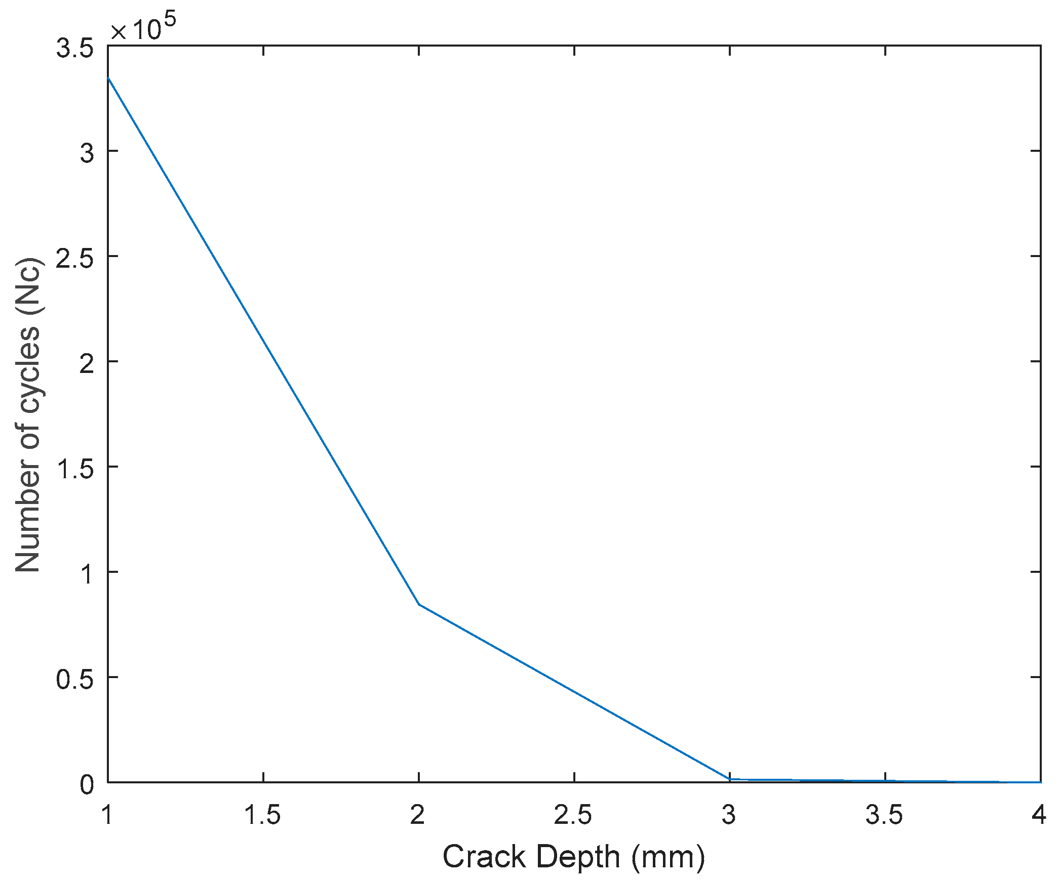
Figure 1. Two-pole section of the SPMM’s laminated sheet in healthy state.
Applsci 13 03694 g001
Figure 2. (a) Crack of 1 mm depth in the first magnet of pole 1 (meshed view). (b) Meshed laminated sheet with 4 mm crack in the magnet.
Applsci 13 03694 g002
Figure 3. Air gap flux density in the healthy case.
Applsci 13 03694 g003
Figure 4. (a) Air gap flux density with a 1 mm crack. (b) Air gap flux density with a 2 mm crack.
Applsci 13 03694 g004
Figure 5. (a) Air gap flux density with a 3 mm crack. (b) Air gap flux density with a 4 mm crack.
Applsci 13 03694 g005
Figure 6. Vibration on the machine’s periphery in the case of crack in the magnet.
Applsci 13 03694 g006
Figure 7. Vibration detected by the sensor in the case of 4 mm crack in the magnet.
Applsci 13 03694 g007
Figure 8. Temperature in the healthy case and in the case of 1 mm crack in the magnet.
Applsci 13 03694 g008
Figure 9. Zoomed view of Figure 8.
Applsci 13 03694 g009
Figure 10. Temperature at the machine’s periphery in the case of crack in one of the 12 magnets.
Applsci 13 03694 g010
Figure 11. RUL calculation in the case of demagnetization fault.
Applsci 13 03694 g011
Figure 12. Illustrative example of RUL calculation in the case of demagnetization due to 1 mm cracks in one magnet.
Applsci 13 03694 g012
Figure 13. Magnet number of cycles versus crack depth.
Applsci 13 03694 g013
Table 1. Magnet number of cycles versus crack depth.
Crack DepthRUL (Nc)
1 mm334,840.68
2 mm84,555.73
3 mm1423.5
4 mm0
Disclaimer/Publisher’s Note: The statements, opinions and data contained in all publications are solely those of the individual author(s) and contributor(s) and not of MDPI and/or the editor(s). MDPI and/or the editor(s) disclaim responsibility for any injury to people or property resulting from any ideas, methods, instructions or products referred to in the content.

