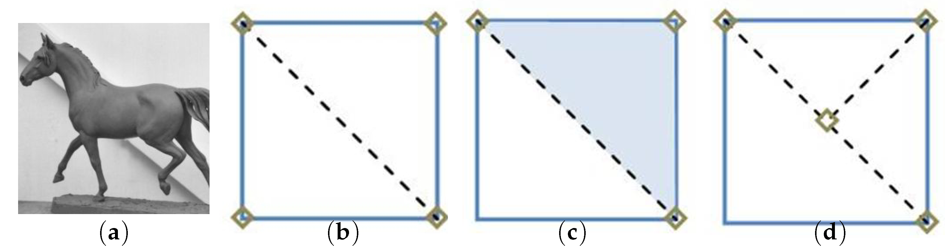
Figure 1.
BTTC process. (a) Original image. (b) Triangle division process. (c) Reconstruction of inner values by interpolation. (d) Repeated triangle division process.
Figure 1.
BTTC process. (a) Original image. (b) Triangle division process. (c) Reconstruction of inner values by interpolation. (d) Repeated triangle division process.
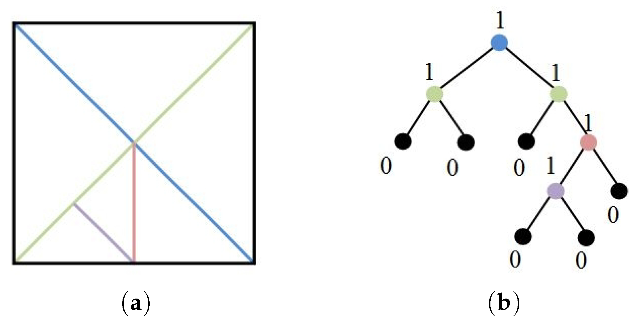
Figure 2.
Process of creating the B-tree structure. (a) Process of dividing the triangles. (b) Corresponding binary tree structure.
Figure 2.
Process of creating the B-tree structure. (a) Process of dividing the triangles. (b) Corresponding binary tree structure.
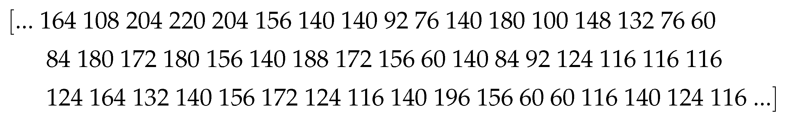
Figure 3.
Random part of the gray value stream acquired using the EEDC.
Figure 3.
Random part of the gray value stream acquired using the EEDC.
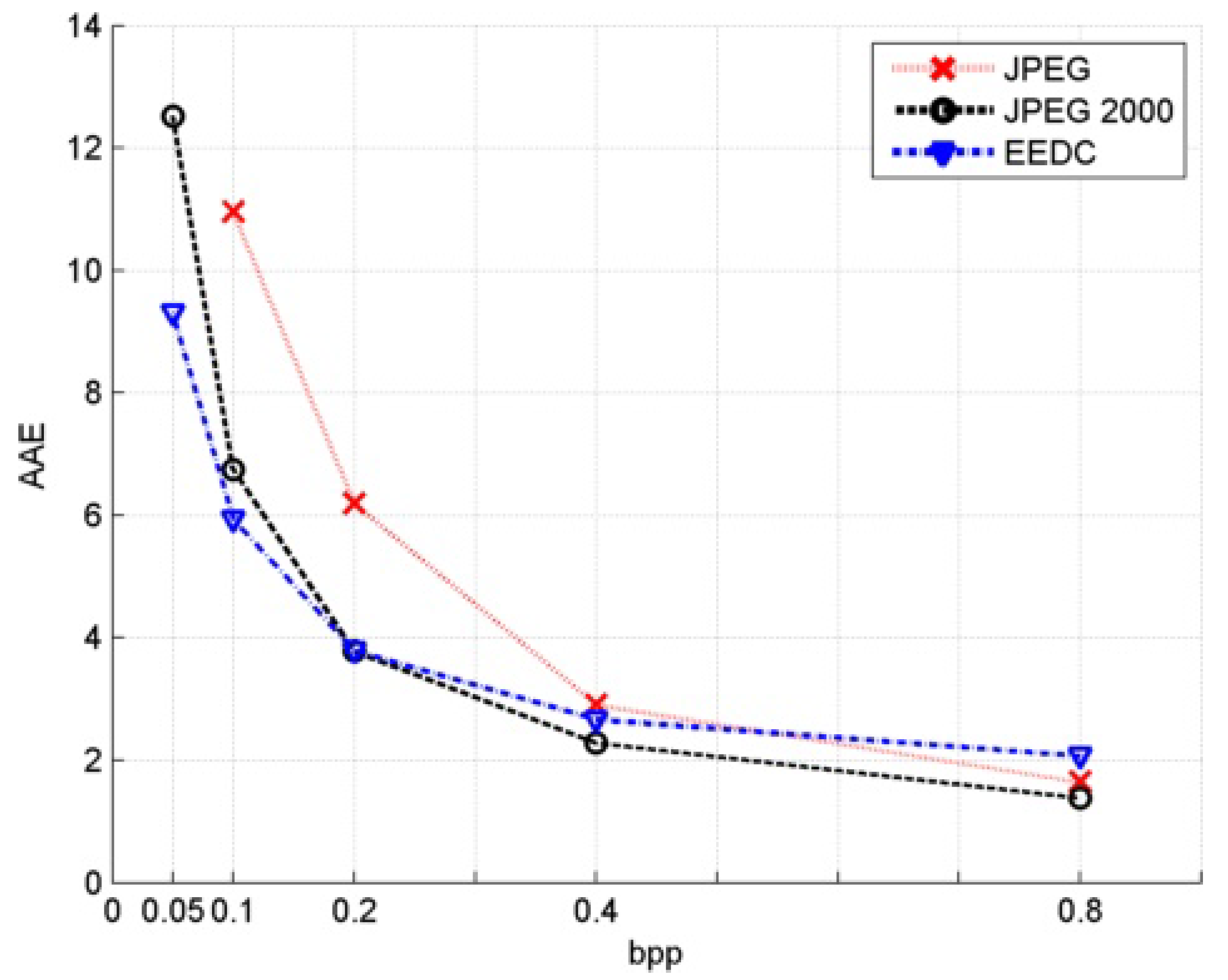
Figure 4.
AAE for image horse and unmodified gray value compression algorithm.
Figure 4.
AAE for image horse and unmodified gray value compression algorithm.
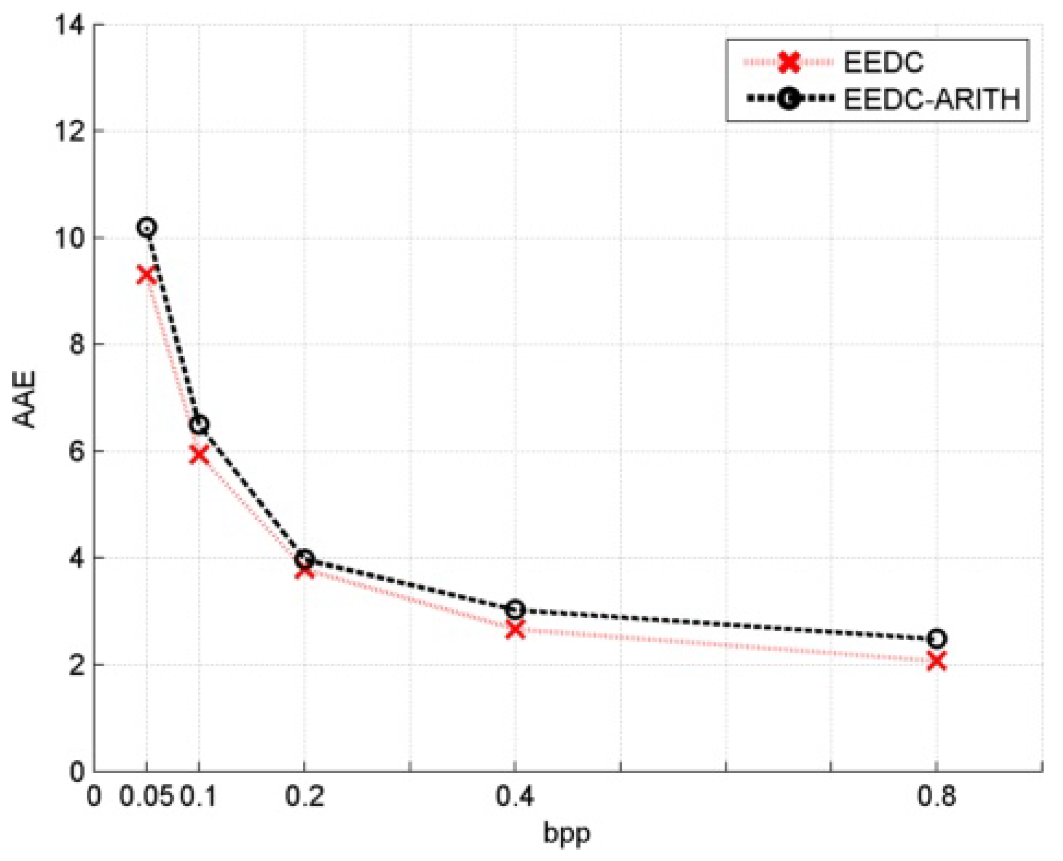
Figure 5.
AAE for image horse and modified gray values compression using arithmetic coding.
Figure 5.
AAE for image horse and modified gray values compression using arithmetic coding.
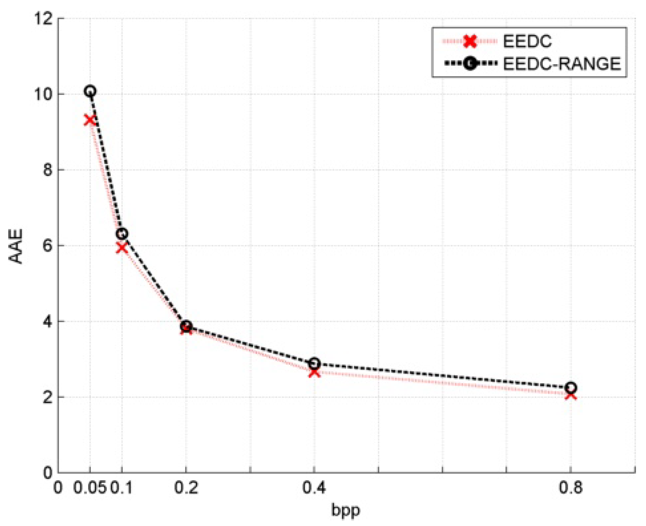
Figure 6.
AAE for image horse and modified gray values compression with range coding.
Figure 6.
AAE for image horse and modified gray values compression with range coding.
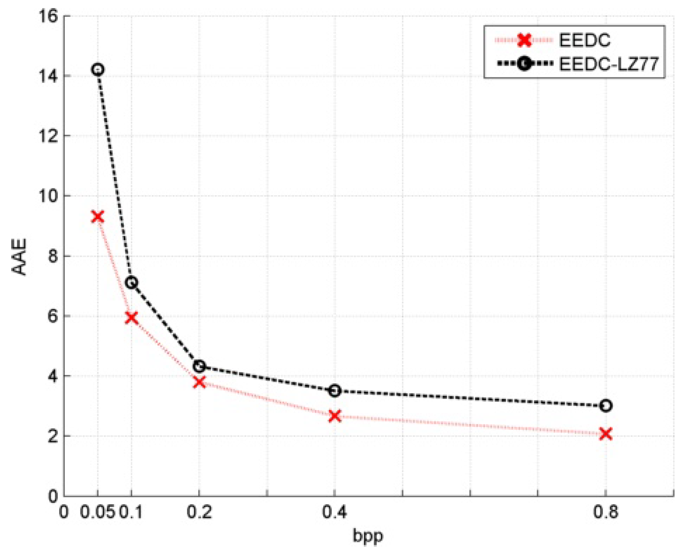
Figure 7.
AAE for image horse and modified gray values compression with LZ77 coding.
Figure 7.
AAE for image horse and modified gray values compression with LZ77 coding.
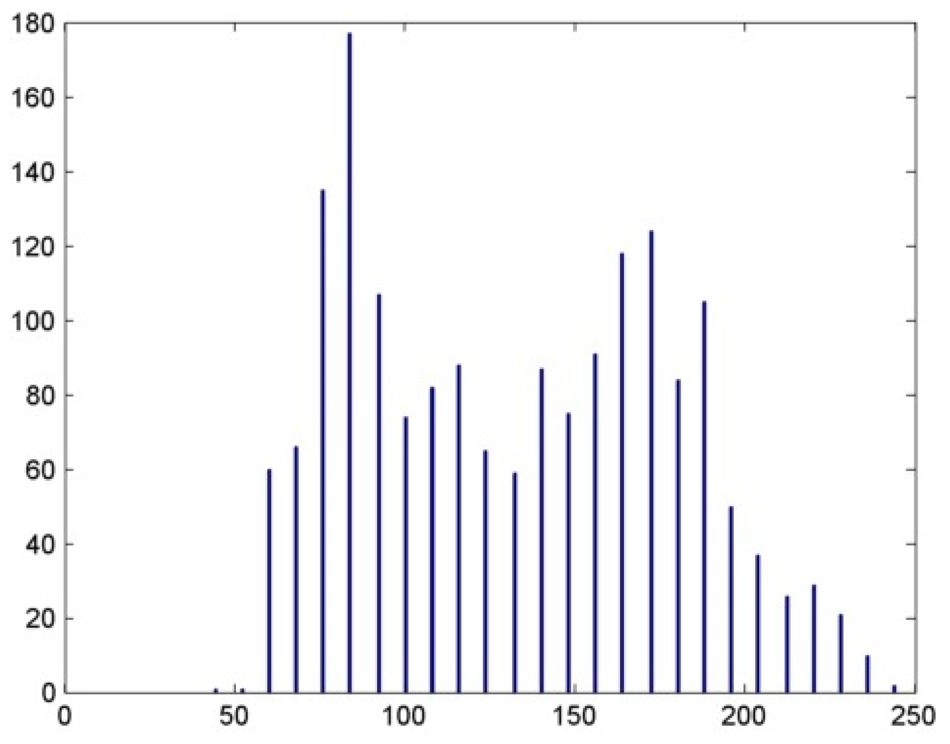
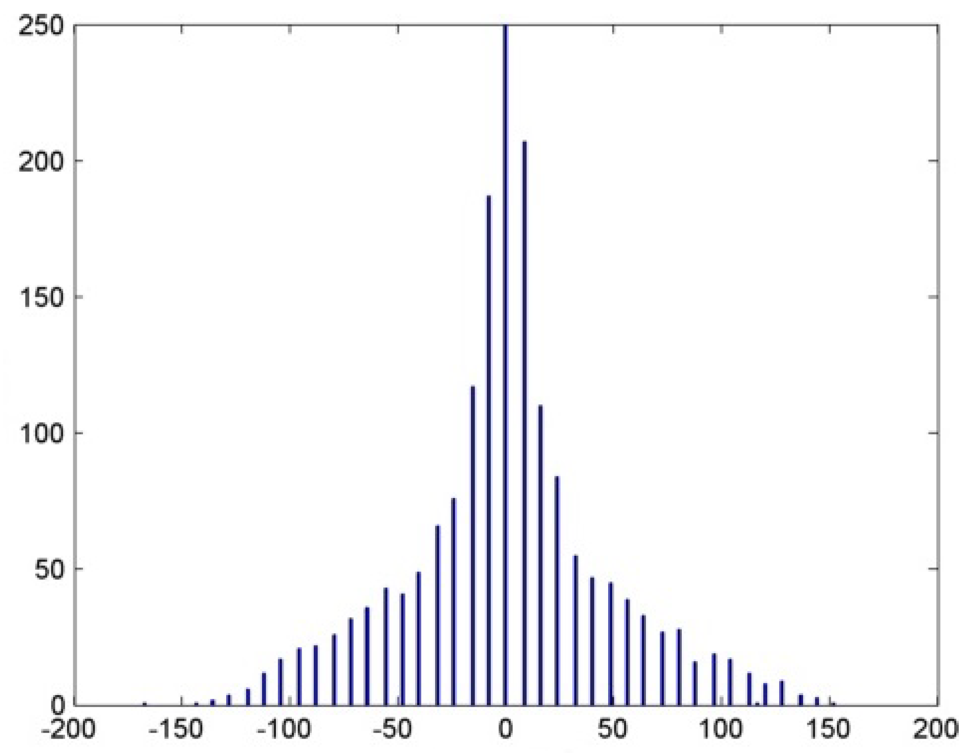
Figure 8.
Histogram of the image horse.
Figure 8.
Histogram of the image horse.
Figure 9.
Histogram of the image horse after applying delta coding.
Figure 9.
Histogram of the image horse after applying delta coding.
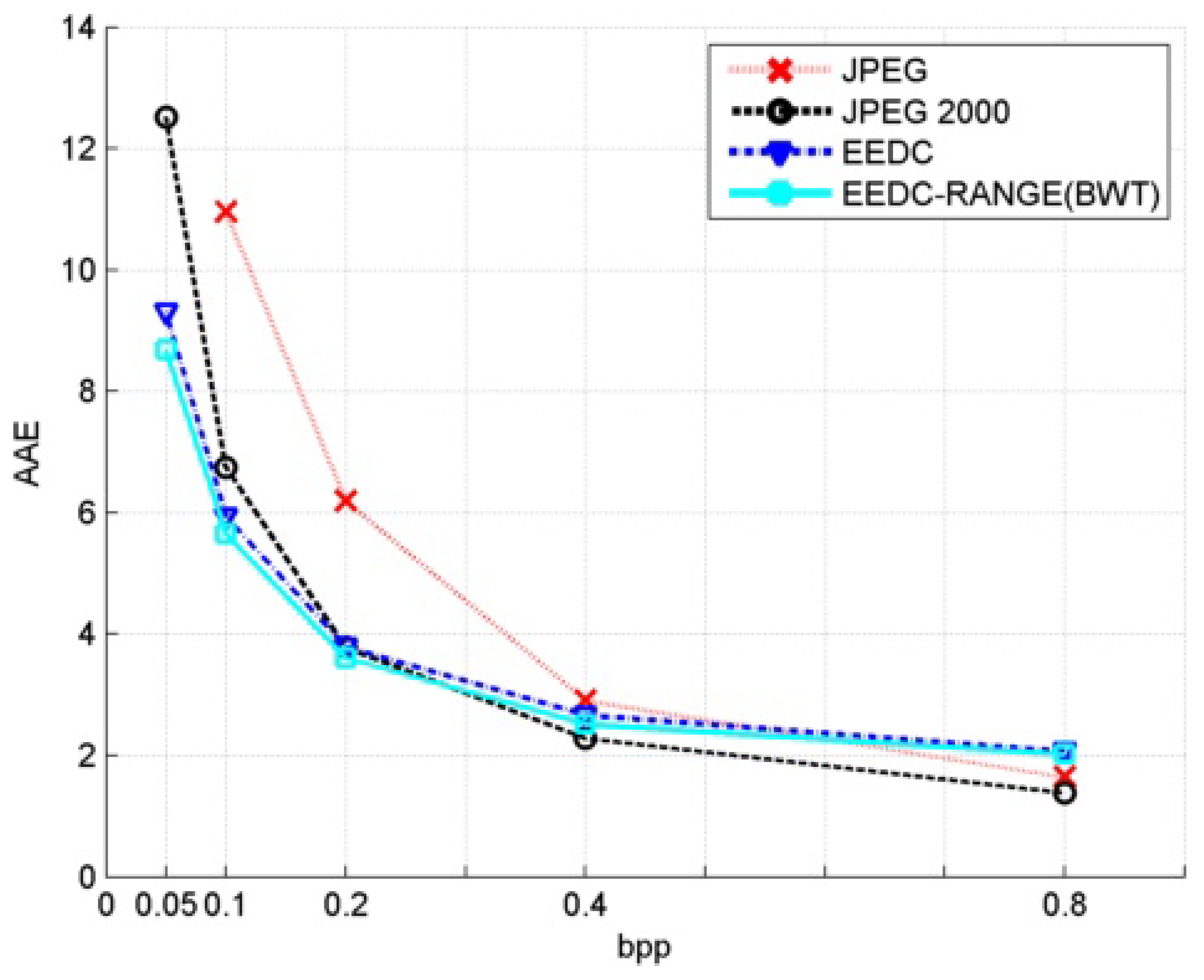
Figure 10.
AAE comparison for image horse.
Figure 10.
AAE comparison for image horse.
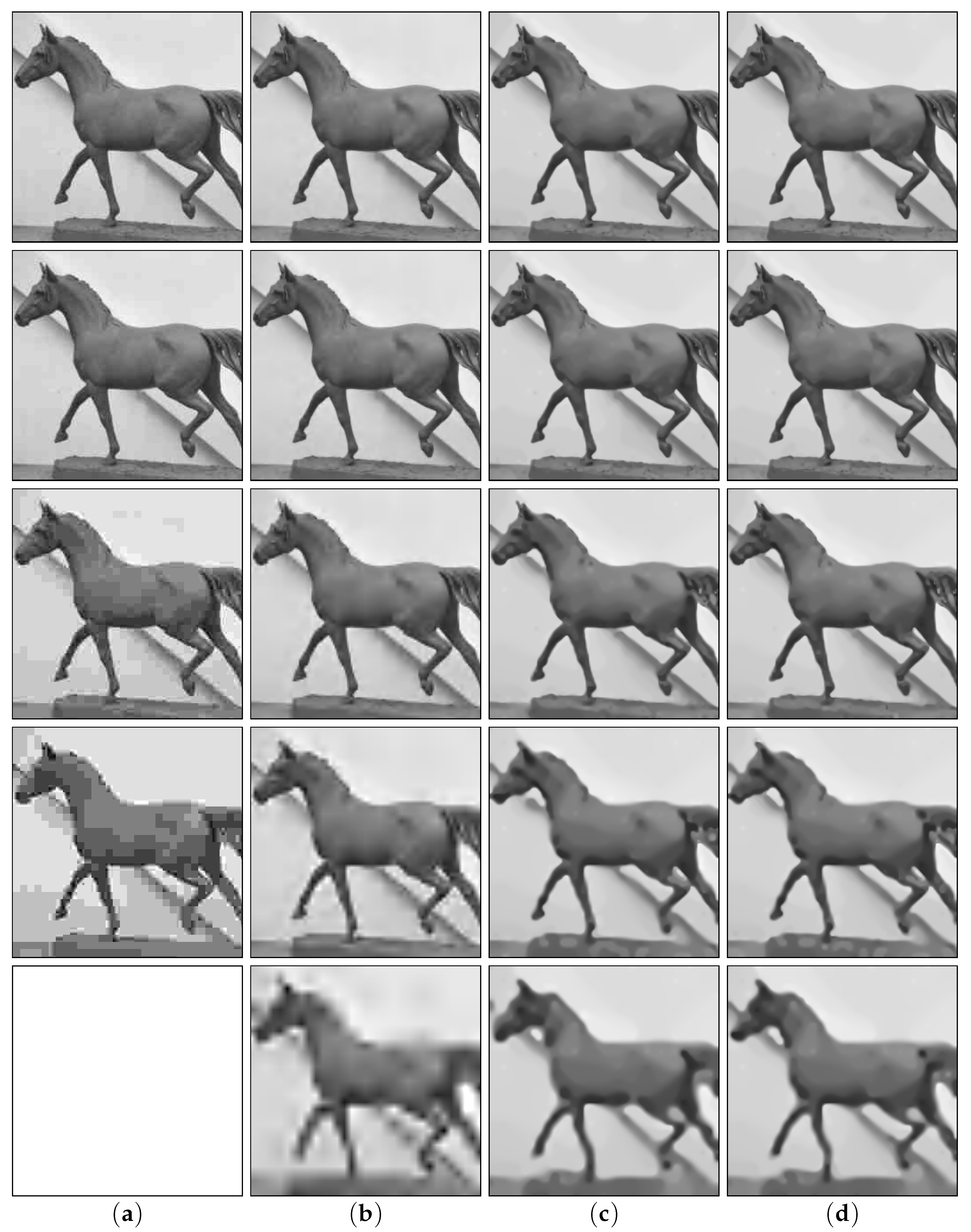
Figure 11.
Comparative overview of reconstructed images ranging from 0.8 bpp (top row) to 0.05 bpp (bottom row). Compression methods: (a) JPEG, (b) JPEG 2000, (c) EEDC i, and (d) EEDC-RANGE (BWT).
Figure 11.
Comparative overview of reconstructed images ranging from 0.8 bpp (top row) to 0.05 bpp (bottom row). Compression methods: (a) JPEG, (b) JPEG 2000, (c) EEDC i, and (d) EEDC-RANGE (BWT).
Figure 12.
A segment of the binary tree structure obtained using triangular coding.
Figure 12.
A segment of the binary tree structure obtained using triangular coding.
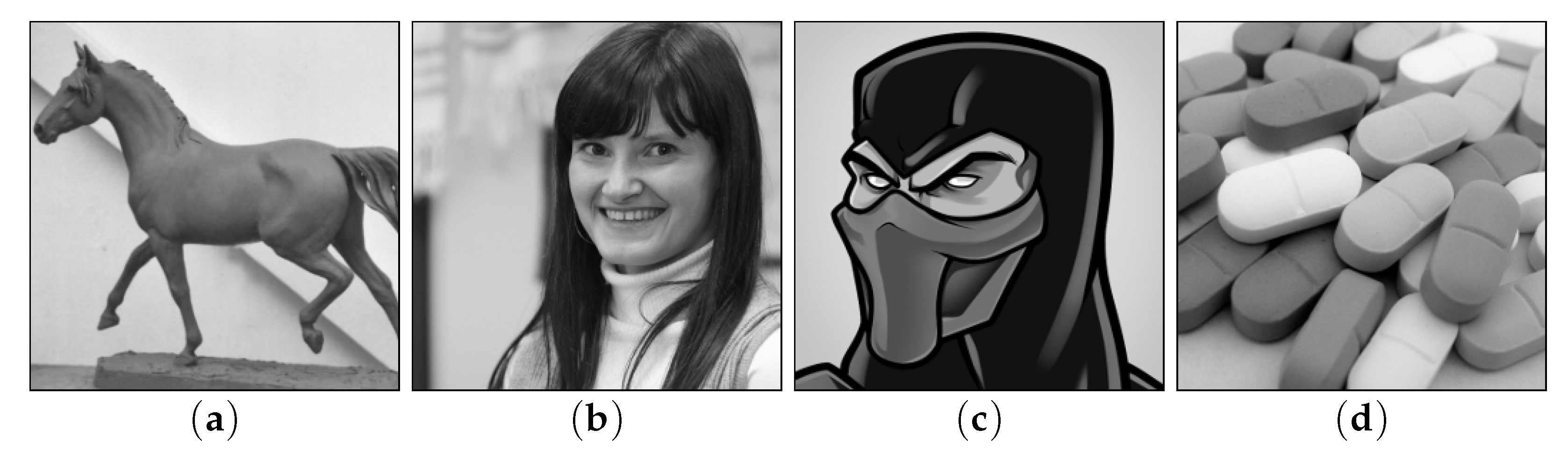
Figure 13.
Test images: (a) horse, (b) beauty, (c) mask, and (d) pills.
Figure 13.
Test images: (a) horse, (b) beauty, (c) mask, and (d) pills.
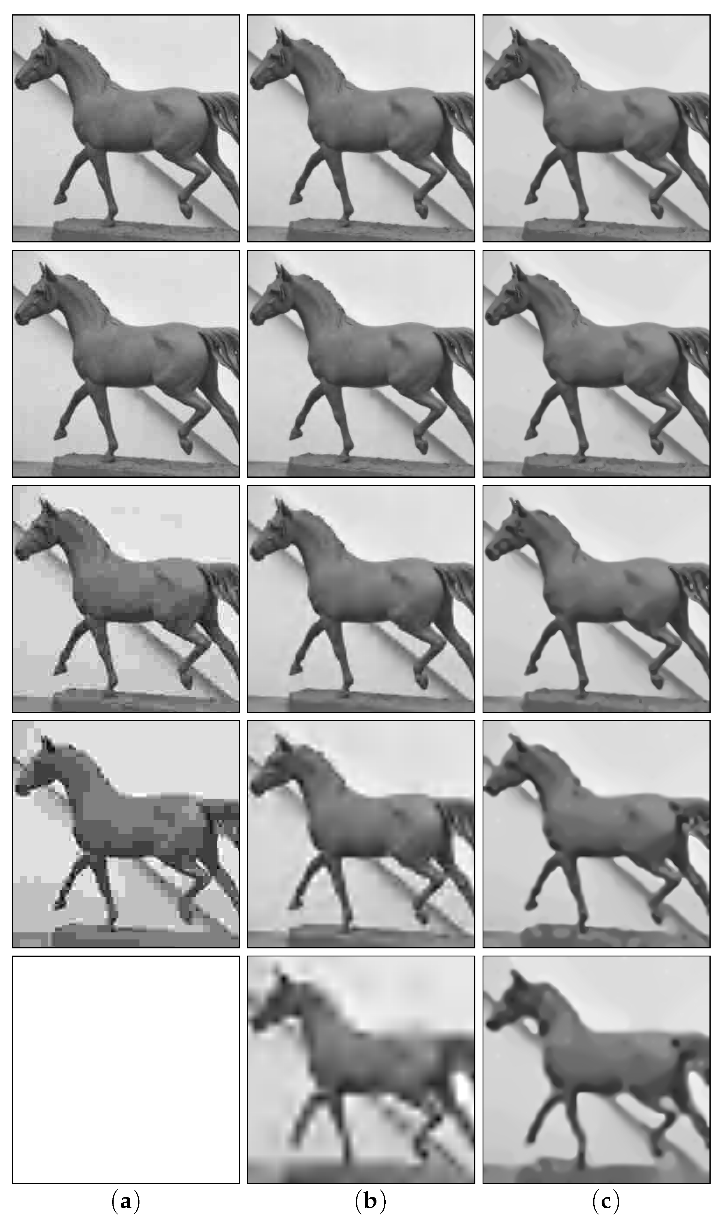
Figure 14.
Comparative overview of reconstructed images for image horse ranging from 0.8 bpp (top row) to 0.05 bpp (bottom row). Compression methods: (a) JPEG, (b) JPEG 2000, and (c) EEDC-BSSP.
Figure 14.
Comparative overview of reconstructed images for image horse ranging from 0.8 bpp (top row) to 0.05 bpp (bottom row). Compression methods: (a) JPEG, (b) JPEG 2000, and (c) EEDC-BSSP.
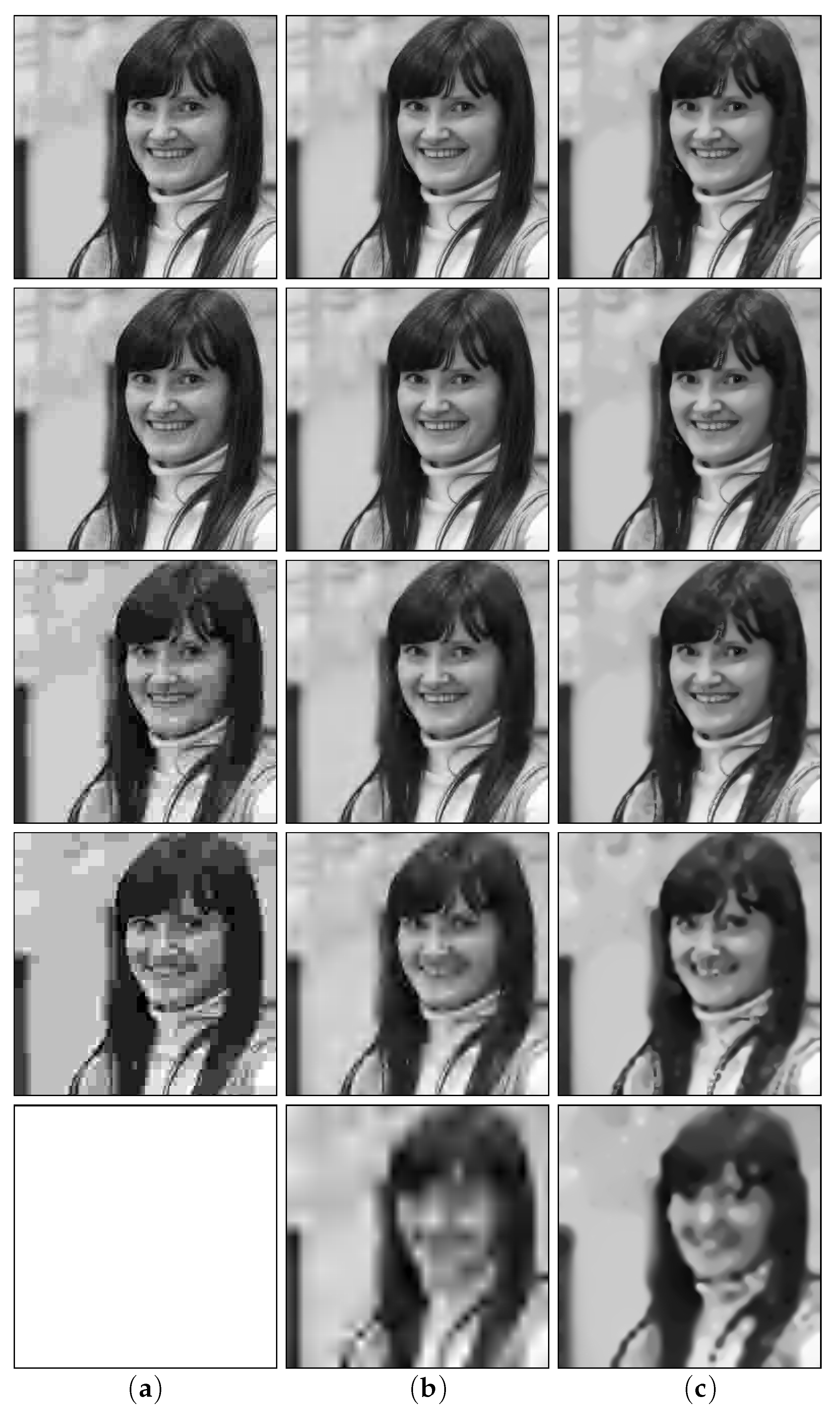
Figure 15.
Comparative overview of reconstructed images for image beauty ranging from 0.8 bpp (top row) to 0.05 bpp (bottom row). Compression methods: (a) JPEG, (b) JPEG 2000, and (c) EEDC-BSSP.
Figure 15.
Comparative overview of reconstructed images for image beauty ranging from 0.8 bpp (top row) to 0.05 bpp (bottom row). Compression methods: (a) JPEG, (b) JPEG 2000, and (c) EEDC-BSSP.
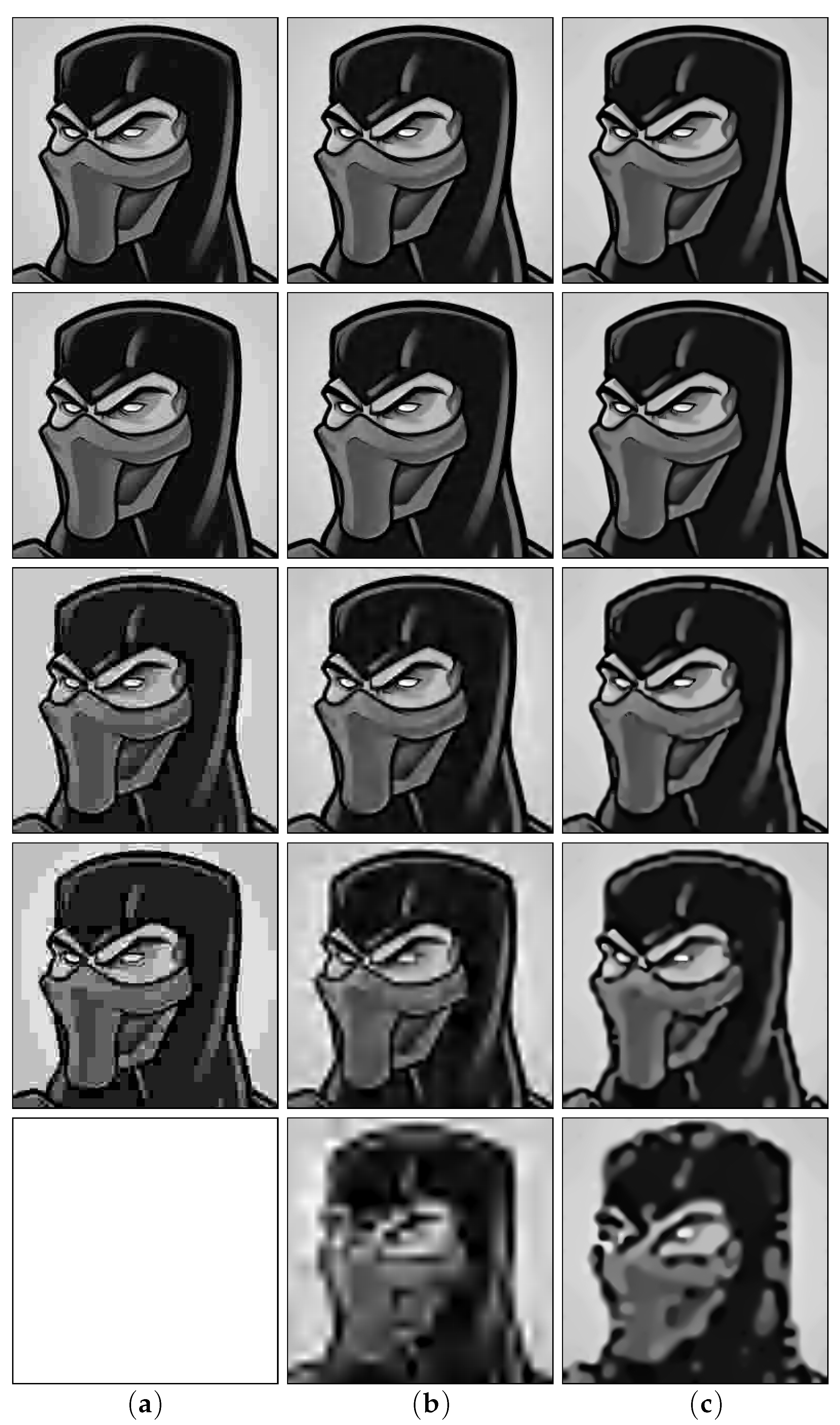
Figure 16.
Comparative overview of reconstructed images for image mask ranging from 0.8 bpp (top row) to 0.05 bpp (bottom row). Compression methods: (a) JPEG, (b) JPEG 2000, and (c) EEDC-BSSP.
Figure 16.
Comparative overview of reconstructed images for image mask ranging from 0.8 bpp (top row) to 0.05 bpp (bottom row). Compression methods: (a) JPEG, (b) JPEG 2000, and (c) EEDC-BSSP.
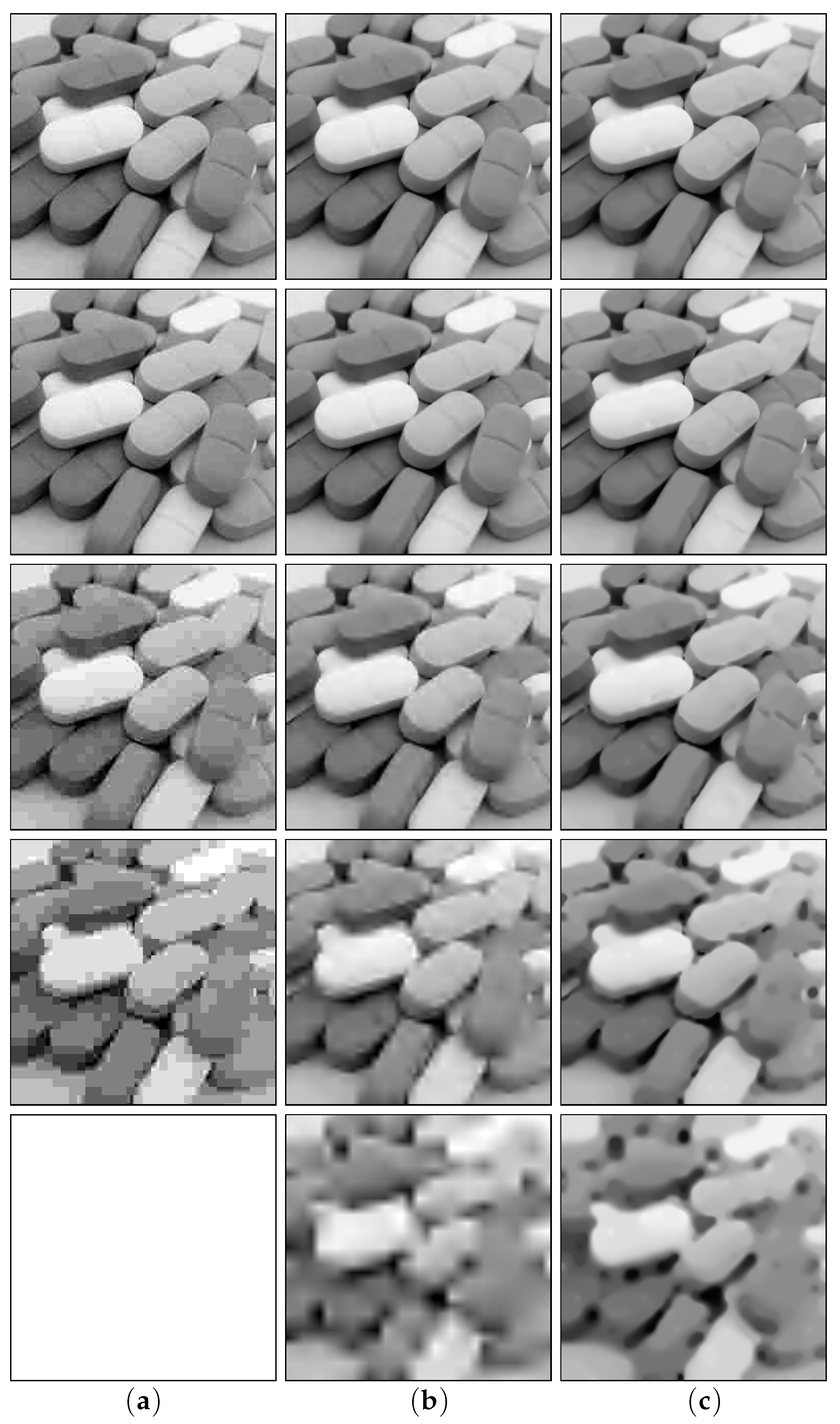
Figure 17.
Comparative overview of reconstructed images for image pills ranging from 0.8 bpp (top row) to 0.05 bpp (bottom row). Compression methods: (a) JPEG, (b) JPEG 2000, and (c) EEDC-BSSP.
Figure 17.
Comparative overview of reconstructed images for image pills ranging from 0.8 bpp (top row) to 0.05 bpp (bottom row). Compression methods: (a) JPEG, (b) JPEG 2000, and (c) EEDC-BSSP.
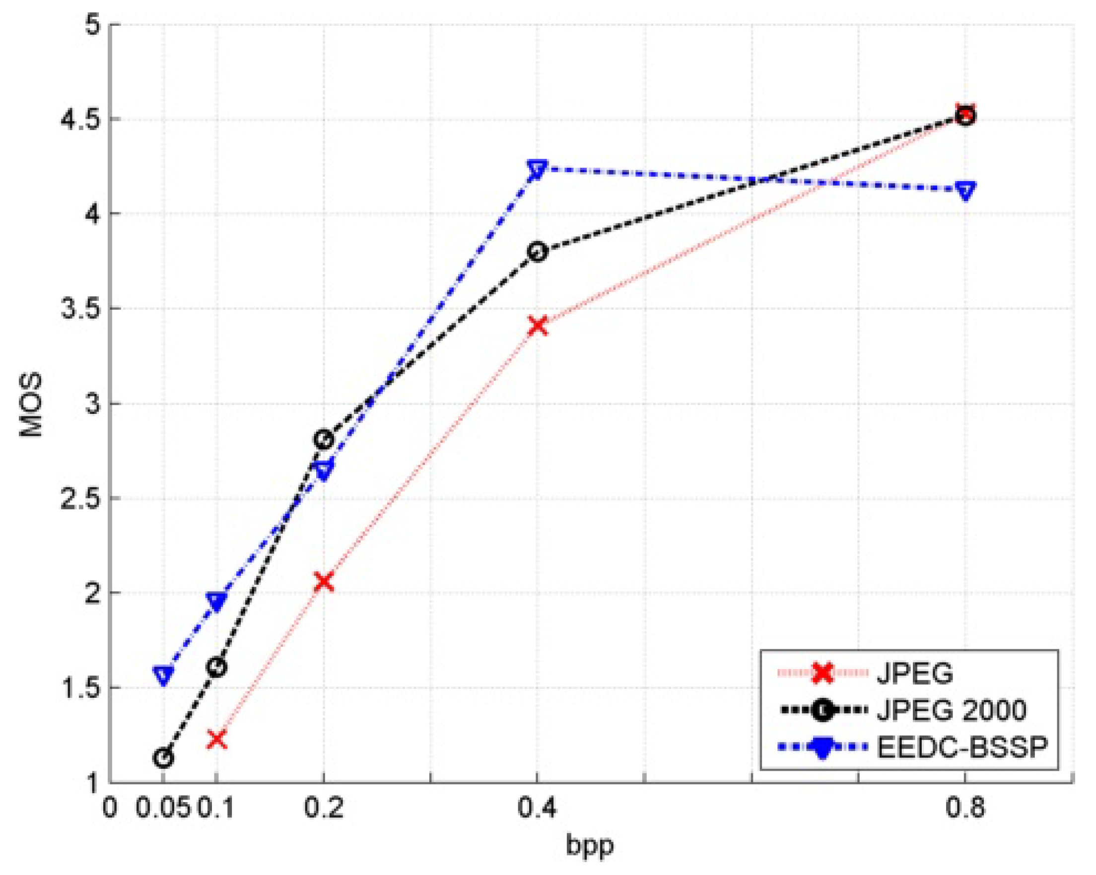
Figure 18.
MOS values comparison for EEDC-BSSP with JPEG and JPEG 2000 for image horse.
Figure 18.
MOS values comparison for EEDC-BSSP with JPEG and JPEG 2000 for image horse.
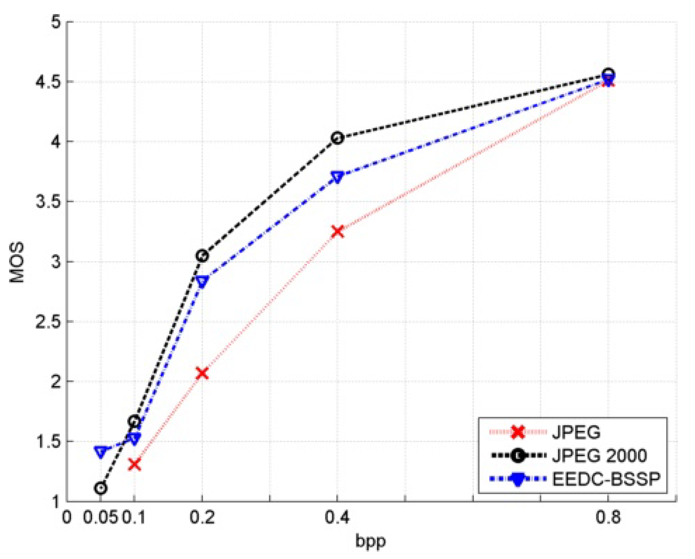
Figure 19.
MOS values comparison for EEDC-BSSP with JPEG and JPEG 2000 for image beauty.
Figure 19.
MOS values comparison for EEDC-BSSP with JPEG and JPEG 2000 for image beauty.
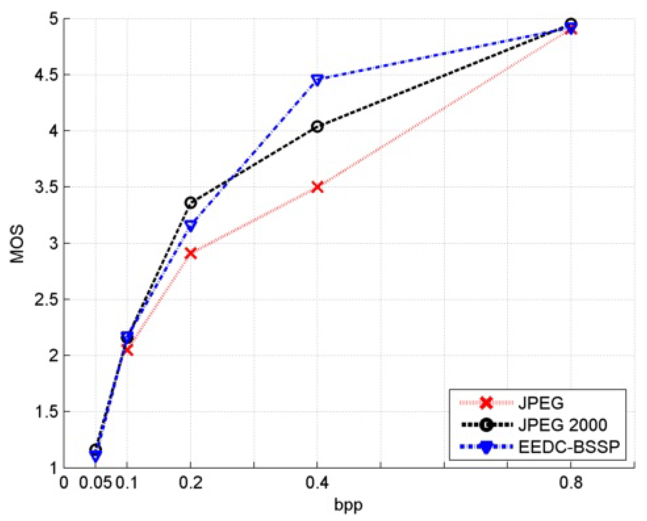
Figure 20.
MOS values comparison for EEDC-BSSP with JPEG and JPEG 2000 for image mask.
Figure 20.
MOS values comparison for EEDC-BSSP with JPEG and JPEG 2000 for image mask.
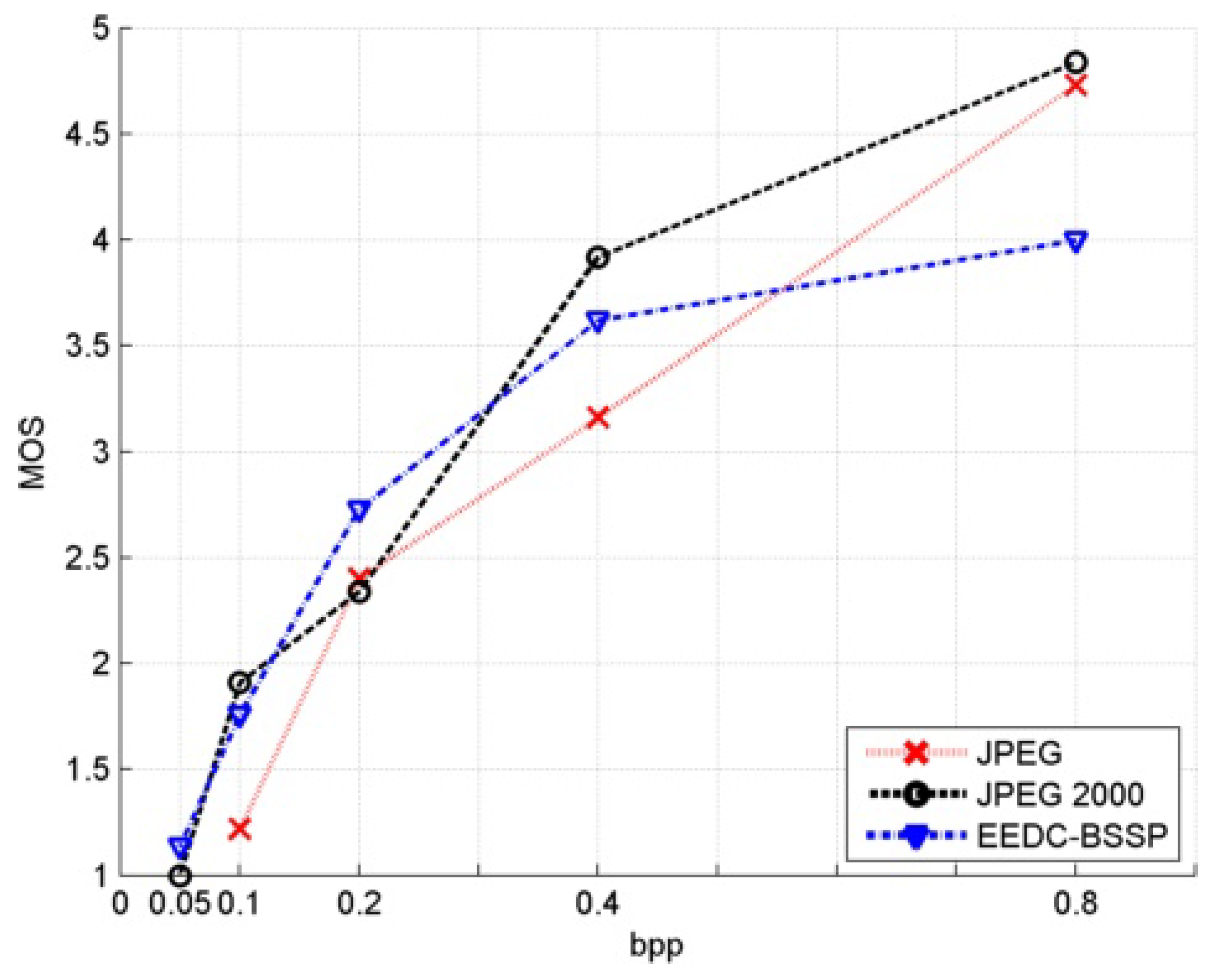
Figure 21.
MOS values comparison for EEDC-BSSP with JPEG and JPEG 2000 for image pills.
Figure 21.
MOS values comparison for EEDC-BSSP with JPEG and JPEG 2000 for image pills.
Table 1.
Average absolute error (AAE) and mean square error (MSE) for the sparse data interpolation of the image horse.
Table 1.
Average absolute error (AAE) and mean square error (MSE) for the sparse data interpolation of the image horse.
| PDE Method | AAE | MSE |
|---|
| Homogeneous diffusion | 14.98 | 366.94 |
| Biharmonic smoothing | 13.16 | 373.52 |
| Triharmonic smoothing | 16.25 | 491.15 |
| AMLE | 14.91 | 376.99 |
| Charbonnier diffusion | 18.66 | 572.03 |
| Edge-enhancing diffusion | 12.52 | 353.12 |
Table 2.
Comparison of Average Absolute Error for image horse on an unmodified compression algorithm.
Table 2.
Comparison of Average Absolute Error for image horse on an unmodified compression algorithm.
| bpp | JPEG | JPEG 2000 | EEDC |
|---|
| 0.8 | 1.65 | 1.39 | 2.08 |
| 0.4 | 2.91 | 2.29 | 2.67 |
| 0.2 | 6.20 | 3.78 | 3.80 |
| 0.1 | 10.96 | 6.75 | 5.94 |
| 0.05 | / | 12.52 | 9.31 |
Table 3.
Average absolute error for image horse and LZ-family coders.
Table 3.
Average absolute error for image horse and LZ-family coders.
| bpp | LZ77 | LZ78 | LZW |
|---|
| 0.8 | 3.01 | 3.77 | 3.62 |
| 0.4 | 3.51 | 3.92 | 3.84 |
| 0.2 | 4.33 | 4.71 | 4.58 |
| 0.1 | 7.12 | 7.90 | 7.33 |
| 0.05 | 14.22 | 15.20 | 14.78 |
Table 4.
Comparison of average absolute error for image horse and all modified compression algorithms.
Table 4.
Comparison of average absolute error for image horse and all modified compression algorithms.
| bpp | JPEG | JPEG 2000 | EEDC | EEDC-Arith | EEDC-Range | EEDC-LZ77 | EEDC-LZ78 | EEDC-LZW |
|---|
| 0.8 | 1.65 | 1.39 | 2.08 | 2.49 | 2.24 | 3.01 | 3.77 | 3.62 |
| 0.4 | 2.91 | 2.29 | 2.67 | 3.03 | 2.88 | 3.51 | 3.92 | 3.84 |
| 0.2 | 6.20 | 3.78 | 3.80 | 3.98 | 3.86 | 4.33 | 4.71 | 4.58 |
| 0.1 | 10.96 | 6.75 | 5.94 | 6.50 | 6.31 | 7.12 | 7.90 | 7.33 |
| 0.05 | / | 12.52 | 9.31 | 10.20 | 10.08 | 14.22 | 15.20 | 14.78 |
Table 5.
Possible combinations of coders and transformations.
Table 5.
Possible combinations of coders and transformations.
| Compression Method | Input Stream Transformation |
|---|
| Delta Coding | CTW | BWT | PPM | DMC |
|---|
| Huffman coding | ✓ | ✓ | ✓ | ✓ | |
| Arithmetic coding | ✓ | ✓ | ✓ | ✓ | ✓ |
| Range coding | ✓ | ✓ | ✓ | ✓ | ✓ |
| LZ77 | ✓ | | ✓ | ✓ | |
| LZ78 | ✓ | | ✓ | ✓ | |
| LZW | ✓ | | ✓ | ✓ | |
Table 6.
AAE for all possible combinations of the compression and transformation.
Table 6.
AAE for all possible combinations of the compression and transformation.
| Compression Method | Input Stream Transformation |
|---|
| Delta Coding | CTW | BWT | PPM | DMC |
|---|
| Huffman coding | 3.89 | 3.91 | 3.84 | 4.12 | / |
| Arithmetic coding | 4.02 | 3.91 | 3.88 | 4.09 | 4.53 |
| Range coding | 3.91 | 3.84 | 3.61 | 3.93 | 4.11 |
| LZ77 | 4.21 | / | 3.91 | 4.51 | / |
| LZ78 | 4.55 | / | 4.17 | 5.01 | / |
| LZW | 4.34 | / | 3.99 | 4.89 | / |
Table 7.
AAE values comparison.
Table 7.
AAE values comparison.
| bpp | JPEG | JPEG 2000 | EEDC | EEDC-RANGE (BWT) |
|---|
| 0.8 | 1.65 | 1.39 | 2.08 | 2.02 |
| 0.4 | 2.91 | 2.29 | 2.67 | 2.52 |
| 0.2 | 6.20 | 3.78 | 3.80 | 3.61 |
| 0.1 | 10.96 | 6.75 | 5.94 | 5.65 |
| 0.05 | / | 12.52 | 9.31 | 8.68 |
Table 8.
AAE for possible combinations of data transformation and compression at binary tree structure coding.
Table 8.
AAE for possible combinations of data transformation and compression at binary tree structure coding.
| Compression Method | Data Stream Transformation |
|---|
| None | Delta Coding | CTW | BWT | PPM | DMC |
|---|
| Huffman coding | 4.75 | 6.12 | 4.22 | 4.68 | 4.66 | / |
| Arithmetic coding | 5.02 | 7.10 | 4.08 | 5.11 | 4.21 | 3.80 |
| Range coding | 5.33 | 7.24 | 3.99 | 5.39 | 4.13 | 3.84 |
| LZ77 | 4.68 | 5.88 | / | 4.65 | 4.34 | / |
| LZ78 | 4.89 | 6.01 | / | 4.93 | 4.48 | / |
| LZW | 4.76 | 5.94 | / | 4.87 | 4.42 | / |
Table 9.
Results of the AAE, MSE, and SNR metrics for image horse.
Table 9.
Results of the AAE, MSE, and SNR metrics for image horse.
| bpp | AAE | MSE | SNR |
|---|
| JPEG | JPEG 2000 | EEDC BSSP | JPEG | JPEG 2000 | EEDC BSSP | JPEG | JPEG 2000 | EEDC BSSP |
|---|
| 0.8 | 1.65 | 1.39 | 1.97 | 6.51 | 3.50 | 6.22 | 27.09 | 29.88 | 27.44 |
| 0.4 | 2.91 | 2.29 | 2.45 | 19.74 | 11.15 | 11.04 | 22.28 | 24.89 | 24.91 |
| 0.2 | 6.20 | 3.78 | 3.47 | 75.08 | 36.45 | 29.00 | 16.61 | 19.66 | 20.64 |
| 0.1 | 10.96 | 6.75 | 5.46 | 231.92 | 115.60 | 88.25 | 11.57 | 14.60 | 15.82 |
| 0.05 | / | 12.52 | 8.84 | / | 353.12 | 257.27 | / | 9.47 | 11.05 |
Table 10.
Results of the PSNR, SSIM, and MS-SSIM metrics for image horse.
Table 10.
Results of the PSNR, SSIM, and MS-SSIM metrics for image horse.
| bpp | PSNR | SSIM | MS-SSIM |
|---|
| JPEG | JPEG 2000 | EEDC BSSP | JPEG | JPEG 2000 | EEDC BSSP | JPEG | JPEG 2000 | EEDC BSSP |
|---|
| 0.8 | 39.99 | 42.70 | 40.19 | 0.97 | 0.98 | 0.97 | 1.00 | 1.00 | 0.99 |
| 0.4 | 35.18 | 37.66 | 37.70 | 0.93 | 0.96 | 0.96 | 0.99 | 0.99 | 0.99 |
| 0.2 | 29.38 | 32.51 | 33.51 | 0.84 | 0.92 | 0.93 | 0.94 | 0.98 | 0.98 |
| 0.1 | 24.48 | 27.50 | 28.67 | 0.74 | 0.84 | 0.88 | 0.87 | 0.95 | 0.95 |
| 0.05 | / | 22.65 | 24.03 | / | 0.72 | 0.87 | / | 0.82 | 0.89 |
Table 11.
Results of the VIF metric for image horse.
Table 11.
Results of the VIF metric for image horse.
| bpp | JPEG | JPEG 2000 | EEDC BSSP |
|---|
| 0.8 | 0.75 | 0.80 | 0.75 |
| 0.4 | 0.59 | 0.66 | 0.67 |
| 0.2 | 0.38 | 0.50 | 0.54 |
| 0.1 | 0.23 | 0.33 | 0.38 |
| 0.05 | / | 0.17 | 0.23 |
Table 12.
Results of the AAE, MSE, and SNR metrics for image beauty.
Table 12.
Results of the AAE, MSE, and SNR metrics for image beauty.
| bpp | AAE | MSE | SNR |
|---|
| JPEG | JPEG 2000 | EEDC BSSP | JPEG | JPEG 2000 | EEDC BSSP | JPEG | JPEG 2000 | EEDC BSSP |
|---|
| 0.8 | 2.53 | 2.08 | 3.01 | 15.53 | 8.23 | 17.16 | 25.05 | 27.84 | 24.70 |
| 0.4 | 4.34 | 3.27 | 4.10 | 41.19 | 22.82 | 33.87 | 20.82 | 23.41 | 21.68 |
| 0.2 | 8.34 | 4.91 | 5.12 | 131.02 | 48.28 | 51.51 | 15.80 | 19.83 | 19.31 |
| 0.1 | 12.40 | 8.08 | 7.82 | 270.45 | 140.47 | 128.15 | 12.50 | 15.46 | 15.81 |
| 0.05 | / | 13.46 | 12.20 | / | 384.84 | 300.65 | / | 10.86 | 11.89 |
Table 13.
Results of the PSNR, SSIM, and MS-SSIM metrics for image beauty.
Table 13.
Results of the PSNR, SSIM, and MS-SSIM metrics for image beauty.
| bpp | PSNR | SSIM | MS-SSIM |
|---|
| JPEG | JPEG 2000 | EEDC BSSP | JPEG | JPEG 2000 | EEDC BSSP | JPEG | JPEG 2000 | EEDC BSSP |
|---|
| 0.8 | 36.22 | 38.98 | 35.79 | 0.95 | 0.97 | 0.94 | 0.99 | 0.99 | 0.99 |
| 0.4 | 31.98 | 34.55 | 32.83 | 0.89 | 0.93 | 0.91 | 0.98 | 0.99 | 0.98 |
| 0.2 | 26.96 | 31.01 | 30.48 | 0.76 | 0.88 | 0.87 | 0.91 | 0.97 | 0.97 |
| 0.1 | 23.81 | 26.66 | 27.05 | 0.68 | 0.79 | 0.80 | 0.85 | 0.92 | 0.93 |
| 0.05 | / | 22.28 | 23.35 | / | 0.66 | 0.73 | / | 0.78 | 0.85 |
Table 14.
Results of the VIF metric for image beauty.
Table 14.
Results of the VIF metric for image beauty.
| bpp | JPEG | JPEG 2000 | EEDC BSSP |
|---|
| 0.8 | 0.69 | 0.74 | 0.65 |
| 0.4 | 0.53 | 0.60 | 0.55 |
| 0.2 | 0.32 | 0.49 | 0.46 |
| 0.1 | 0.21 | 0.32 | 0.34 |
| 0.05 | / | 0.19 | 0.23 |
Table 15.
Results of the AAE, MSE, and SNR metrics for image mask.
Table 15.
Results of the AAE, MSE, and SNR metrics for image mask.
| bpp | PSNR | SSIM | MS-SSIM |
|---|
| JPEG | JPEG 2000 | EEDC BSSP | JPEG | JPEG 2000 | EEDC BSSP | JPEG | JPEG 2000 | EEDC BSSP |
|---|
| 0.8 | 2.53 | 2.08 | 3.01 | 15.53 | 8.23 | 17.16 | 25.05 | 27.84 | 24.70 |
| 0.4 | 4.34 | 3.27 | 4.10 | 41.19 | 22.82 | 33.87 | 20.82 | 23.41 | 21.68 |
| 0.2 | 8.34 | 4.91 | 5.12 | 131.02 | 48.28 | 51.51 | 15.80 | 19.83 | 19.31 |
| 0.1 | 12.40 | 8.08 | 7.82 | 270.45 | 140.47 | 128.15 | 12.50 | 15.46 | 15.81 |
| 0.05 | / | 13.46 | 12.20 | / | 384.84 | 300.65 | / | 10.86 | 11.89 |
Table 16.
Results of the PSNR, SSIM, and MS-SSIM metrics for image mask.
Table 16.
Results of the PSNR, SSIM, and MS-SSIM metrics for image mask.
| bpp | PSNR | SSIM | MS-SSIM |
|---|
| JPEG | JPEG 2000 | EEDC BSSP | JPEG | JPEG 2000 | EEDC BSSP | JPEG | JPEG 2000 | EEDC BSSP |
|---|
| 0.8 | 36.22 | 38.98 | 35.79 | 0.95 | 0.97 | 0.94 | 0.99 | 0.99 | 0.99 |
| 0.4 | 31.98 | 34.55 | 32.83 | 0.89 | 0.93 | 0.91 | 0.98 | 0.99 | 0.98 |
| 0.2 | 26.96 | 31.01 | 30.48 | 0.76 | 0.88 | 0.87 | 0.91 | 0.97 | 0.97 |
| 0.1 | 23.81 | 26.66 | 27.05 | 0.68 | 0.79 | 0.80 | 0.85 | 0.92 | 0.93 |
| 0.05 | / | 22.28 | 23.35 | / | 0.66 | 0.73 | / | 0.78 | 0.85 |
Table 17.
Results of the VIF metric for image mask.
Table 17.
Results of the VIF metric for image mask.
| bpp | JPEG | JPEG 2000 | EEDC BSSP |
|---|
| 0.8 | 0.69 | 0.74 | 0.65 |
| 0.4 | 0.53 | 0.60 | 0.55 |
| 0.2 | 0.32 | 0.49 | 0.46 |
| 0.1 | 0.21 | 0.32 | 0.34 |
| 0.05 | / | 0.19 | 0.23 |
Table 18.
Results of the AAE, MSE, and SNR metrics for image pills.
Table 18.
Results of the AAE, MSE, and SNR metrics for image pills.
| bpp | PSNR | SSIM | MS-SSIM |
|---|
| JPEG | JPEG 2000 | EEDC BSSP | JPEG | JPEG 2000 | EEDC BSSP | JPEG | JPEG 2000 | EEDC BSSP |
|---|
| 0.8 | 1.75 | 1.48 | 1.92 | 6.55 | 3.95 | 5.98 | 26.15 | 28.44 | 26.67 |
| 0.4 | 3.29 | 2.47 | 2.59 | 22.05 | 12.19 | 12.40 | 20.88 | 23.56 | 23.41 |
| 0.2 | 6.17 | 4.25 | 4.19 | 72.37 | 39.12 | 38.71 | 15.74 | 18.41 | 18.46 |
| 0.1 | 11.94 | 7.23 | 6.51 | 243.65 | 114.56 | 102.60 | 10.55 | 13.68 | 14.13 |
| 0.05 | / | 13.34 | 10.29 | / | 362.35 | 257.54 | / | 8.20 | 9.92 |
Table 19.
Results of the PSNR, SSIM, and MS-SSIM metrics for image pills.
Table 19.
Results of the PSNR, SSIM, and MS-SSIM metrics for image pills.
| bpp | PSNR | SSIM | MS-SSIM |
|---|
| JPEG | JPEG 2000 | EEDC BSSP | JPEG | JPEG 2000 | EEDC BSSP | JPEG | JPEG 2000 | EEDC BSSP |
|---|
| 0.8 | 39.97 | 42.17 | 40.36 | 0.97 | 0.98 | 0.97 | 1.00 | 1.00 | 0.99 |
| 0.4 | 34.70 | 37.27 | 37.20 | 0.92 | 0.96 | 0.96 | 0.98 | 0.99 | 0.99 |
| 0.2 | 29.54 | 32.21 | 32.25 | 0.82 | 0.90 | 0.92 | 0.94 | 0.97 | 0.97 |
| 0.1 | 24.26 | 27.54 | 28.02 | 0.68 | 0.82 | 0.85 | 0.84 | 0.93 | 0.94 |
| 0.05 | / | 22.54 | 24.02 | / | 0.69 | 0.76 | / | 0.77 | 0.86 |
Table 20.
Results of the VIF metric for image pills.
Table 20.
Results of the VIF metric for image pills.
| bpp | JPEG | JPEG 2000 | EEDC BSSP |
|---|
| 0.8 | 0.76 | 0.81 | 0.77 |
| 0.4 | 0.59 | 0.68 | 0.68 |
| 0.2 | 0.39 | 0.50 | 0.52 |
| 0.1 | 0.21 | 0.34 | 0.37 |
| 0.05 | / | 0.18 | 0.24 |
Table 21.
Image distortion ratings.
Table 21.
Image distortion ratings.
| Rating | Distortion |
|---|
| 1 | Particularly irritating |
| 2 | Irritating |
| 3 | Slightly irritating |
| 4 | Noticeably |
| 5 | Not noticeably |
Table 22.
Image quality ratings.
Table 22.
Image quality ratings.
| Rating | Quality |
|---|
| 1 | Unwatchable |
| 2 | Barely watchable |
| 3 | Watchable |
| 4 | Good |
| 5 | Excellent |
Table 23.
MOS values for image horse at various compression ratios.
Table 23.
MOS values for image horse at various compression ratios.
| bpp | JPEG | JPEG 2000 | EEDC BSSP |
|---|
| 0.8 | 4.53 | 4.52 | 4.13 |
| 0.4 | 3.41 | 3.80 | 4.24 |
| 0.2 | 2.06 | 2.81 | 2.65 |
| 0.1 | 1.23 | 1.61 | 1.96 |
| 0.05 | / | 1.13 | 1.57 |
Table 24.
MOS values for image beauty at various compression ratios.
Table 24.
MOS values for image beauty at various compression ratios.
| bpp | JPEG | JPEG 2000 | EEDC BSSP |
|---|
| 0.8 | 4.51 | 4.56 | 4.52 |
| 0.4 | 3.25 | 4.03 | 3.71 |
| 0.2 | 2.07 | 3.05 | 2.84 |
| 0.1 | 1.31 | 1.67 | 1.53 |
| 0.05 | / | 1.11 | 1.42 |
Table 25.
MOS values for image mask at various compression ratios.
Table 25.
MOS values for image mask at various compression ratios.
| bpp | JPEG | JPEG 2000 | EEDC BSSP |
|---|
| 0.8 | 4.91 | 4.95 | 4.92 |
| 0.4 | 3.50 | 4.04 | 4.46 |
| 0.2 | 2.91 | 3.36 | 3.16 |
| 0.1 | 2.05 | 2.16 | 2.17 |
| 0.05 | / | 1.16 | 1.11 |
Table 26.
MOS values for image pills at various compression ratios.
Table 26.
MOS values for image pills at various compression ratios.
| bpp | JPEG | JPEG 2000 | EEDC BSSP |
|---|
| 0.8 | 4.73 | 4.84 | 4.00 |
| 0.4 | 3.16 | 3.92 | 3.62 |
| 0.2 | 2.40 | 2.34 | 2.73 |
| 0.1 | 1.22 | 1.91 | 1.76 |
| 0.05 | / | 1.00 | 1.14 |


