Review: A Survey on Objective Evaluation of Image Sharpness

Abstract

Establishing an accurate objective evaluation metric of image sharpness is crucial for image analysis, recognition and quality measurement. In this review, we highlight recent advances in no-reference image quality assessment research, divide the reported algorithms into four groups (spatial domain-based methods, spectral domain-based methods, learning-based methods and combination methods) and outline the advantages and disadvantages of each method group. Furthermore, we conduct a brief bibliometric study with which to provide an overview of the current trends from 2013 to 2021 and compare the performance of representative algorithms on public datasets. Finally, we describe the shortcomings and future challenges in the current studies.

1. Introduction

In the overview of image quality evaluation, the common evaluation indicators [1] include image noise, image color, artifacts, sharpness, etc. Image noise evaluation methods [2] mainly rely on image spatial and temporal noise, signal-to-noise ratio and grayscale noise to obtain evaluation results. The image color evaluation methods [3] usually evaluate the color degree and uniformity of the image. The image artifact evaluation methods [4] pay more attention to chromatic aberration, distortion and vignetting factors, while the image sharpness evaluation method [5] is based on the comprehensive evaluation of the edges and details of the image, which is currently one of the most popular image quality evaluation methods; it is closely related to research fields such as bionics [6], nonwoven materials [7], medicine [8], etc.

According to the dependence on the reference image, the evaluation methods are divided into three types: Full-Reference (FR), Reduced-Reference (RR) and No-Reference (NR) [9]. The FR method uses the distorted image and the corresponding undistorted reference image to generate the image quality score. In the RR method, the image quality is evaluated on partial information extracted using feature extraction methods. Unlike the FR and RR methods, the NR method can use the distorted image alone to complete the quality assessment. Since it is usually impossible to obtain an undistorted image for reference in practical applications, the research on NR methods has become the current mainstream research direction [10,11].

The image sharpness refers to the clarity of the texture and borders of various detailed parts of an image, which affects the perception of information, image acquisition, and subsequent processing, especially in some applications based on high-quality images [12,13,14]. The ideal image sharpness evaluation function should have the characteristics of high sensitivity, good robustness and low computational cost [15,16,17]. Most traditional image sharpness evaluation methods [18] are based on spatial or spectral domains. The methods in the spatial domain mainly evaluate the image by extracting the image gradient and edge information [19,20], which have the advantages of simple calculation and high real-time performance but are easily disturbed by noise. The methods in the spectral domain mainly use transformation methods, such as Fourier transform and wavelet transform, to extract image frequency features for sharpness evaluation [21]. This type of method has excellent sensitivity but high computational complexity. In recent years, learning-based methods have emerged from the machine learning methods to the deep learning methods [22]. At the same time, an increasing number of evaluation methods of a combination of methods are studied and developed by scholars. A combination method is usually a new method formed by combining two or more single evaluation methods in a certain relationship. Such methods incorporate the advantages of the single method being combined and effectively improve the accuracy of quality evaluation.

Although the above-reported research has obtained fruitful results, the objective evaluation standards for image sharpness are still not mature enough; few evaluation methods are suitable for most scenarios. It is unrealistic to ask one sharpness evaluation algorithm to handle all potential images due to the sophisticated and various image textures and features [23]. Therefore, this paper reviews and clusters the existing sharpness evaluation methods and conducted systematic comparative analyses on several representative methods aimed at offering directions for researchers to choose or develop a sharpness evaluation algorithm on different types of images.

The paper reviews, classifies and summarizes the past decade’s sharpness evaluation methods for no-reference images. The reviewed evaluation methods are grouped into four categories with their evaluation results compared and the advantages and disadvantages discussed. An outlook on the application of image sharpness in image processing is given, and a direction for further research on sharpness evaluation methods for no-reference images is discussed. Section 1 presents the background of the evaluation method. Section 2 summarizes the current sharpness evaluation methods by characterizing them into four groups. Section 3 offers a bibliometric study to evaluate and compare the performance of state-of-the-art algorithms on public datasets. Section 4 highlights the shortcomings of current research and provides an outlook on future challenges.

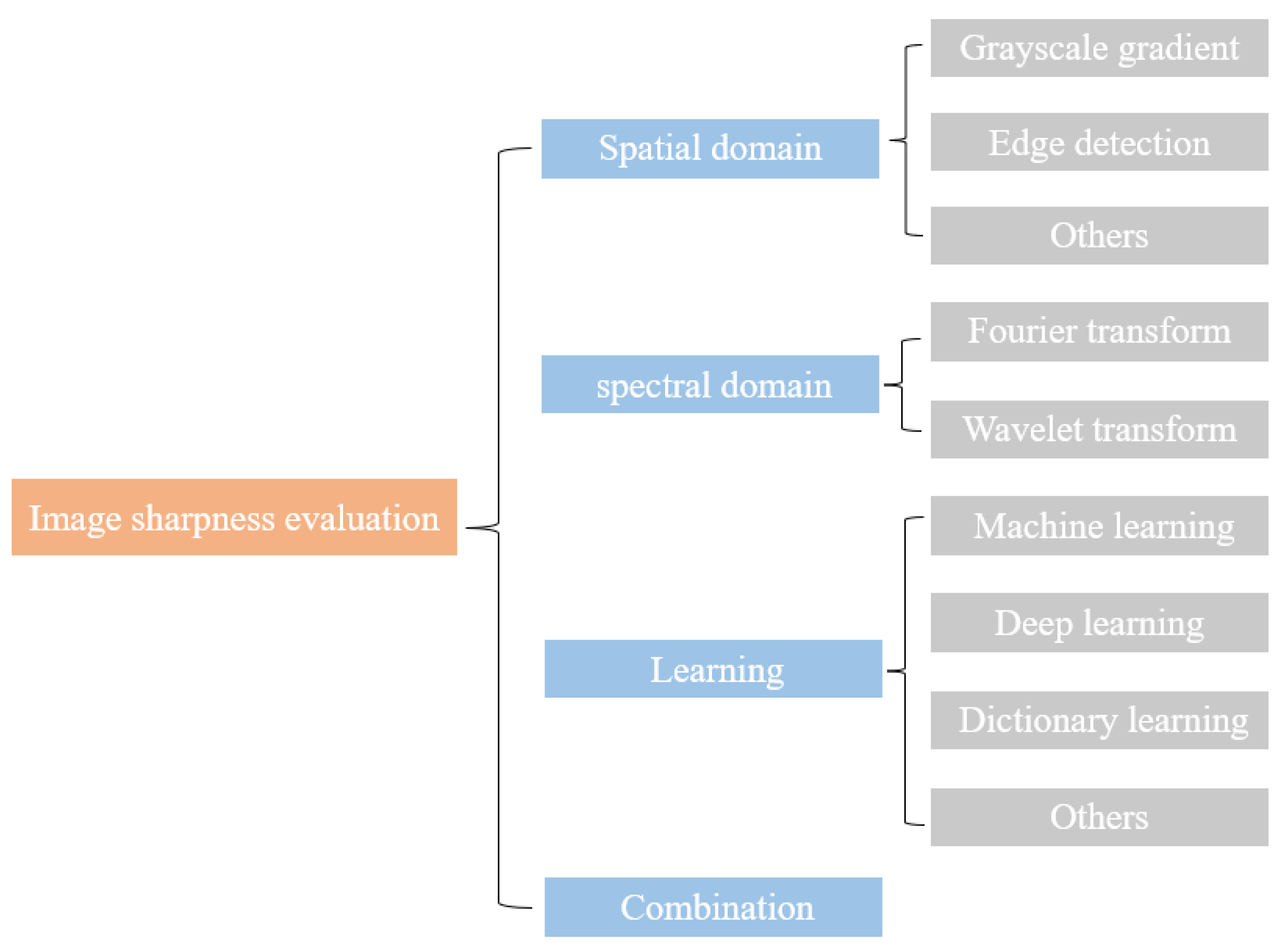
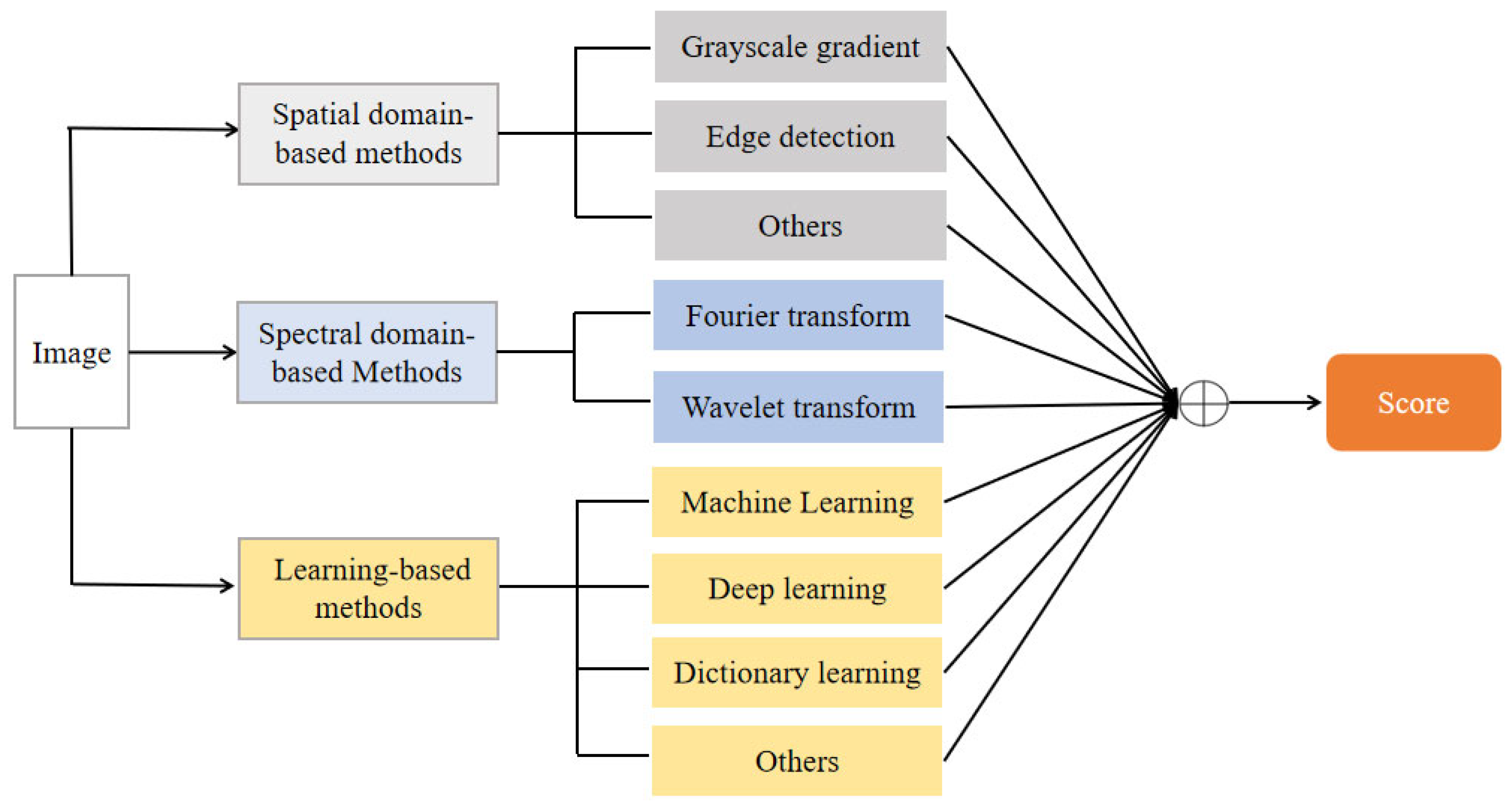
2. Evaluation Methods and Analysis

The sharpness evaluation methods for no-reference images can be divided into four categories: spatial domain methods, spectral domain methods, learning methods and combination methods. The specific classification is shown in Figure 1.

2.1. Spatial Domain-Based Methods

Early work [24,25,26] on the sharpness evaluation of no-reference images was mainly performed in the spatial domain. The spatial domain evaluation functions use the characteristics of the image in the spatial domain to distinguish between blurred and clear images [27]. This type of evaluation function generally evaluates images directly by calculating the relationship between image pixels and their neighbors. We mainly divide spatial domain methods into gradient grayscale and edge detection evaluation methods.

2.1.1. Grayscale Gradient-Based Methods

Grayscale gradient function is one of the commonly used image sharpness evaluation functions, which mainly evaluates by calculating the difference between adjacent pixels on the image to establish the evaluation function [28,29]. Classical methods include the Brenner function [30], the energy gradient function [31], Laplacian function [32], Tenengrad function [33] and so on. In addition to the classical evaluation methods based on gray gradient mentioned above, other novel methods have also been studied. Zhan et al. [34] used the maximum gradient and the variability of gradients to predict the quality of blurry images in a highly consistent way with subjective scoring. Li et al. [35] proposed a blur evaluation algorithm for no-reference images based on discrete orthogonal moments, where gradient images are divided into equal-sized blocks and orthogonal moments are calculated to characterize the image shape and obtain sharpness metrics. Zhang et al. [36] evaluated the edge sharpness by calculating the grayscale values of the eight directions of the pixels.

Most of the grayscale gradient-based methods are less computationally intensive and have high real-time performance but are susceptible to noise interference, which affects the accuracy of the evaluation.

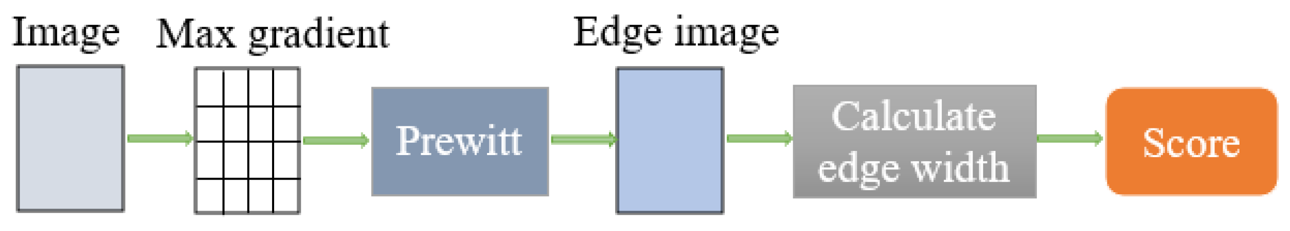
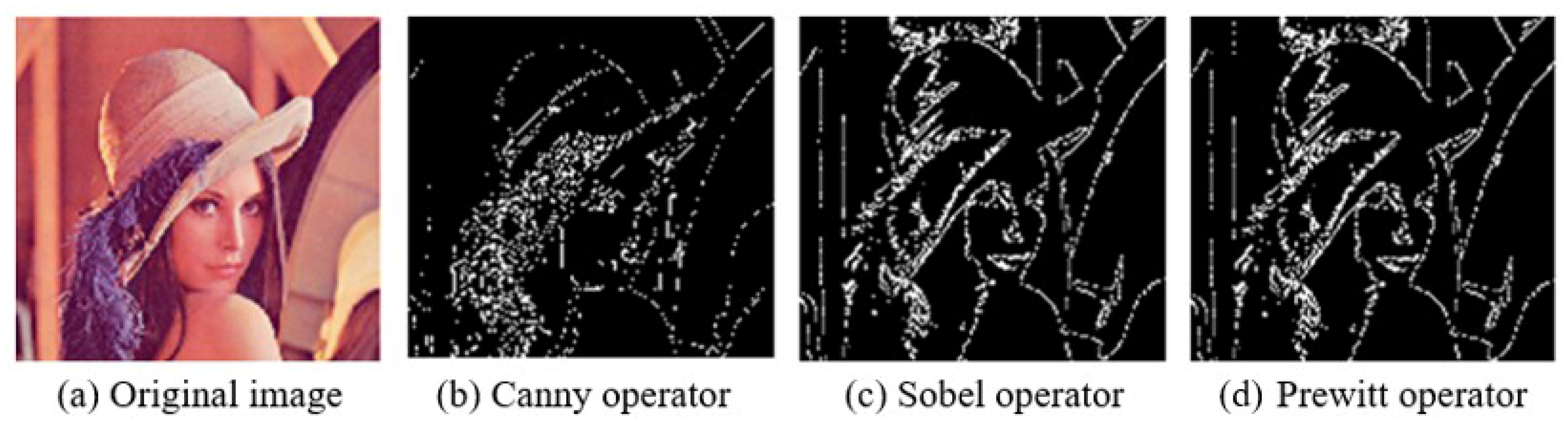
2.1.2. Edge Detection-Based Methods

The image edge is the most basic feature of an image, which refers to the discontinuity of the local characteristics of the image [37,38]. Among the edge detection-based methods, the most widely used algorithms are Canny operator [39], Sobel operator [40], Prewitt operator [41] et al.

The Canny operator is a multi-level edge detection algorithm. The Sobel operator combines Gaussian smoothing and differential derivatives to detect the horizontal and vertical edges. The Prewitt operator uses the difference generated by the grayscale values of pixels in a specific region to achieve edge detection. The process of image sharpness evaluation based on the Prewitt operator is shown in Figure 2.

As shown in Figure 3, an image is plotted with the results of the Canny operator, the Sobel operator and the Prewitt operator, respectively.

Marziliano et al. [42] proposed a method to detect the edges of an image using the Sobel operator and utilized the image edge width as the sharpness evaluation score. Zhang et al. [43] proposed an image-filtering evaluation method based on the Sobel operator and image entropy. Liu et al. [44] used the Canny edge detection algorithm based on the activation mechanism to obtain the image edge position and direction, established the histogram of edge width and obtained the sharpness evaluation metric by weighting the average edge width. The method was proven to have good accuracy and predictive monotonicity. Chen et al. [45] used the Prewitt operator and the Gabor filter to calculate the average gradient of the image to predict the local sharpness value of a fabric surface image.

Among the edge detection-based methods, the Canny operator, the Sobel operator and the Prewitt operator are widely used, and each of these operators has its own advantages. The Canny operator is sensitive to weak edges but computationally intensive; the Sobel operator is fast but susceptible to noise interference; the Prewitt operator is better at extracting the edges of images disturbed by neighboring pixels.

2.1.3. Other Methods Based on Spatial Domain

Bahrami et al. [46] obtained the quality score by calculating the maximum local variation (MLV) of image pixels. The standard deviation of the weighted MLV distribution was used as a metric to measure sharpness. The study shows that this method is characterized by high real-time performance. Gu et al. [47] developed a sharpness model by analyzing the autoregressive (AR) model parameters point-by-point to calculate the energy and contrast differences in the locally estimated AR coefficients and then quantified the image sharpness using a percentile pool to predict the overall score. This evaluation method that calculates local contrast and energy based on a mathematical model is also a spatial domain method. Chang et al. [48] proposed a new independent feature similarity index to evaluate the sharpness by calculating the structure and texture differences between two images. Niranjan et al. [49] presented a no-reference image blur metric based on the study of human blur perception for varying contrast values. The method gathered information by estimating the probability of detecting blurring at each edge in the image and then calculated the cumulative probability of blur detection to obtain the evaluation result. Lin et al. [50] proposed an adaptive definition evaluation algorithm, which achieved a better evaluation effect than the standard adaptive definition algorithm. Zhang et al. [51] presented a no-reference image quality evaluation metric based on Cartoon Texture Decomposition (CTD). Using the characteristics of CTD, the image was separated into cartoon parts with prominent edges and texture parts with noise. Then the ambiguity and noise levels were estimated respectively to predict the results.

The spatial domain-based methods require less computation, but the above methods rely much on the details of the image and are easily affected by noise.

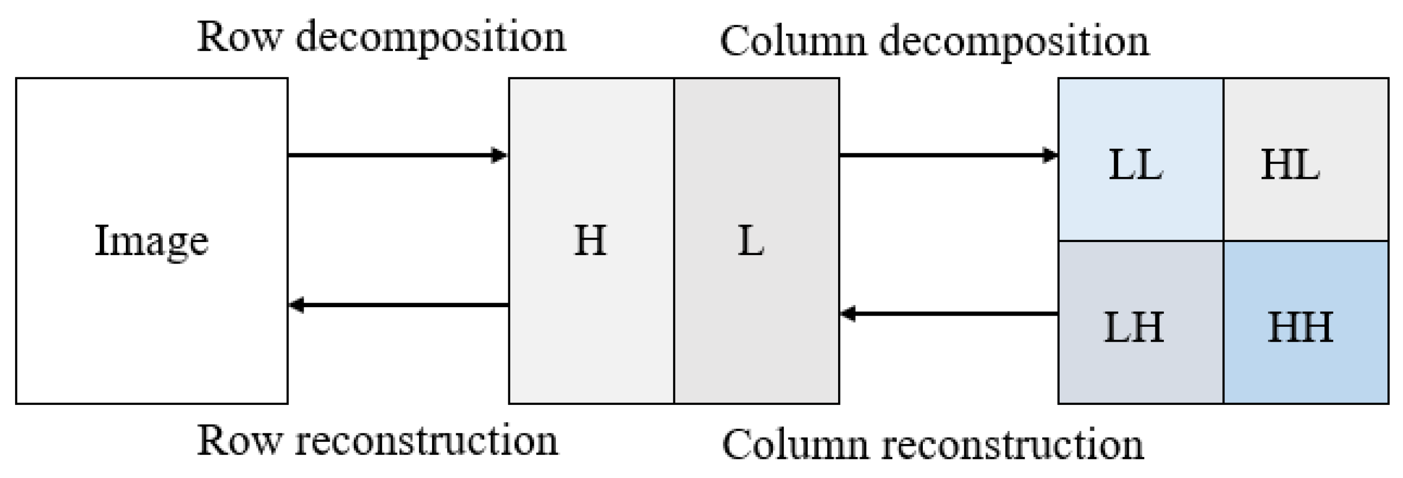
2.2. Spectral Domain-Based Methods

Frequency is an indicator that characterizes the intensity of grayscale changes in the image [52]. In spectral domain evaluation functions, the high-frequency and low-frequency components of the image correspond to sharp and blurred parts, respectively. The sharper the image, the more detail and edge information it contains. Therefore, image sharpness can be assessed by a high–low transformation in spectral domain [53]. This type of evaluation methods are usually based on Fourier transform (FT) [54], wavelet transform (WT) [55] methods, etc. The general framework of spectral domain-based methods is shown in Figure 4, where H and L represent the high-pass filter and the low-pass filter, respectively, and LL, HL, LH and HH are the corresponding components after filtering again.

2.2.1. Fourier Transform-Based Methods

The physical meaning of the Fourier transform is to convert the gray distribution function of an image into a frequency distribution function, while the inverse transform is to convert the frequency distribution function of an image into a gray distribution function [56]. Fast Fourier transform (FFT), discrete Fourier transform (DFT) and discrete cosine transform (DCT) [57] are common forms based on Fourier transform.

Kanjar et al. [58] utilized the Fourier transform spectrum to simulate the uniform blurring of Gaussian blurred images and fixed the threshold of high-frequency components for image sharpness assessment. In a related study, Kanjar et al. [59] presented a new image sharpness measure that used Discrete Cosine Transform (DCT) coefficient-based features for generating the model of image sharpness assessment. Bae et al. [60] presented a novel DCT-based Quality Degradation Metric, called DCT-QM, which was based on the probability summation theory. Bae et al. [61] also proposed a visual quality assessment method that characterized local image features and various distortion types. The visual quality perception characteristics of HVS for local image features and various distortion types are characterized by adopting Structural Contrast Index (SCI) and DCT blocks. Baig et al. [62] proposed a no-reference image quality assessment method based on the Discrete Fourier transform (DFT), calculated the image block-based DFT and averaged it at the block level and then combined them to obtain a clear metric for estimating the overall image perception quality.

The Fourier transform, as one of the most basic time-frequency transforms, can convert the image from the spatial domain to the spectral domain, synthesizing the multi-scale features but also increasing the computational effort.

2.2.2. Wavelet Transform-Based Methods

The wavelet transform method can obtain the evaluation results by using the localization characteristics of the image, and its process is shown in Figure 5, which is more suitable for the global or local evaluation of the image. In Figure 5, H and L represent the high-pass filter and the low-pass filter, respectively. The high-pass filter and the low-pass filter are used to extract edge features and image approximation, respectively.

Kerouh et al. [63] proposed a no-reference blur image evaluation method based on the wavelet transform, which extracts the high-frequency components of the image and obtains edge-defined evaluation results by analyzing multi-resolution decomposition. Vu et al. [64] presented a global and local sharpness evaluation algorithm based on fast wavelet, which decomposes the image through a three-level separable discrete wavelet transform and calculates the logarithmic energy of wavelet sub-bands for obtaining the sharpness of the image. Hassen et al. [65] proposed a method to evaluate the image sharpness of strong local phase coherence near different image features based on complex wavelet transform. Gvozden et al. [66] proposed a fast blind image sharpness/ambiguity evaluation model (BISHARP). The local contrast information of the image was obtained by calculating the root mean square of the image. At the same time, the diagonal wavelet coefficients in the wavelet transform were used for ranking and weighting to obtain the final evaluation result. Wang et al. [55] proposed a no-reference stereo image quality assessment model based on quaternion wavelet transform (QWT), which extracted a series of quality-aware features in QWT and MSCN coefficients of high-frequency sub-bands and finally predicted the sharpness score.

The spectral domain-based methods decompose the image into high-frequency and low-frequency components or sub-images of different resolution layers. They then use different functions to process these sub-images so that complex edge information can be extracted more clearly. However, the spectral domain-based methods require converting image information from the spatial domain to the spectral domain, which greatly increases the computational complexity.

The advantages and disadvantages of the different methods based on the spatial domain/spectral domain are shown in

Table 1. Advantages and disadvantages of different methods based on spatial/spectral domain.

Methods	Advantages	Disadvantages
Grayscale gradient-based methods	Simple and fast calculation	Rely on image edge information
Edge detection-based methods	High sensitivity	Susceptible to noise
Fourier transform-based methods	Extract edge features clearly	High computational complexity
Wavelet transform-based methods	High accuracy and robustness	High computational complexity and poor real-time performance

.

2.3. Learning-Based Methods

Unlike traditional methods, learning-based methods [67] can improve the accuracy of the evaluation results by learning the training image features and achieving the mapping of quality scores. The general framework of learning-based methods is shown in Figure 6. The methods can be divided into SVM-based, deep learning-based and dictionary-based methods.

2.3.1. Machine Learning-Based Methods

Early learning-based sharpness evaluation methods [68,69] for no-reference images are mainly supported vector machine (SVM) models based on machine learning, including support vector regression (SVR)/support vector clustering (SVC) methods.

Pei et al. [70] presented a sharpness evaluation method of no-reference images based on large-scale structures. The statistical scale of edges with different widths and the average value of the maximum gradient were taken as the image features, and the SVR is used to obtain the features to obtain the evaluation results. This method can avoid the interference of small textures and contrast around the edge to the evaluation results. Liu et al. [71] used the anisotropy of the orientation selectivity mechanism and the influence of gradient orientation effect on vision to extract structural information and then used Toggle operator to extract edge information as the weight of local patterns. Finally, support vector regression (SVR) was used to train prediction models with optimization characteristics and subjective scores. Moorthy et al. [72] proposed a new two-step framework for no-reference image quality assessment based on natural scene statistics (NSS). SVM is used to classify the distortion types of the fitted parameter features, and then SVR is used to calculate the image quality evaluation results under different distortion types.

Machine learning-based evaluation methods can achieve better results than other algorithms on small-sample training sets, but the extracted features determine the quality of the evaluation results.

2.3.2. Deep Learning-Based Methods

An increasing number of related deep learning methods are applied to image sharpness evaluation with the continuous improvement of deep learning methods [73]. The deep learning-based methods do not need to extract features manually but directly build a deep learning model and obtain the evaluation score of the image after training. These types of methods include a variety of network models, and nowadays, there are convolutional neural network (CNN), deep convolutional neural network (DCNN), generative adversarial network (GAN), etc. Such methods enable the learning of image quality prediction networks.

Zhu et al. [74] evaluated image quality by a method based on an optimized convolutional neural network structure, aiming to automatically extract distinctive image quality features, to improve the network learning ability and to predict the evaluation score through normalization and packet loss. Li et al. [75] divided the entire image into blocks and then used a deep convolutional neural network (DCNN) to extract their advanced features. They then aggregated information from different blocks and fed these aggregated features into a least-squares regression model to obtain sharpness evaluation values. Lin et al. [76] proposed the generation of a pseudo-reference image from the distorted image first, then paired the information of the pseudo-reference image with the distorted images and input them into the quality regression network to obtain the quality prediction result. Zhang et al. [77] proposed a deep bilinear model for blind image quality assessment (BIQA) that works for both synthetically and authentically distorted images and is able to predict image quality values. Bianco et al. [78] used the features extracted by the pre-trained convolutional neural network (CNN) as the general image description and estimated the overall image score by averaging the predicted scores in multiple sub-regions of the original image. Gao et al. [79] extracted multi-level representations of images from VGGNet (Visual Geometry Group Net), calculated a feature on each layer, then estimated the quality score of each feature vector and finally obtained the final evaluation result by averaging.

Deep learning-based methods can automatically learn multi-layer representations of image features from large amounts of data to obtain image feature information for image quality assessment, but their network models are only applicable to large data sets.

2.3.3. Dictionary Learning-Based Methods

Dictionary learning-based methods are used in image definition evaluation to a certain extent, which are often combined with sparse learning/clustering algorithms.

Li et al. [80] presented a no-reference SPArse Representation based image sharpness (SPARISH) index. The blurred image is represented as a block using a dictionary; the blocked energy is calculated using sparse coefficients; and the sharpness evaluation score is obtained by normalizing the energy value using a pooling layer. The method is insensitive to the training image and can be used to improve the evaluation of the sharpness of the image using a dictionary. Lu et al. [81] proposed a no-reference image sharpness measurement method based on a sparse representation of structural information. In this method, a learning dictionary is used to encode the patch of the blurred image, and a multi-scale spatial maximum pool scheme is introduced to obtain the final sharpness score. Xu et al. [82] proposed a blind image quality evaluation method based on high-order statistical aggregation (HOSA). This method extracts local normalized image blocks as local features through regular grid and constructs a codebook containing 100 codewords through K-means clustering. Each local feature is assigned to several nearest clusters, and the higher-order statistical differences between local features and corresponding clusters are aggregated as the global evaluation results. Jiang et al. [83] proposed a no-reference image evaluation method based on an optimized multilevel discriminant dictionary (MSDD). MSDDs are learned by implementing a label consistent K-SVD (LC-KSVD) algorithm in a phased mode.

The dictionary learning method is to establish the transfer relationship between the image features and the dictionary and then matches them with the dictionary to obtain the image evaluation results.

2.3.4. Other Methods Based on Learning

Wu et al. [84] proposed a new local learning method for blind image evaluation, which uses the perceptually similar neighbors of the searched test image as its training set and evaluates the image through a sparse Gaussian process. Deng et al. [85] presented a content insensitive blind image ambiguity evaluation index by using Weibull statistics. This method models the gradient amplitude of blur image by adjusting the scale parameter, shape parameter and skewness in Weibull distribution and uses sparse extreme value learning machine to predict the final image evaluation. Zhang et al. [86] proposed a no-reference image sharpness evaluation method based on sorting learning and block extraction. Performance evaluation shows that the method is highly relevant to human perception and robust to image content. He et al. [87] proposed a depth model combining the spatial and visual features of images for image quality assessment. The algorithm takes multiple image features as input and learns feature weights through end-to-end training to obtain evaluation results.

Through the analysis of learning-based methods, it is found that most of the above methods combine the structural features, local or perceptual features of images. The parameters of the corresponding indicators are estimated by the regression analysis, and the evaluation results are obtained.

The advantages and disadvantages of different learning-based methods are shown in

Table 2. Advantages and disadvantages of different learning-based methods.

Methods	Advantages	Disadvantages
Machine-based methods	Good performance on small sample training set	Evaluation results depend on feature extraction.
Deep learning-based methods	Automatically train learning features from a large number of samples	A large amount of data
Dictionary learning-based methods	Advanced features of samples can be extracted.	The evaluation effect depends on dictionary size.

.

2.4. Combination Methods

Concluded from the above works of literature, different evaluation methods have different characteristics. The combination evaluation methods combine two or more methods to give full play to their respective advantages. For example, combining spatial domain methods with deep learning methods can improve the accuracy of evaluation results based on the integrity of the extracted features. The combined framework of combination methods is shown in Figure 7.

Vu et al. [88] utilized both spectral and spatial properties of the image to quantify the overall perceived sharpness of the entire image by combining the slope of the magnitude spectrum and the total spatial variation with a weighted geometric average. Liu et al. [89] combined the spatial domain characteristics and the clarity of ResNet of the images to evaluate the clarity of the components to maintain the reliability, security of power transmission by observing the images. Yue et al. [90] proposed a sharpness assessment method that combines geometric distortion and scale invariance by analyzing the local similarity of images and the similarity between their neighboring regions. The effectiveness of this method is better than other competing methods, but the disadvantage is that it is time-consuming. Zhang et al. [91] obtained spatial and shape information by calculating grayscale and gradient maps, obtained salient maps by using scale invariant feature transform (SIFT) and then generated fuzzy evaluation scores by discrete cosine transform (DCT). The results demonstrated that the fuzzy scores generated by the proposed method were highly correlated with subjective ratings. Zhan et al. [92] presented a new image structure change model for image quality assessment, which uses fuzzy logic to classify and score each pixel’s structure change in the distorted image. Li et al. [93] proposed a semantic feature aggregation (SFA)-based evaluation method to mitigate the effect of complex image content on the evaluation results. This method extracts features using a trained DCNN model and maps global features to image quality scores. Li et al. [94] proposed a general no-reference quality assessment framework based on shearlet transform and deep neural networks. The coefficient amplitude is extracted from the sum of multi-scale directional transform (shearlet transform) and sub-band as the main feature to describe the behavior of natural images; then the softmax classifier is used to identify the differences of evolutionary features; finally, the evaluation results are obtained. The experimental results show the excellent performance of the method.

The combination method combines the advantages of the single methods included, and the evaluation result has a high accuracy rate, which is consistent with the subjective evaluation result. However, it will increase the computational complexity. Currently, scholars are also studying more advanced methods in various aspects.

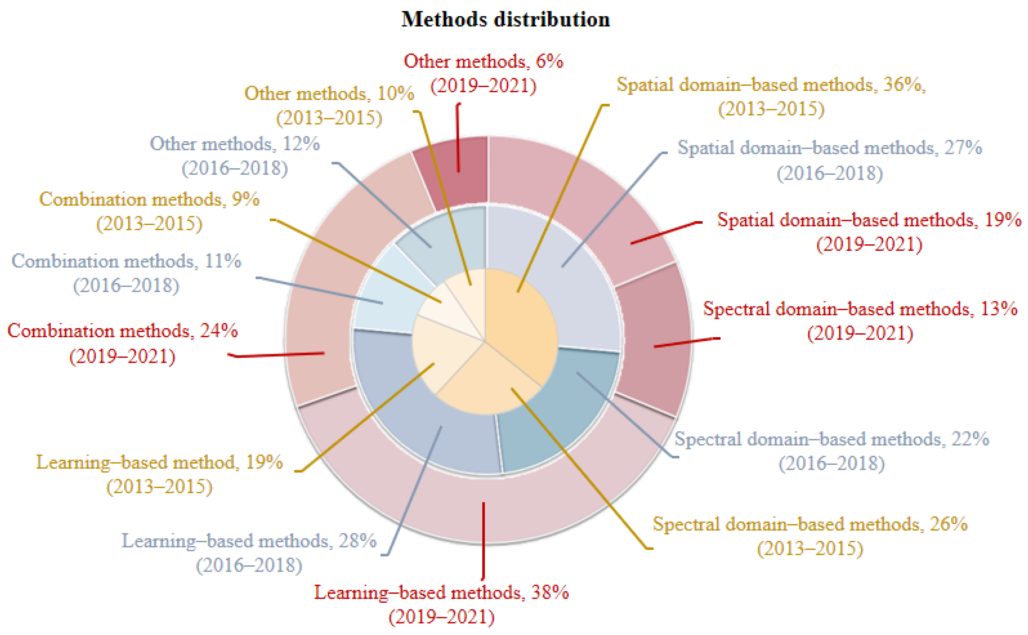
3. Bibliometrics Analysis

3.1. Research Distribution Trend Analysis

This paper evaluates the research distribution across the time period (2013 to 2015, 2016 to 2018 and 2019 to 2021) on no-reference image quality evaluation in recent years. In the above three periods, 74, 92 and 105 related papers were published, respectively. The distribution of methods used in related papers is shown in Figure 8. We also found that from 2013 to 2015, the frequency rankings of search keywords from more to less were spatial domain methods, spectral domain methods and deep learning methods; from 2016 to 2018, the search frequency ranking changed to spatial domain methods, deep learning methods, spectral domain methods and other methods; from 2019 to 2021, the ranking was updated to deep learning methods, combination methods, spatial domain methods, spectral domain methods and other methods.

By analyzing Figure 8, during 2013–2015, the spatial domain-based methods were the most with a percentage of 36, followed by the spectral domain-based methods, while the learning-based methods are only 19% of the total articles. In the following years, the learning-based methods grew rapidly, most possibly owing to the explosion of deep learning techniques. During 2016–2018, the number of methods based on spatial domain and learning was similar, 27% and 28%, respectively. From 2019 to 2021, the majority of the research in image quality evaluation is based on learning, and combination methods also show great potential with a percentage of 24. The learning-based methods are currently the most widely used methods due to their excellent behavior for extracting features automatically. The statistical data related information in our paper comes from Web of Science.

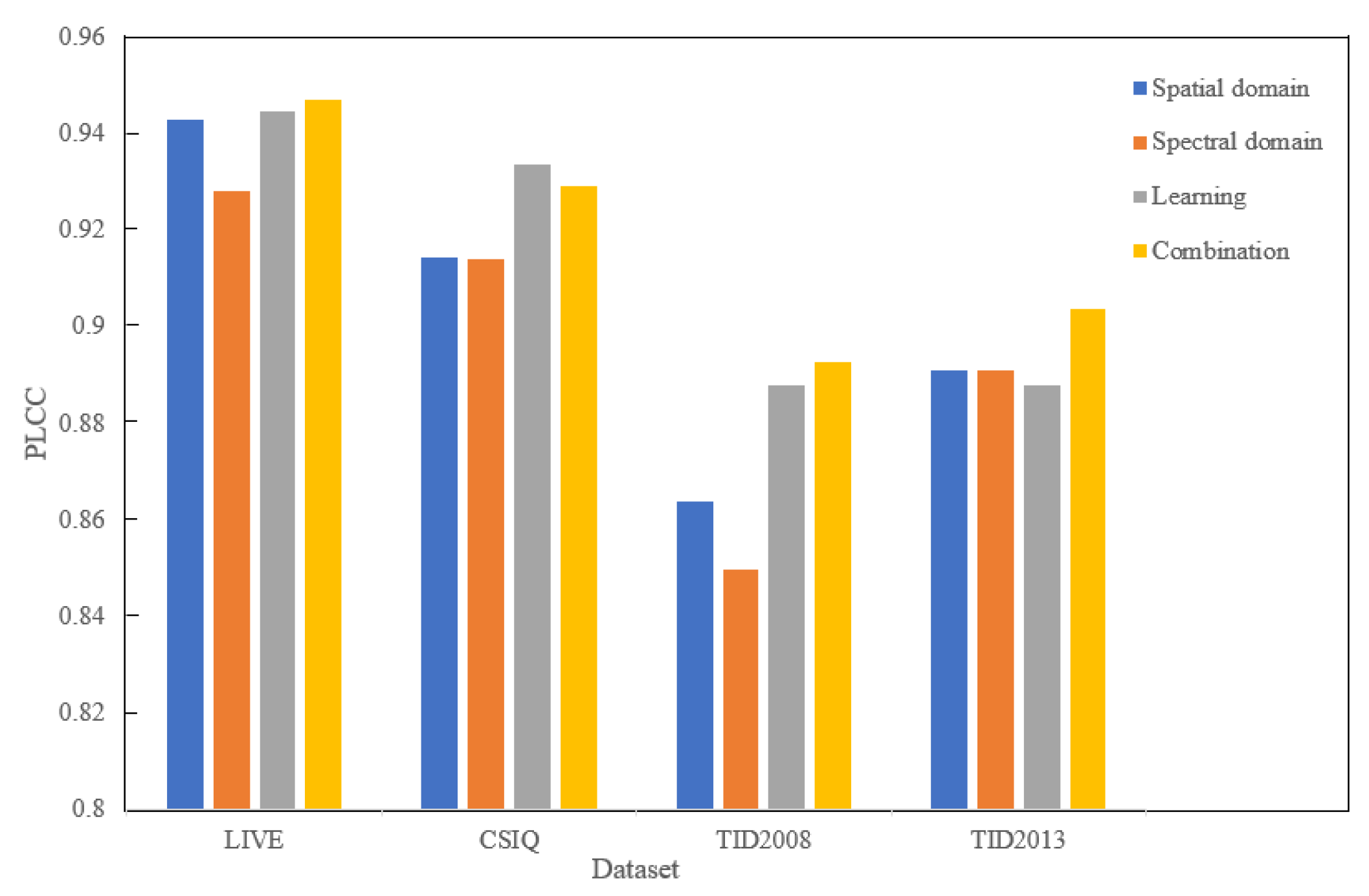
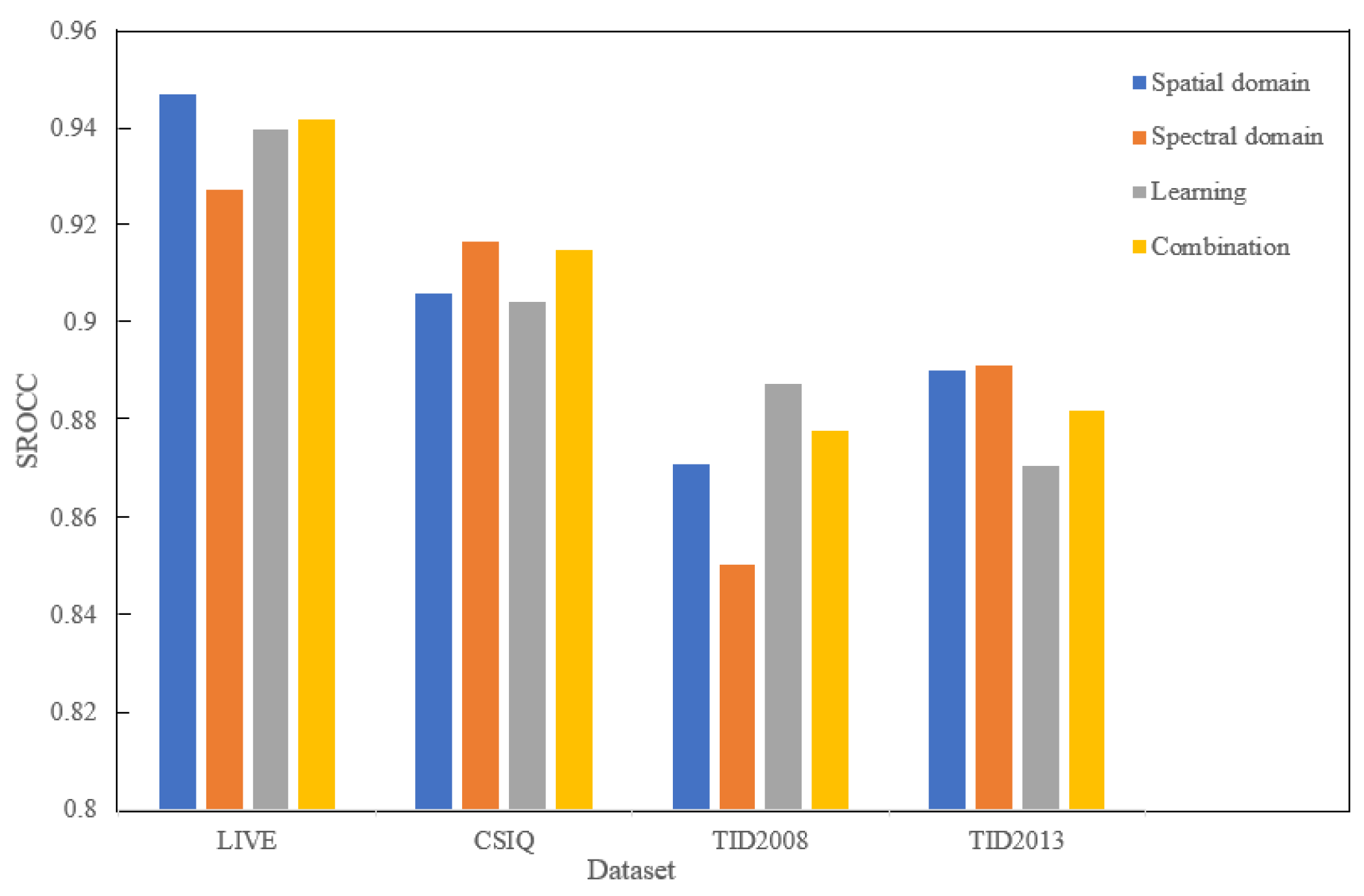
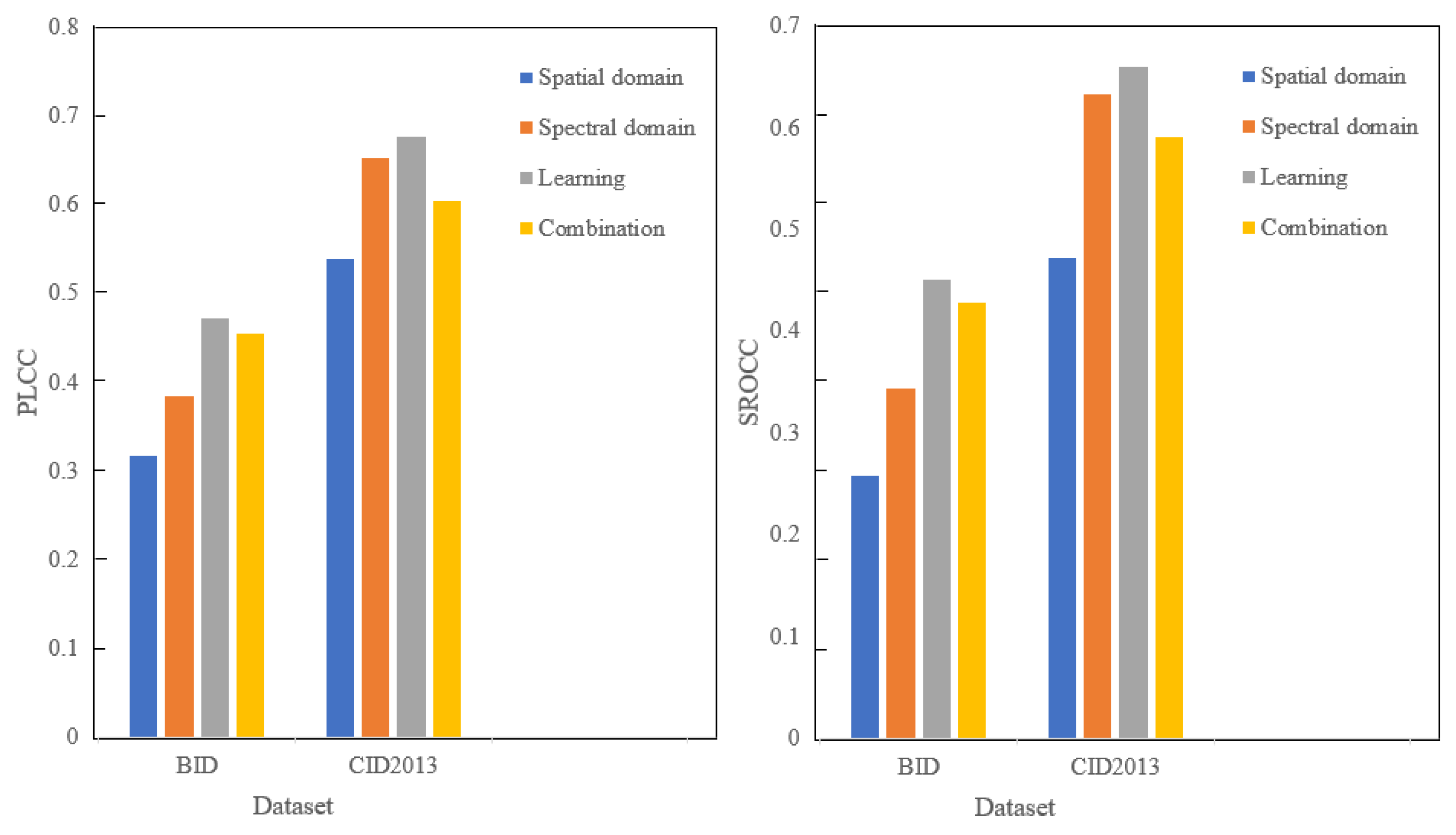
3.2. The Performance of the Representative Methods on Public Datasets

In this section, we selected several representative methods from the above four main groups and analyzed their evaluation performance on the public datasets. MLV [46], BIBLE [35], MGV [46], ARISM [47] and CPBD [49] are selected for the spatial domain-based methods; DCT-QM [60], SC-QI [61], FISH [62], LPC-SI [65] and BISHARP [66] are selected for the spectral domain-based method; BIQI [72], DB-CNN [77], DeepBIQ [78], SPARISH [79], SR [81] and MSFF [87] are selected to represent the learning-based methods; S3 [88], RFSV [91], SVC [92] and SFA [93] are selected as the combination methods. The specific information of the comparison method is described in

Table 3. Specific information of different methods for comparison.

Group	Method Category	Method	Published Time	Characteristic
Spatial domain-based	Grayscale gradient-based	MLV [46]	2014	Calculate the maximum local change in the image
	Grayscale gradient-based	BIBLE [35]	2015	Calculate gradients and Tchebichef moments of images
	Edge detection-based	MGV [46]	2018	Calculate the maximum gradient and gradient change in the image
	Other spatial domain-based	ARISM [47]	2014	Calculate the energy difference and contrast difference of the AR model coefficients for each pixel
	Other spatial domain-based	CPBD [49]	2011	Calculate the cumulative probability of blur detection
Spectral domain-based	Fourier transform-based	DCT-QM [60]	2016	Compute the weighted average L2 norm in the DCT domain.
	Fourier transform-based	SC-QI [61]	2016	Structural contrast indices and DCT blocks are employed to characterize local image features and visual quality perception properties of various distortion types.
	Fourier transform-based	FISH [62]	2022	Compute image derivatives and block-based DFT
	Wavelet transform-based	LPC-SI [65]	2013	Calculate LPC intensity change
	Wavelet transform-based	BISHARP [66]	2018	Calculate the root mean square of the image to obtain local contrast information
Learning-based	Machine-based	BIQI [72]	2010	The NSS model was used to parameterize the sub-band coefficients and to predict the sharpness values.
	Deep learning-based	DB-CNN [77]	2020	Distorted images use two convolutional neural networks for feature extraction and bilinear pooling for quality prediction.
	Deep learning-based	DeepBIQ [78]	2018	Use features extracted from pretrained CNN as generic image descriptions.
	Dictionary learning-based	SPARISH [79]	2016	The image is represented as a block using a dictionary, and the energy of the block is calculated using the sparse coefficient, then normalized by the pooling layer to obtain a sharpness evaluation score.
	Dictionary learning-based	SR [81]	2016	Sparse representation (SR) is used to extract structural information, and a multi-scale spatial max-pooling scheme is introduced to represent image locality.
	Other learning-based	MSFF [87]	2019	Taking multiple features of the image as input and learn feature weights through end-to-end training to obtain evaluations
Combination	Graycale + DCT	S3 [88]	2012	Calculate the slope of the magnitude spectrum in the spectral domain and the spatial variation in the spatial domain of the image patch
	DCT + SIFT	RFSV [91]	2016	The blocks that compute the gradient maps are converted to DCT coefficients to obtain shape information, and scale-invariant feature transform (SIFT) is used to obtain saliency maps.
	SVC + Gradient	SVC [92]	2017	Image quality is characterized using the distribution of different structural changes and the extent of structural differences.
	DCNN + SFA	SFA [93]	2019	The pre-trained DCNN model is used to extract features, and after feature aggregation, the least squares regression is partially used for quality prediction.

. We also introduce six commonly used public datasets and four commonly used indicators in different literature to measure the sharpness methods and to select two indicators to evaluate the image quality evaluation results.

3.2.1. Public Datasets and Evaluation Indicators

The most commonly used datasets in the field include Laboratory for Image and Video Engineer (LIVE) [95], Categorical Subjective Image Quality (CSIQ) [96], Tampere Image Database 2008 (TID2008) [97], Tampere Image Database 2013 (TID2013) [98], Blurred Image Dataset (BID) [99], image dataset from the University of Helsinki CID2013 [100], etc. Among them, LIVE, CSIQ, TID2008 and TID2013 datasets are analog distortion datasets; BID and CID2013 datasets are natural distortion datasets. The specific information of these public datasets is shown in

Table 4. Specific information of the public datasets.

Dataset	Distortion Type	Number of Reference Images	Number of Distorted Images	Image Size (Pixel)	Subjective Scoring	Score Range
LIVE	Analog distortion	29	779	428 × 634–512 × 768	DMOS	[1, 100]
CSIQ	Analog distortion	30	866	512 × 512	DMOS	[0, 9]
TID2008	Analog distortion	25	1700	512 × 384	MOS	[0, 9]
TID2013	Analog distortion	25	3000	512 × 384	MOS	[0, 9]
BID	Natural distortion	-	585	1280 × 960–2272 × 1704	MOS	[0, 5]
CID2013	Natural distortion	-	480	1600 × 1200	MOS	[0, 100]

.

The sharpness performance evaluation indicators are used to determine whether and to what extent the evaluation result of an image sharpness evaluation algorithm is accurate and consistent with the subjective human judgment, which requires certain standards. The most commonly used sharpness performance evaluation indicators are Pearson Linear Correlation Coefficient (PLCC), Spearman’s rank ordered correlation coefficient (SROCC), Kendall Rank Order Correlation Coefficient (KROCC) and Root Mean Square Error (RMSE).

Pearson Linear Correlation Coefficient (PLCC) describes the correlation between the algorithm evaluation value and the human subjective score. It is mainly used to calculate the accuracy, as shown in Equation (1).

$$\mathrm{PLCC}=\frac{1}{n-1}{\sum }_{i=1}^n\left(\frac{x_i-\overline{x}}{{\sigma }_x}\right)\left(\frac{y_i-\overline{y}}{{\sigma }_y}\right)$$

(1)

where $\overline{x}$ and $\overline{y}$ are the mean values of x_i and y_i, respectively, and ${\sigma }_i$ is the corresponding standard deviation.

Spearman’s rank ordered correlation coefficient (SROCC) is mainly used to measure the monotonicity of algorithm prediction, as shown in Equation (2).

$$\mathrm{SROCC}=1-\frac{1}{n\left(n^2-1\right)}{\sum }_{i=1}^n{(r_{xi}-r_{yi})}^2$$

(2)

where r_xi and r_yi are the sorting positions of xi and yi in their respective data sequences.

Kendall Rank Order Correlation Coefficient (KROCC) can also effectively measure the monotonicity of the algorithm, as shown in Equation (3).

$$\mathrm{KROCC}=\frac{2n_c-n_d}{n\left(n-1\right)}$$

(3)

where n_c is the number of consistent element pairs in the dataset and n_d is the number of inconsistent element pairs in the dataset.

Root Mean Square Error (RMSE) is used to directly measure the absolute error between the algorithm evaluation score and the human subjective score, as shown in Equation (4).

$$\mathrm{RMSE}={\left[\frac{1}{n}{\sum }_{i-1}^n{\left(x_i-y_i\right)}^2\right]}^{\frac{1}{2}}$$

(4)

where x_i is the subjective MOS value and y_i is the predicted score of the algorithm.

3.2.2. Performance Analysis of Representative Methods

To observe the performance of various no-reference image quality evaluation methods, this paper compares several representative methods on several public datasets. PLCC and SROCC are adopted to assess the image quality evaluation results. The experimental results in the table are taken from the reported references, and each comparison method group was tested on the same dataset. The comparison of different evaluation methods on the LIVE dataset and CSIQ dataset, TID2008 dataset and TID2013 dataset, BID dataset and CID2013 dataset are shown in

Table 5. Comparison of different evaluation methods on LIVE dataset and CSIQ dataset.

Group	Method	LIVE		CSIQ
		PLCC	SROCC	PLCC	SROCC
Spatial domain-based	MLV [46]	0.938	0.937	0.894	0.851
	BIBLE [35]	0.962	0.961	0.940	0.913
	MGV [46]	0.960	0.963	0.907	0.950
	ARISM [47]	0.959	0.956	0.948	0.931
	CPBD [49]	0.895	0.918	0.882	0.885
Spectral domain-based	DCT-QM [60]	0.925	0.938	0.872	0.926
	SC-QI [61]	0.937	0.948	0.927	0.943
	FISH [62]	0.904	0.841	0.923	0.894
	LPC-SI [65]	0.922	0.950	0.906	0.893
	BISHARP [66]	0.952	0.960	0.942	0.927
Learning-based	BIQI [72]	0.920	0.914	0.846	0.773
	DB-CNN [77]	0.970	0.968	0.959	0.946
	DeepBIQ [78]	0.912	0.893	0.975	0.967
	SPARISH [79]	0.956	0.959	0.938	0.914
	SR [81]	0.961	0.955	0.950	0.921
	MSFF [87]	0.949	0.950	-	-
Combination	S3 [88]	0.943	0.944	0.893	0.911
	RFSV [91]	0.974	0.971	0.942	0.920
	SVC [92]	0.949	0.941	0.952	0.954
	SFA [93]	0.942	0..953	-	-

,

Table 6. Comparison of different evaluation methods on TID2008 dataset and TID2013 dataset.

Group	Method	TID2008		TID2013
		PLCC	SROCC	PLCC	SROCC
Spatial domain-based	MLV [46]	0.811	0.812	0.883	0.879
	BIBLE [35]	0.893	0.892	0.905	0.898
	MGV [46]	0.937	0.942	0.914	0.921
	ARISM [47]	0.854	0.868	0.898	0.902
	CPBD [49]	0.824	0.841	0.855	0.852
Spectral domain-based	DCT-QM [60]	0.819	0.837	0.852	0.854
	SC-QI [61]	0.890	0.905	0.907	0.905
	FISH [62]	0.816	0.786	0.911	0.912
	LPC-SI [65]	0.846	0.843	0.892	0.889
	BISHARP [66]	0.877	0.880	0.892	0.896
Learning-based	BIQI [72]	0.794	0.799	0.825	0.815
	DB-CNN [77]	0.873	0.859	0.865	0.816
	DeepBIQ [78]	0.951	0.952	0.920	0.922
	SPARISH [79]	0.889	0.887	0.900	0.893
	SR [81]	0.895	0.911	0.899	0.892
	MSFF [87]	0.926	0.917	0.917	0.922
Combination	S3 [88]	0.851	0.842	0.879	0.861
	RFSV [91]	0.915	0.924	0.924	0.932
	SVC [92]	0.889	0.874	0.857	0.787
	SFA [93]	0.916	0.907	0.954	0.948

and

Table 7. Comparison of different evaluation methods on BID dataset and CID2013 dataset.

Group	Method	BID		CID2013
		PLCC	SROCC	PLCC	SROCC
Spatial domain-based	MLV [46]	0.375	0.317	0.689	0.621
	BIBLE [35]	0.392	0.361	-	-
	MGV [46]	0.307	0.201	0.511	0.499
	ARISM [47]	0.193	0.151	-	-
	CPBD [49]	-	-	0.418	0.293
Spectral domain-based	DCT-QM [60]	0.383	0.376	0.662	0.653
	SC-QI [61]	-	-	-	-
	FISH [62]	0.485	0.474	0.638	0.587
	LPC-SI [65]	0.315	0.216	0.634	0.609
	BISHARP [66]	0.356	0.307	0.678	0.681
Learning-based	BIQI [72]	0.513	0.472	0.742	0.723
	DB-CNN [77]	0.471	0.464	0.686	0.672
	DeepBIQ [78]	-	-	-	-
	SPARISH [79]	0.482	0.402	0.661	0.652
	SR [81]	0.415	0.467	0.621	0.634
	MSFF [87]	-	-	-	-
Combination	S3 [88]	0.427	0.425	0.687	0.646
	RFSV [91]	0.391	0.335	0.701	0.694
	SVC [92]	-	-	0.425	0.433
	SFA [93]	0.546	0.526	-	-

, respectively.

As can be seen from Table 5, RFSV and DeepBIQ have the highest score and best performance on the LIVE and CSIQ analog distortion databases, respectively. Table 6 shows that DeepBIQ and SFA have the highest PLCC and SROCC values and the best performance on TID2008 and TID2013 analog distortion databases, respectively. From Table 7, the best performers on BID and CID2013 natural distortion datasets are SFA and BIQI, respectively. The spatial domain-based methods are generally based on basic image processing, with the obtained results intuitive. However, although the low-level features extracted with spatial domain-based methods are rich in local details, global semantic information is missing, causing the evaluation accuracy to be unsatisfactory. The performance of the spectral domain-based methods tends to fluctuate significantly depending on different datasets, to be specific, well-performed on analog distortion datasets while less effect on natural distortion datasets. It is because the spectral domain-based methods are excellent on high-frequency detail information analysis. The learning-based methods outperform other methods on the analog distortion datasets, but the performance on the four natural distortion datasets varies greatly. Combination methods can flexibly combine the above methods in a variety of ways to meet the characteristics of different images, thus could achieve good scores on their target dataset. However, currently, no one method can guarantee the optimal effect on all datasets.

Figure 9 and Figure 10 are the PLCC and SROCC values of different groups of methods on the analog distortion datasets, respectively, and Figure 11 shows the PLCC and SROCC values of different groups of methods on the natural distortion datasets. The data in Figure 9, Figure 10 and Figure 11 are all taken from the average of the comparison results in Table 5, Table 6 and Table 7. It can be concluded that most of the methods based on spatial-domain and combination methods perform well in the analog distortion datasets. Meanwhile, the learning-based methods show great potential in the comprehensive performance of both analog and natural distortion datasets.

4. Conclusions and Outlook

Through the evolution of no-reference image sharpness assessment research, from traditional methods (spatial or spectral domain-based) to learning-based methods to methods combination, this technique has witnessed rapid development in itself. The following conclusions can be raised by analyzing a large number of works of literature.

(1) Each group of evaluation methods is inseparable from the feature extraction process. The spatial domain-based feature extraction is simple and efficient, which is beneficial for real-time applications, but easily interfered by image noise. The spectral domain feature extraction can effectively remove noise but at the cost of increased time complexity. Reported research reveals that the reasonable selection of the combination in spatial and spectral domains helps improve the accuracy in image quality evaluation [101,102]. In the learning-based method, the machine learning-based method mainly extracts features manually. With the wide application of deep learning methods, CNN-based feature extraction has become a popular trend for scholars.

(2) In recent years, methods based on deep learning have achieved good results in evaluating no-reference image clarity. However, due to the complexity of the deep learning network model, a large amount of training data is often required. Actually, it is quite difficult to collect enough real-world images for network training, making it urgent to design a deep learning evaluation method suitable for small-scale datasets.

In the future research, the sharpness evaluation method combining multiple methods will gradually become a popular trend. We believe that the overall evaluation performance can be further improved by using the deep learning network model to extract features, combined with the high real-time performance in the image space domain and interference elimination in the spectral domain. To summarize, image quality evaluation research has the potential for further development of new research ideas on the ways in practical application in real-world image datasets and taking full advantage of combined methods.

References

1. Mahajan, P.; Jakhetiya, V.; Abrol, P.; Lehana, P.K.; Guntuku, S.C. Perceptual quality evaluation of hazy natural images. IEEE Trans. Ind. Inform. 2021, 17, 8046–8056. [Google Scholar] [CrossRef]
2. Li, Y.L.; Jiang, Y.J.; Yu, X.; Ren, B.; Wang, C.Y.; Chen, S.H.; Su, D.Y. Deep-learning image reconstruction for image quality evaluation and accurate bone mineral density measurement on quantitative CT: A phantom-patient study. Front. Endocrinol. 2022, 13, 884306. [Google Scholar] [CrossRef] [PubMed]
3. Zhang, Y.Q.; Chen, H.; Wang, L.; Xiao, Y.J.; Huang, H.B. Color image segmentation using level set method with initialization mask in multiple color spaces. Int. J. Eng. Manuf. 2011, 1, 70–76. [Google Scholar] [CrossRef] [Green Version]
4. Dickmann, J.; Sarosiek, C.; Rykalin, V.; Pankuch, M.; Coutrakon, G.; Johnson, R.P.; Bashkirov, V.; Schulte, R.W.; Parodi, K.; Landry, G.; et al. Proof of concept image artifact reduction by energy-modulated proton computed tomography (EMpCT). Phys. Med. 2021, 81, 237–244. [Google Scholar] [CrossRef] [PubMed]
5. Liu, S.Q.; Yu, S.; Zhao, Y.M.; Tao, Z.; Yu, H.; Jin, L.B. Salient region guided blind image sharpness assessment. Sensors 2021, 21, 3963. [Google Scholar] [CrossRef]
6. David, K.; Mehmet, C.; Xiaoping, A.S. State estimation based echolocation bionics and image processing based target pattern recognition. Adv. Sci. Technol. Eng. Syst. 2019, 4, 73–83. [Google Scholar]
7. Ke, Z.X.; Yu, L.J.; Wang, G.; Sun, R.; Zhu, M.; Dong, H.R.; Xu, Y.; Ren, M.; Fu, S.D.; Zhi, C. Three-Dimensional modeling of spun-bonded nonwoven meso-structures. Polymers 2023, 15, 600. [Google Scholar] [CrossRef]
8. Zhu, H.; Zhi, C.; Meng, J.; Wang, Y.; Liu, Y.; Wei, L.; Fu, S.; Miao, M.; Yu, L. A self-pumping dressing with multiple liquid transport channels for wound microclimate management. Macromol. Biosci. 2022, 23, 2200356. [Google Scholar] [CrossRef]
9. Wang, Z.; Bovik, A.C. Reduced- and no-reference image quality assessment. IEEE Signal Process. Mag. 2011, 28, 29–40. [Google Scholar] [CrossRef]
10. Wu, Q.; Li, H.; Meng, F.; Ngan, K.N.; Zhu, S.Y. No reference image quality assessment metric via multi-domain structural information and piecewise regression. Vis. Commun. Image Represent. 2015, 32, 205–216. [Google Scholar] [CrossRef]
11. Lu, Y.; Xie, F.; Liu, T.; Jiang, Z.J.; Tao, D.C. No reference quality assessment for multiply-distorted images based on an improved bag-of-words model. IEEE Signal Process. Lett. 2015, 22, 1811–1815. [Google Scholar] [CrossRef]
12. Cai, H.; Wang, M.J.; Mao, W.D.; Gong, M.L. No-reference image sharpness assessment based on discrepancy measures of structural degradation. J. Vis. Commun.. Image Represent. 2020, 71, 102861. [Google Scholar] [CrossRef]
13. Qi, L.Z.; Zhi, C.; Meng, J.G.; Wang, Y.Z.; Liu, Y.M.; Song, Q.W.; Wu, Q.; Wei, L.; Dai, Y.; Zou, J.; et al. Highly efficient acoustic absorber designed by backing cavity-like and filled-microperforated plate-like structure. Mater. Des. 2023, 225, 111484. [Google Scholar] [CrossRef]
14. Chen, G.; Zhai, M. Quality assessment on remote sensing image based on neural networks. J. Vis. Commun. Image Represent. 2019, 63, 102580. [Google Scholar] [CrossRef]
15. Huang, S.; Liu, Y.; Du, H. A no-reference objective image sharpness metric for perception and estimation. Sixth Int. Conf. Digit. Image Process. (ICDIP 2014) 2014, 915914, 1–7. [Google Scholar]
16. Ferzli, R.; Karam, L.J. A no-reference objective image sharpness metric based on the notion of just noticeable blur (JNB). IEEE Trans. Image Process. A Publ. IEEE Signal Process. Soc. 2009, 18, 717–728. [Google Scholar] [CrossRef]
17. Qian, J.Y.; Zhao, H.J.; Fu, J.; Song, W.; Qian, J.D.; Xiao, Q.B. No-reference image sharpness assessment via difference quotients. Electron. Imaging 2019, 28, 013032. [Google Scholar] [CrossRef]
18. Zhai, G.T.; Min, X.K. Perceptual image quality assessment: A survey. Sci. China Inf. Sci. 2020, 63, 211301. [Google Scholar] [CrossRef]
19. Mittal, A.; Moorthy, A.K.; Bovik, A.C. No-reference image quality assessment in the spatial domain. IEEE Trans. Image Process. 2012, 21, 4695–4708. [Google Scholar] [CrossRef]
20. Li, Q.; Lin, W.; Fang, Y. No-reference quality assessment for multiply-distorted images in gradient domain. IEEE Signal Process. Lett. 2016, 23, 541–545. [Google Scholar] [CrossRef]
21. Bovik, A.C.; Liu, S. DCT-domain blind measurement of blocking artifacts in DCT-coded images. In Proceedings of the IEEE International Conference on Acoustics, Speech, and Signal Processing, Salt Lake City, UT, USA, 7–11 May 2001; Volume 3, pp. 1725–1728. [Google Scholar]
22. Hou, W.L.; Gao, X.B.; Tao, D.C.; Li, X.L. Blind image quality assessment via deep learning. IEEE Trans. Neural Netw. Learn. Syst. 2015, 26, 1275–1286. [Google Scholar] [PubMed]
23. Zhang, Y.; Ngan, K.N.; Ma, L.; Li, H.L. Objective quality assessment of image retargeting by incorporating fidelity measures and inconsistency detection. IEEE Trans. Image Process. 2017, 26, 5980–5993. [Google Scholar] [CrossRef] [PubMed]
24. Thakur, N. An efficient image quality criterion in spatial domain. Indian J. Sci. Technol. 2016, 9, 1–6. [Google Scholar]
25. Hong, Y.Z.; Ren, G.Q.; Liu, E.H. A no-reference image blurriness metric in the spatial domain. Opt.-Int. J. Light Electron. Opt. 2016, 127, 5568–5575. [Google Scholar] [CrossRef]
26. Feichtenhofer, C.; Fassold, H.; Schallauer, P. A perceptual image sharpness metric based on local edge gradient analysis. IEEE Signal Process. Lett. 2013, 20, 379–382. [Google Scholar] [CrossRef]
27. Yan, X.Y.; Lei, J.; Zhao, Z. Multidirectional gradient neighbourhood-weighted image sharpness evaluation algorithm. Math. Probl. Eng. 2020, 1, 7864024. [Google Scholar] [CrossRef] [Green Version]
28. Min, X.; Zhai, G.; Gu, K.; Yang, X.; Guan, X. Objective quality evaluation of dehazed images. IEEE Trans. Intell. Transp. Syst. 2019, 20, 2879–2892. [Google Scholar] [CrossRef]
29. Wang, F.; Chen, J.; Zhong, H.N.; Ai, Y.B.; Zhang, W.D. No-Reference image quality assessment based on image multi-scale contour prediction. Appl. Sci. 2022, 12, 2833. [Google Scholar] [CrossRef]
30. Wang, T.G.; Zhu, L.; Cao, P.L.; Liu, W.J. Research on Vickers hardness image definition evaluation function. Adv. Mater. Res. 2010, 121, 134–138. [Google Scholar] [CrossRef]
31. Dong, W.; Sun, H.W.; Zhou, R.X.; Chen, H.M. Autofocus method for SAR image with multi-blocks. J. Eng. 2019, 19, 5519–5523. [Google Scholar] [CrossRef]
32. Jiang, S.X.; Zhou, R.G.; Hu, W.W. Quantum image sharpness estimation based on the Laplacian operator. Int. J. Quantum Inf. 2020, 18, 2050008. [Google Scholar] [CrossRef]
33. Zeitlin, A.D.; Strain, R.C. Augmenting ADS-B with traffic information service-broadcast. IEEE Aerosp. Electron. Syst. Mag. 2003, 18, 13–18. [Google Scholar] [CrossRef]
34. Zhan, Y.B.; Zhang, R. No-Reference image sharpness assessment based on maximum gradient and variability of gradients. IEEE Trans. Multimed. 2017, 20, 1796–1808. [Google Scholar] [CrossRef]
35. Li, L.D.; Lin, W.S.; Wang, X.S.; Yang, G.B.; Bahrami, K.; Kot, A.C. No-reference image blur assessment based on discrete orthogonal moments. IEEE Trans. Cybern. 2015, 46, 39–50. [Google Scholar] [CrossRef]
36. Zhang, K.N.; Huang, D.; Zhang, B.; Zhang, D. Improving texture analysis performance in biometrics by adjusting image sharpness. Pattern Recognit. 2017, 66, 16–25. [Google Scholar] [CrossRef]
37. Sun, R.; Lei, T.; Chen, Q.; Wang, Z.X.; Du, X.G.; Zhao, W.Q. Survey of image edge detection. Front. Signal Process. 2022, 2, 1–13. [Google Scholar] [CrossRef]
38. Dong, L.; Zhou, J.; Tang, Y.Y. Effective and fast estimation for image sensor noise via constrained weighted least squares. IEEE Trans. Image Process. 2018, 27, 2715–2730. [Google Scholar] [CrossRef]
39. Xu, Z.Q.; Ji, X.Q.; Wang, M.J.; Sun, X.B. Edge detection algorithm of medical image based on Canny operator. J. Phys. Conf. Ser. 2021, 1955, 012080. [Google Scholar] [CrossRef]
40. Ren, X.; Lai, S.N. Medical image enhancement based on Laplace transform, Sobel operator and Histogram equalization. Acad. J. Comput. Inf. Sci. 2022, 5, 48–54. [Google Scholar]
41. Balochian, S.; Baloochian, H. Edge detection on noisy images using Prewitt operator and fractional order differentiation. Multimed. Tools Appl. 2022, 81, 9759–9770. [Google Scholar] [CrossRef]
42. Marziliano, P.; Dufaux, F.; Winkler, S.; Ebrahimi, T. Perceptual blur and ringing metrics: Application to JPEG2000. Signal Process. Image Commun. 2004, 19, 163–172. [Google Scholar] [CrossRef] [Green Version]
43. Zhang, R.K.; Xiao, Q.Y.; Du, Y.; Zuo, X.Y. DSPI filtering evaluation method based on Sobel operator and image entropy. IEEE Photonics J. 2021, 13, 7800110. [Google Scholar] [CrossRef]
44. Liu, Z.Y.; Hong, H.J.; Gan, Z.H.; Wang, J.H.; Chen, Y.P. An improved method for evaluating image sharpness based on edge information. Appl. Sci. 2022, 12, 6712. [Google Scholar] [CrossRef]
45. Chen, M.Q.; Yu, L.J.; Zhi, C.; Sun, R.J.; Zhu, S.W.; Gao, Z.Y.; Ke, Z.X.; Zhu, M.Q.; Zhang, Y.M. Improved faster R-CNN for fabric defect detection based on Gabor filter with genetic algorithm optimization. Comput. Ind. 2022, 134, 103551. [Google Scholar] [CrossRef]
46. Bahrami, K.; Kot, A.C. A fast approach for no-reference image sharpness assessment based on maximum local variation. IEEE Signal Process. Lett. 2014, 21, 751–755. [Google Scholar] [CrossRef]
47. Gu, K.; Zhai, G.T.; Lin, W.S.; Yang, X.K.; Zhang, W.J. No-reference image sharpness assessment in autoregressive parameter space. IEEE Trans. Image Process. 2015, 24, 3218–3231. [Google Scholar]
48. Chang, H.W.; Zhang, Q.W.; Wu, Q.G.; Gan, Y. Perceptual image quality assessment by independent feature detector. Neurocomputing 2015, 151, 1142–1152. [Google Scholar] [CrossRef]
49. Narvekar, N.D.; Karam, L.J. A no-reference image blur metric based on the cumulative probability of blur detection (CPBD). IEEE Trans. Image Process. 2011, 20, 2678–2683. [Google Scholar] [CrossRef]
50. Lin, L.H.; Chen, T.J. A novel scheme for image sharpness using inflection points. Int. J. Imaging Syst. Technol. 2020, 30, 1–8. [Google Scholar] [CrossRef]
51. Zhang, F.Y.; Roysam, B. Blind quality metric for multidistortion images based on cartoon and texture decomposition. IEEE Signal Process. Lett. 2016, 23, 1265–1269. [Google Scholar] [CrossRef]
52. Anju, M.; Mohan, J. Deep image compression with lifting scheme: Wavelet transform domain based on high-frequency subband prediction. Int. J. Intell. Syst. 2021, 37, 2163–2187. [Google Scholar] [CrossRef]
53. Marichal, X.; Ma, W.Y.; Zhang, H. Blur determination in the compressed domain using DCT information. In Proceedings of the IEEE International Conference on Image Processing, Kobe, Japan, 24–28 October 1999; pp. 386–390. [Google Scholar]
54. Mankar, R.; Gajjela, C.C.; Shahraki, F.F.; Prasad, S.; Mayerich, D.; Reddy, R. Multi-modal image sharpening in fourier transform infrared (FTIR) microscopy. The Analyst 2021, 146, 4822. [Google Scholar] [CrossRef] [PubMed]
55. Wang, H.; Li, C.F.; Guan, T.X.; Zhao, S.H. No-reference stereoscopic image quality assessment using quaternion wavelet transform and heterogeneous ensemble learning. Displays 2021, 69, 102058. [Google Scholar] [CrossRef]
56. Pan, D.; Shi, P.; Hou, M.; Ying, Z.; Fu, S.; Zhang, Y. Blind predicting similar quality map for image quality assessment. In Proceedings of the IEEE Conference on Computer Vision and Pattern Recognition, Salt Lake City, UT, USA, 18–23 June 2018; pp. 6373–6382. [Google Scholar]
57. Golestaneh, S.A.; Chandler, D.M. No-reference quality assessment of JPEG images via a quality relevance map. IEEE Signal Process. Lett. 2014, 21, 155–158. [Google Scholar] [CrossRef]
58. Kanjar, D.; Masilamani, V. Image sharpness measure for blurred images in frequency domain. Procedia Eng. 2013, 64, 149–158. [Google Scholar]
59. Kanjar, D.; Masilamani, V. No-reference image sharpness measure using discrete cosine transform statistics and multivariate adaptive regression splines for robotic applications. Procedia Comput. Sci. 2018, 133, 268–275. [Google Scholar]
60. Bae, S.H.; Kim, M. DCT-QM: A DCT-based quality degradation metric for image quality optimization problems. IEEE Trans. Image Process. 2016, 25, 4916–4930. [Google Scholar] [CrossRef]
61. Bae, S.H.; Kim, M. A novel image quality assessment with globally and locally consilient visual quality perception. IEEE Trans. Image Process. A Publ. IEEE Signal Process. Soc. 2016, 25, 2392–2406. [Google Scholar] [CrossRef]
62. Baig, M.A.; Moinuddin, A.A.; Khan, E.; Ghanbari, M. DFT-based no-reference quality assessment of blurred images. Multimed. Tools Appl. 2022, 81, 7895–7916. [Google Scholar] [CrossRef]
63. Kerouh, F. A no reference quality metric for measuring image blur in wavelet domain. Int. J. Digit. Form. Wirel. Commun. 2012, 4, 803–812. [Google Scholar]
64. Vu, P.V.; Chandler, D.M. A fast wavelet-based algorithm for global and local image sharpness estimation. IEEE Signal Process. Lett. 2012, 19, 423–426. [Google Scholar] [CrossRef]
65. Hassen, R.; Wang, Z.; Salama, M.A. Image sharpness assessment based on local phase coherence. IEEE Trans. Image Process. 2013, 22, 2798–2810. [Google Scholar] [CrossRef]
66. Gvozden, G.; Grgic, S.; Grgic, M. Blind image sharpness assessment based on local contrast map statistics. J. Vis. Commun. Image Represent. 2018, 50, 145–158. [Google Scholar] [CrossRef]
67. Bosse, S.; Maniry, D.; Muller, K.R.; Samek, W. Deep neural networks for no-reference and full-reference image quality assessment. IEEE Trans. Image Process. 2018, 27, 206–219. [Google Scholar] [CrossRef] [PubMed] [Green Version]
68. Burges, C.; Shaked, T.; Renshaw, E. Learning to rank using gradient descent. In Proceedings of the International Conference on Machine Learning, New York, NY, USA, 7 August 2005; pp. 89–96. [Google Scholar]
69. Ye, P.; Kumar, J.; Kang, L. Unsupervised feature learning framework for no-reference image quality assessment. In Proceedings of the IEEE Conference on Computer Vision and Pattern Recognition, Providence, RI, USA, 16–21 June 2012; pp. 1098–1105. [Google Scholar]
70. Pei, B.; Liu, X.; Feng, Z. A No-Reference image sharpness metric based on large-scale structure. J. Phys. Conf. 2018, 960, 012018. [Google Scholar] [CrossRef]
71. Liu, L.; Gong, J.; Huang, H.; Sang, Q.B. Blind image blur metric based on orientation-aware local patterns. Signal Process.-Image Commun. 2020, 80, 115654. [Google Scholar] [CrossRef]
72. Moorthy, A.K.; Bovik, A.C. A two-step framework for constructing blind image quality indices. IEEE Signal Process. Lett. 2010, 17, 513–516. [Google Scholar] [CrossRef]
73. Kim, J.; Nguyen, A.D.; Lee, S. Deep CNN-based blind image quality predictor. IEEE Trans. Neural Netw. Learn. Syst. 2019, 30, 11–24. [Google Scholar] [CrossRef] [PubMed]
74. Zhu, M.L.; Ge, D.Y. Image quality assessment based on deep learning with FPGA implementation. Signal Process. Image Commun. 2020, 83, 115780. [Google Scholar] [CrossRef]
75. Li, D.Q.; Jiang, T.T.; Jiang, M. Exploiting high-level semantics for no-reference image quality assessment of realistic blur images. In Proceedings of the 25th ACM International Conference on Multimedia, Mountain View, CA, USA, 23–27 October 2017; pp. 378–386. [Google Scholar]
76. Lin, K.Y.; Wang, G.X. Hallucinated-IQA: No-reference image quality assessment via adversarial learning. In Proceedings of the 2018 IEEE/CVF Conference on Computer Vision and Pattern Recognition (CVPR), Salt Lake City, UT, USA, 18–23 June 2018; pp. 732–741. [Google Scholar]
77. Zhang, W.X.; Ma, K.D.; Yan, J.; Deng, D.X.; Wang, Z. Blind image quality assessment using a deep bilinear convolutional neural network. IEEE Trans. Circuits Syst. Video Technol. 2020, 30, 36–47. [Google Scholar] [CrossRef] [Green Version]
78. Bianco, S.; Celona, L.; Napoletano, P.; Schettini, R. On the use of deep learning for blind image quality assessment. Signal Image Video Process. 2018, 12, 355–362. [Google Scholar] [CrossRef] [Green Version]
79. Gao, F.; Yu, J.; Zhu, S.G.; Huang, Q.M.; Tian, Q. Blind image quality prediction by exploiting multi-level deep representations. Pattern Recognit. 2018, 81, 432–442. [Google Scholar] [CrossRef]
80. Li, L.; Wu, D.; Wu, J.; Li, H.L.; Lin, W.S.; Kot, A.C. Image sharpness assessment by sparse representation. IEEE Trans. Multimed. 2016, 18, 1085–1097. [Google Scholar] [CrossRef]
81. Lu, Q.B.; Zhou, W.G.; Li, H.Q. A no-reference image sharpness metric based on structural information using sparse representation. Inf. Sci. 2016, 369, 334–346. [Google Scholar] [CrossRef]
82. Xu, J.T.; Ye, P.; Li, Q.H.; Du, H.Q.; Liu, Y.; Doermann, D. Blind image quality assessment based on high order statistics aggregation. IEEE Trans. Image Process. 2016, 25, 4444–4457. [Google Scholar] [CrossRef] [PubMed]
83. Jiang, Q.P.; Shao, F.; Lin, W.S.; Gu, K.; Jiang, G.Y.; Sun, H.F. Optimizing multistage discriminative dictionaries for blind image quality assessment. IEEE Trans. Multimed. 2018, 20, 2035–2048. [Google Scholar] [CrossRef]
84. Wu, Q.B.; Li, H.L.; Ngan, K.; Ma, K.D. Blind image quality assessment using local consistency aware retriever and uncertainty aware evaluator. IEEE Trans. Circuits Syst. Video Technol. 2018, 28, 2078–2089. [Google Scholar] [CrossRef]
85. Deng, C.W.; Wang, S.G.; Li, Z.; Huang, G.B.; Lin, W.S. Content-insensitive blind image blurriness assessment using Weibull statistics and sparse extreme learning machine. IEEE Trans. Syst. Man Cybern.-Syst. 2019, 49, 516–527. [Google Scholar] [CrossRef]
86. Zhang, Y.B.; Wang, H.Q.; Tan, F.F.; Chen, W.J.; Wu, Z.R. No-reference image sharpness assessment based on rank learning. In Proceedings of the 2019 International Conference on Image Processing (ICIP), Taipei, Taiwan, 22–25 September 2019; pp. 2359–2363. [Google Scholar]
87. He, S.Y.; Liu, Z.Z. Image quality assessment based on adaptive multiple Skyline query. Signal Process.-Image Commun. 2019, 80, 115676. [Google Scholar] [CrossRef]
88. Vu, C.T.; Phan, T.D.; Chandler, D.M. S3: A spectral and spatial measure of local perceived sharpness in natural image. IEEE Trans. Image Process. 2012, 21, 934–945. [Google Scholar] [CrossRef]
89. Liu, X.Y.; Jin, Z.H.; Jiang, H.; Miao, X.R.; Chen, J.; Lin, Z.C. Quality assessment for inspection images of power lines based on spatial and sharpness evaluation. IET Image Process. 2022, 16, 356–364. [Google Scholar] [CrossRef]
90. Yue, G.H.; Hou, C.P.; Gu, K.; Zhou, T.W.; Zhai, G.T. Combining local and global measures for DIBR-Synthesized image quality evaluation. IEEE Trans. Image Process. 2018, 28, 2075–2088. [Google Scholar] [CrossRef]
91. Zhang, S.; Li, P.; Xu, X.H.; Li, L.; Chang, C.C. No-reference image blur assessment based on response function of singular values. Symmetry 2018, 10, 304. [Google Scholar] [CrossRef] [Green Version]
92. Zhan, Y.; Zhang, R.; Wu, Q. A structural variation classification model for image quality assessment. IEEE Trans. Multimed. 2017, 19, 1837–1847. [Google Scholar] [CrossRef]
93. Li, D.Q.; Jiang, T.T.; Lin, W.S.; Jiang, M. Which has better visual quality: The clear blue sky or a blurry animal? IEEE Trans. Onmultimedia 2019, 21, 1221–1234. [Google Scholar] [CrossRef]
94. Li, Y.; Po, L.M.; Xu, X. No-reference image quality assessment with shearlet transform and deep neural networks. Neurocomputing 2015, 154, 94–109. [Google Scholar] [CrossRef]
95. Sheikh, H.R.; Sabir, M.F.; Bovik, A.C. A statistical evaluation of recent full reference image quality assessment algorithms. IEEE Trans. Image Process. 2006, 15, 3440–3451. [Google Scholar] [CrossRef] [PubMed]
96. Larson, E.C.; Chandler, D.M. Most apparent distortion: Full-reference image quality assessment and the role of strategy. J. Electron. Imaging 2010, 19, 011006. [Google Scholar]
97. Ponomarenko, N.; Lukin, V.; Zelensky, A. TID2008-a database for evaluation of full-reference visual quality assessment metrics. Adv. Mod. Radio Electron. 2009, 10, 30–45. [Google Scholar]
98. Ponomarenko, N.; Ieremeiev, O.; Lukin, V. Color image database TID2013: Peculiarities and preliminary results. In Proceedings of the European Workshop on Visual Information Processing (EUVIP), Paris, France, 10–12 June 2013; pp. 106–111. [Google Scholar]
99. Ciancio, A.; Da, S.; Said, A.; Obrador, P. No-reference blur assessment of digital pictures based on multifeature classifiers. IEEE Trans. Image Process. 2011, 20, 64–75. [Google Scholar] [CrossRef]
100. Virtanen, T.; Nuutinen, M.; Vaahteranoksa, M.; Oittinen, P. CID2013: A database for evaluating no-reference image quality assessment algorithms. IEEE Trans. Image Process. 2015, 24, 390–402. [Google Scholar] [CrossRef] [PubMed]
101. Varga, D. No-Reference quality assessment of authentically distorted images based on local and global features. J. Imaging 2022, 8, 173. [Google Scholar] [CrossRef] [PubMed]
102. Li, L.D.; Xia, W.H.; Wang, S.Q. No-Reference and robust image sharpness evaluation based on multiscale spatial and spectral features. IEEE Trans. Multimed. 2017, 19, 1030–1040. [Google Scholar] [CrossRef]
Figure 1. Image sharpness evaluation classification.
Applsci 13 02652 g001
Figure 2. The process of the image sharpness evaluation based on the Prewitt operator.
Applsci 13 02652 g002
Figure 3. Edge detection results: (a) Original image; (b) Canny operator; (c) Sobel operator; (d) Prewitt operator.
Applsci 13 02652 g003
Figure 4. The general framework of spectral domain-based methods.
Applsci 13 02652 g004
Figure 5. The process of wavelet decomposition and reconstruction.
Applsci 13 02652 g005
Figure 6. The general framework of learning-based methods.
Applsci 13 02652 g006
Figure 7. The combined framework of combination methods.
Applsci 13 02652 g007
Figure 8. Distribution of evaluation methods.
Applsci 13 02652 g008
Figure 9. PLCC value of different groups of methods on analog distortion datasets.
Applsci 13 02652 g009
Figure 10. SROCC value of different groups of methods on analog distortion datasets.
Applsci 13 02652 g010
Figure 11. PLCC and SROCC values of different groups of methods on natural distortion datasets.
Applsci 13 02652 g011