Visual Exploration of Cycling Semantics with GPS Trajectory Data

Abstract

Cycling—as a sustainable and convenient exercise and travel mode—has become increasingly popular in modern cities. In recent years, with the proliferation of sport apps and GPS mobile devices in daily life, the accumulated cycling trajectories have opened up valuable opportunities to explore the underlying cycling semantics to enable a better cycling experience. In this paper, based on large-scale GPS trajectories and road network data, we mainly explore cycling semantics from two perspectives. On one hand, from the perspective of the cyclists, trajectories could tell their frequently visited sequences of streets, thus potentially revealing their hidden cycling themes, i.e., cyclist behavior semantics. On the other hand, from the perspective of the road segments, trajectories could show the cyclists’ fine-grained moving features along roads, thus probably uncovering the moving semantics on roads. However, the extraction and understanding of such cycling semantics are nontrivial, since most of the trajectories are raw data and it is also difficult to aggregate the dynamic moving features from trajectories into static road segments. To this end, we establish a new visual analytic system called VizCycSemantics for pervasive computing, in which a topic model (i.e., LDA) is used to extract the topics of cyclist behavior semantics and moving semantics on roads, and a clustering method (i.e., k-means ++) is used to further capture the groups of similar cyclists and road segments within the city; finally, multiple interactive visual interfaces are implemented to facilitate the interpretation for analysts. We conduct extensive case studies in the city of Beijing to demonstrate the effectiveness and practicability of our system and also obtain various insightful findings and pieces of advice.

1. Introduction

The context of modern urbanization and fast-paced life reduces people’s daily exercise. Various diseases, such as obesity and cardiovascular diseases, are also increasing. As a convenient way of exercise and travel, cycling not only improves the health of cyclists but is also a sustainable mode of transportation with environmental and social benefits [1]. In recent years, lots of countries have implemented strategies to improve their cycling service and turn it into a safer and more convenient mode of travel [2,3,4,5].

With the proliferation of sports apps and GPS mobile devices in daily life, various sensing devices have recorded a large number of outdoor-recreation cycling trajectories, including Strava, Keep and so on. Generally, such kinds of big data contain rich spatial and temporal information of the cycling in cities, thus opening up valuable opportunities to explore the underlying cycling semantics to enable a better cycling experience. For example, knowing different types of popular cycling (e.g., recreation, commuting) could help cyclists to find the most desirable and suitable routes, and knowing the roads that are difficult to ride could help city planners to build cycling infrastructures in proper locations. Hence, it is quite meaningful to effectively uncover the implicit cycling semantics from large-scale GPS trajectories.

Trajectories traverse a series of streets, and street names may imply geographic and cultural information to the citizens of a city [6]. Thus, by converting the cycling trajectories into a corresponding set of street names, the obtained corpus is able to semantically reveal the riders’ hidden cycling themes, i.e., the behavior semantics of cyclists. For example, a cyclist often rides along the Seine, indicating that he/she is likely to do recreational cycling. Moreover, it is well-recognized that cycling is naturally restricted to the road network. However, existing studies mainly focused on analyzing the cycling from the perspective of cyclists, ignoring the underlying semantics from road segments [7,8]. In fact, road segments could inherently influence many aspects of cycling, e.g., some roads in poor conditions generally indicate an unfavorable or challenging cycling experience. Fortunately, such influences could also be revealed by GPS trajectories. It is because trajectories contain cyclists’ fine-grained moving characteristics on roads, such as smooth or intense, thus explicitly indicating where they are suitable for smooth cycling and where they are challenging for cycling, i.e., the moving semantics on roads. In a nutshell, in this paper, we aim at utilizing large-scale cycling trajectories and road network data to explore cycling semantics in a city from the perspectives of both cyclists and road segments.

However, it is still nontrivial to effectively extract and perceive the underlying cycling semantics. The challenges are threefold. Firstly, due to the GPS noise and other positioning deviations, the study on the raw GPS trajectories would suffer from the uncertainty problem. Secondly, the road segments are static in nature while the cycling passing through the road segments is spatially and temporally dynamic. Consequently, it is difficult to aggregate the dynamic moving features of the trajectories into static road segments, and it needs to be decoupled properly. Thirdly, cycling semantics in the city cannot be intuitively presented through statistical information, which is hard to be perceived especially for users with low or no technical backgrounds, e.g., urban planners [9].

To overcome the above challenges, this paper presents a new visual analytic system for the exploration of cycling semantics. Specifically, to overcome the GPS uncertainty problem, we map the GPS trajectory coordinates from geometrical positions to the set of street names, then construct a high-level and meaningful textual corpus. Similarly, to address the conflict between static roads and dynamic moving features, we also convert the moving attributes on roads (i.e., velocity, acceleration and turning angle) into three kinds of static textual corpora from cycling trajectories. On top of the different corpora, latent Dirichlet allocation (LDA) is used to automatically extract various topics of cycling semantics based on the word probability, thus further reducing the effect of the uncertainty problem or missing GPS records to a certain extent. Moreover, due to the nature and intuitive connection between human beings and computers through interactive visual interfaces, visual analytics is frequently utilized to explore hidden facts/patterns behind raw data [10,11]. Thus, we further implement multiple interactive user interfaces for analysts to facilitate the understanding of cycling semantics in a visualization manner.

The main contributions of this paper can be summarized as follows.

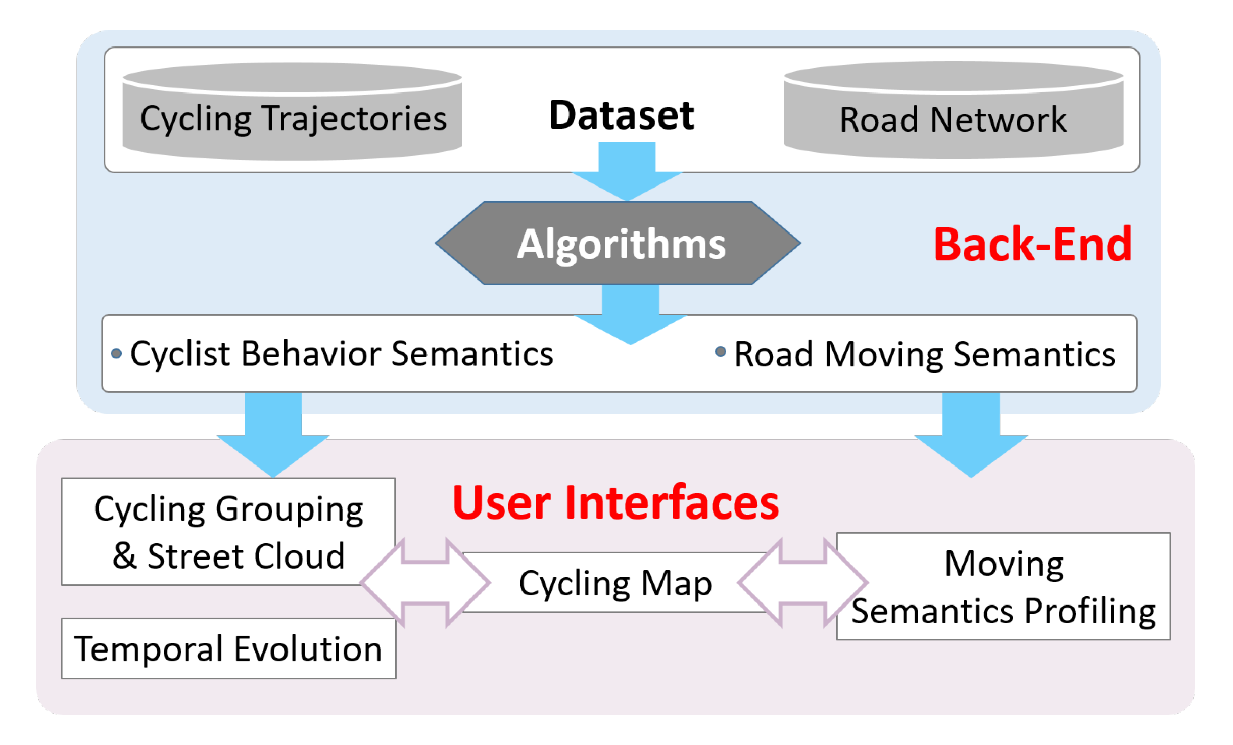
• We propose a new visualization system called VizCycSemantics for the exploration of underlying urban cycling semantics from both the cyclist and road segment’s perspectives, based on large-scale cycling GPS trajectories and road network data. The system could help to improve cycling services in cities.
• We textually convert the cycling trajectories into street name and moving feature corpora, then use a topic model to automatically extract the cyclists’ behavior semantics (i.e., cycling topics of cyclists) and moving semantics on roads (i.e., moving topics on roads), respectively. We further employ a clustering algorithm to capture the groups of similar cyclists and road segments in the city.
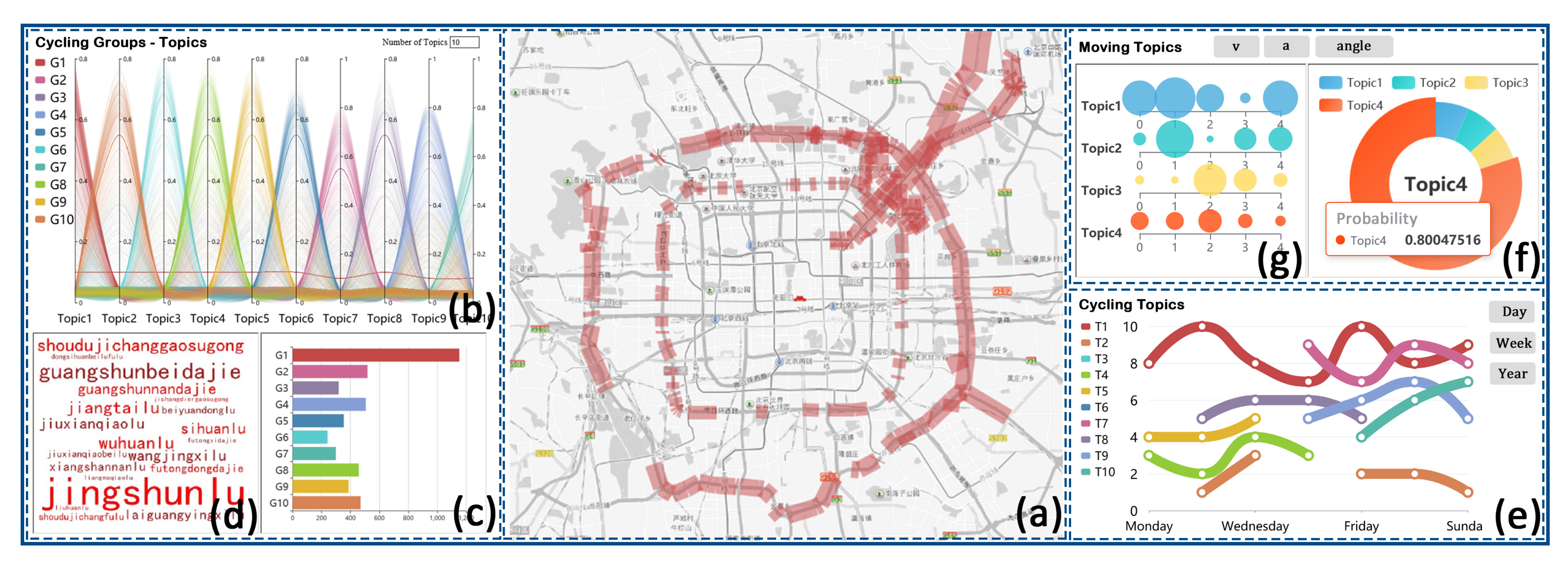
• We implement multiple interfaces to facilitate the understanding of cycling semantics for pervasive computing, including a cycling map, cycling groups and topics, the size of cycling groups, the street cloud of cycling topics, the temporal evolution of cycling topics, moving topics and moving topic distribution. A group of case studies in Beijing demonstrates the effectiveness of our system and also obtains various insightful findings and cycling advice.

The rest of this paper is organized as follows. We review the related work in Section 2. Section 3 describes the system tasks and framework. In Section 4, we elaborate on the details of the backend algorithms. Section 5 provides the data source and visualization designs. We use two cases to demonstrate the effectiveness of our system in Section 6. Finally, Section 7 concludes this paper and discusses future directions.

2. Related Work

In recent years, visualization techniques have become important means for large-scale data exploration [12]. In the transportation community, trajectory data have been widely studied for developing smart urban services [13,14,15,16,17,18,19]; meanwhile, a lot of efforts have also been devoted to the trajectory visualization for a visual mobility analysis [20,21]. Generally, existing visualization works can be broadly categorized into two groups as follows.

2.1. Visualization for Raw and Processed Trajectory Data

The visualization of raw trajectory data is to draw the trajectories without processing, mainly including position animation, time-axis visualization, traffic wall and space–time cube (STC). Furthermore, the space–time cube [22] is a classic method to visualize the multiscale spatiotemporal characteristics of trajectory data. On this basis, Bach et al. [23] proposed a generalized space–time cube which transformed the cube’s 3D shape into readable 2D visualizations. However, the visualization of large-scale raw trajectory data might cause mutual occlusions and visual confusion [12]. To solve the dilemma, visualizations are usually coupled with many processing methods (e.g., trajectory clustering, filtering and compression) to simplify the massive trajectories in time and space. For instance, Chen et al. [10] proposed a visualization method called VAUD, which supported cross-domain correlation and deduction from multiple data sources including taxi trajectory data. Wang et al. [24] presented a visual analysis system to explore sparse traffic trajectory data through applying existing trajectory aggregation techniques to the dataset. Shamal et al. [25] used multiple sketch queries and visualizations to taxi trajectory datasets and discovered historical traffic situations such as speed and volume at specific times, dates and different city locations. The system was built upon a transport database that integrated heterogeneous data sources with an optimized spatial indexing and weighted similarity computation. Krüger et al. [26] presented a visual analytics approach to fine-tune the data preprocessing and matching process, using taxi trajectories to demonstrate the approach in a realistic usage scenario.

2.2. Visualization for Hidden Knowledge of Trajectory Data

Researchers also focus on utilizing visualizations to explore the hidden knowledge and laws implicit in the trajectory data. Brauer et al. [2] quantified urban cycling quality by estimating the fluency of a large set of cycling trajectories, using intuitive visual means. Lu et al. [27] explored the possibility of studying route choice behavior based on a general trajectory dataset. Kamw et al. [28] further proposed a new computation model and visual analytical framework to study the accessibility of urban structures with a taxi trajectory dataset. Moreover, Itoh et al. [29] proposed a visual integration of traffic analysis and social media analysis using smart card data on the Tokyo Metro, Toei Subway. Zeng et al. [30] developed a visual analytics interface that integrated massive human mobility data to explore the relationship between human mobility and activities. Zhao et al. [31] conducted a group-based and individual-based exploration of the passenger’s mobility correlation with a visualization system and examined how passengers differed from or correlated with each other based on the trajectories of buses and subways. Shi et al. [32] surveyed state-of-the-art research works in the visual analytics of anomalous user behaviors with travel data. Feng et al. [33] proposed an accurate and intuitive density for POI accessibility based on the various constraints of road connections and traffic data.

Our work concentrates on visualizing the hidden knowledge of trajectory data. Similar to our work, Chu et al. [6] extracted the taxi topics about the moving behaviors of taxi riders from massive taxi trajectory data within a city, which were displayed and analyzed through a visual analytics system. Additionally, Al-Dohuki et al. [34] managed and visualized taxi trajectory data in a semantic rich means similarly, but they concentrated on the flexibility of semantic query over a text search engine. In this work, we focusd on exploring more diverse and in-depth cycling semantics from two perspectives, namely, the cyclists and the road segments.

3. System Tasks and Framework of VizCycSemantics

In order to enable the systematical exploration of urban cycling semantics, we discussed with collaborative domain experts and carefully summarized three main tasks to motivate the development of our VizCycSemantics system:

• Task 1: Acquire cycling themes of cyclists in the city, i.e., behavior semantics. Based on the cycling trajectories and road network data, find out how many cycling themes of cyclists are in the city, which ones are more popular, how many groups of cyclists there are and how they distribute in time and space. This task could help cyclists to choose the desirable cycling routes and times according to their preferences.
• Task 2: Identify different moving topics of cycling on the road network, i.e., moving semantics on roads. By investigating the fine-grained moving features on road segments, find out the moving topics of road segments in the city and determine where the road network is good for smooth or challenging cycling, where people need to ride with care and so on. This task can enable cyclists to choose appropriate road segments for their physical needs and can also help city planners to properly deploy cycling facilities.
• Task 3: Facilitate the understanding of the cycling semantics for analysts. Through implementing an interactive visualization system, the cycling semantics derived from task 1 and task 2 could be presented more intuitively. The user interfaces should satisfy the criterion of a user-friendly interaction.

Accordingly, our VizCycSemantics system was composed of two modules. As shown in Figure 1, the first one was the backend module, which contained several algorithms to extract cycling semantics automatically from cycling trajectories and road network data. The second module was the user interfaces enabling a visual exploration of cycling semantics according to task 3. We used cycling grouping and a street cloud of cycling topics to show the popular cycling topics and grouping of cyclists and further visualize their temporal evolution of cycling topics. Furthermore, the moving topics and moving topics’ distribution were used to analyze the moving topics of cycling on road segments. Additionally, the cycling map interacted with these interfaces to show the specific spatial distribution of cycling semantics on the map.

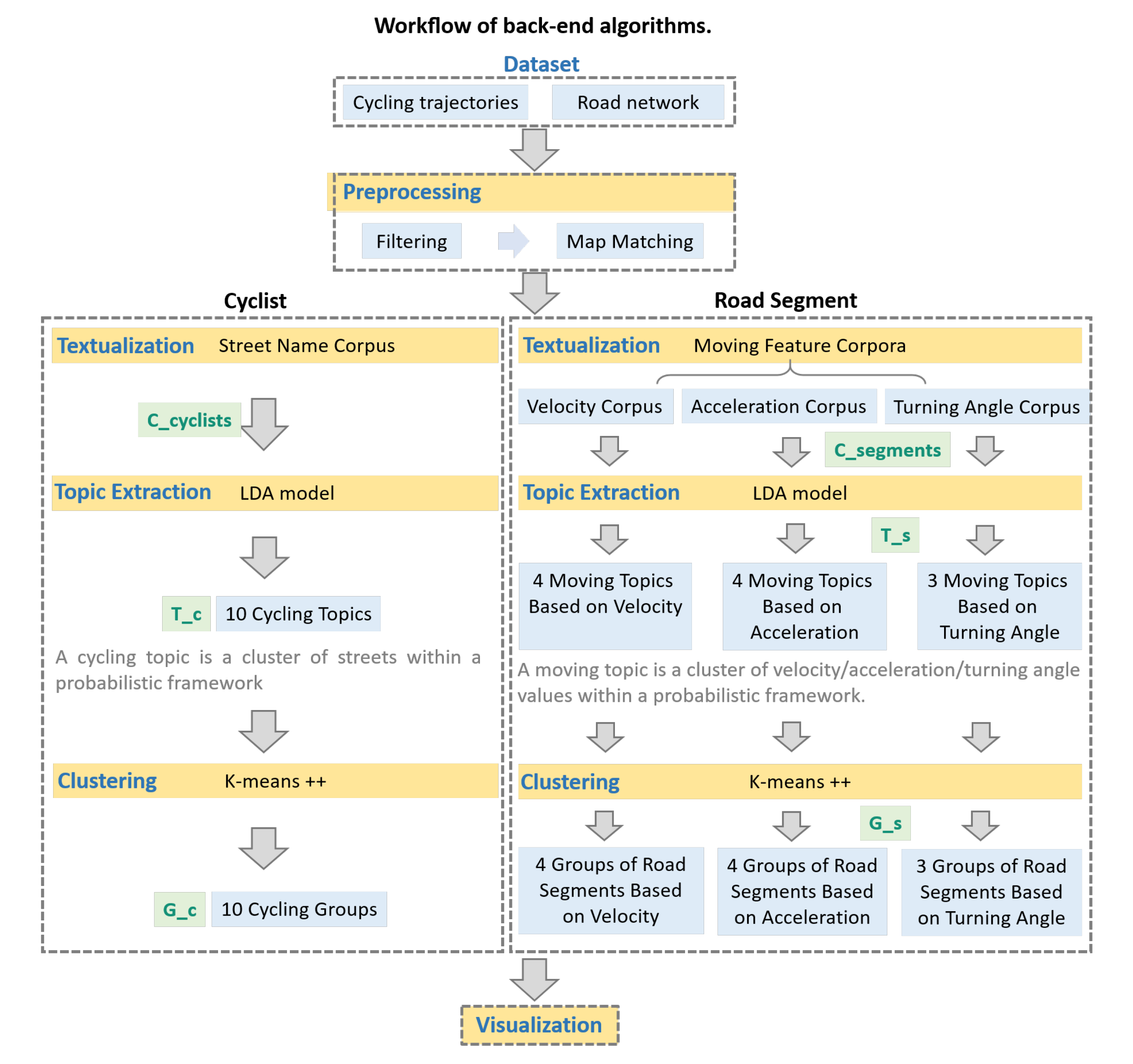
4. Backend Algorithms of VizCycSemantics

Figure 2 illustrates the workflow of the backend algorithms. The inputs were raw cycling trajectories and road network data. In the preprocessing stage, filtering and map matching were used to clean the inputs and derive the matched trajectories to road segments. When the study objects were cyclists, we obtained the street name corpus (i.e., $C\_cyclists$) by converting the trajectories into the corresponding street names. Then, the corpus was sent to the LDA model to capture the cycling topics of cyclists, namely $T\_c$, because the results of the LDA model also provided the probability for each cyclist on all cycling topics. We used k-means ++ [35] to learn the grouping of cyclists, namely $G\_c$. When the study objects were road segments, we extracted three corpora (i.e., $C\_segments$) based on three moving attributes (i.e., velocity, acceleration and turning angle) by converting the trajectories into the corresponding values of moving attributes. Next, in the topic extraction stage, we used the LDA model on each corpus and obtained three aspects of the moving topics (i.e., $T\_s$). Then, in the clustering stage, based on the moving topic distributions extracted from the LDA model, k-means ++ was used to learn the grouping of road segments in the city, namely $G\_s$. Generally, the cycling topics and groups of cyclists (i.e., $T\_c$, $G\_c$) and the moving topics and groups of road segments (i.e., $T\_s$, $G\_s$) were obtained through the backend algorithms and were visualized in user interfaces.

4.1. Preprocessing

We first designated the study area in the city, then filtered out the trajectories that exceeded the area and also deleted duplicated and incomplete ones. On top of that, we utilized the ST-matching algorithm to match the trajectories to the street network [36,37]. ST-matching is based on the hidden Markov model (HMM) [38], which elegantly accounts for measurement noise and the layout of the road network. ST-matching can integrate geometric information and road topology and thus has the advantages of a high precision and good stability. For each trajectory point, the algorithm estimated the emission probability to the nearby street segments and the transition probability. Afterwards, based on the two sets of probabilities, the Viterbi algorithm [39] was used to calculate the optimal sequence of map-matched points.

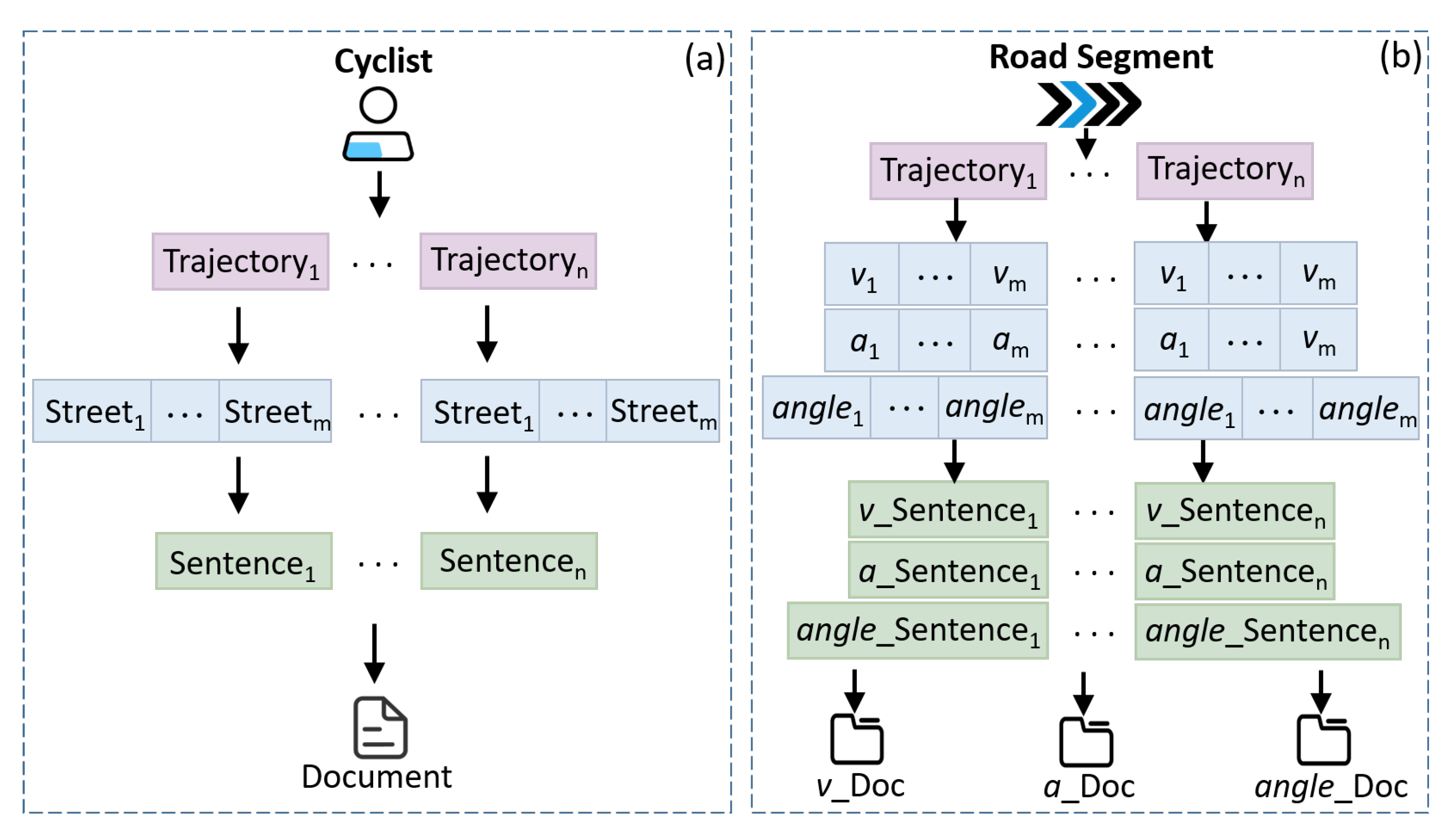
4.2. Textualization

4.2.1. Trajectory–Streets Textualization

Through trajectory textualization, the geometrical positions of cycling trajectories can be transformed to the corresponding street names that could indicate the geographic and cultural information about cyclists [6]. Thus, we could further extract their hidden cycling topics (i.e., behavior semantics of cyclists).

As shown in Figure 3a, a cyclist has n cycling trajectories, and each of them passes through m road segments, while each road segment corresponds to a street name, i.e., a word. Thus, a trajectory can be represented as a sentence with m words. Furthermore, a cyclist can be represented as a document with n sentences. Such a process is carried out for all cyclists. Consequently, we can obtain a corpus regarding the cyclists’ trajectories (i.e., $C\_cyclists$), in which the number of documents equals the number of cyclists.

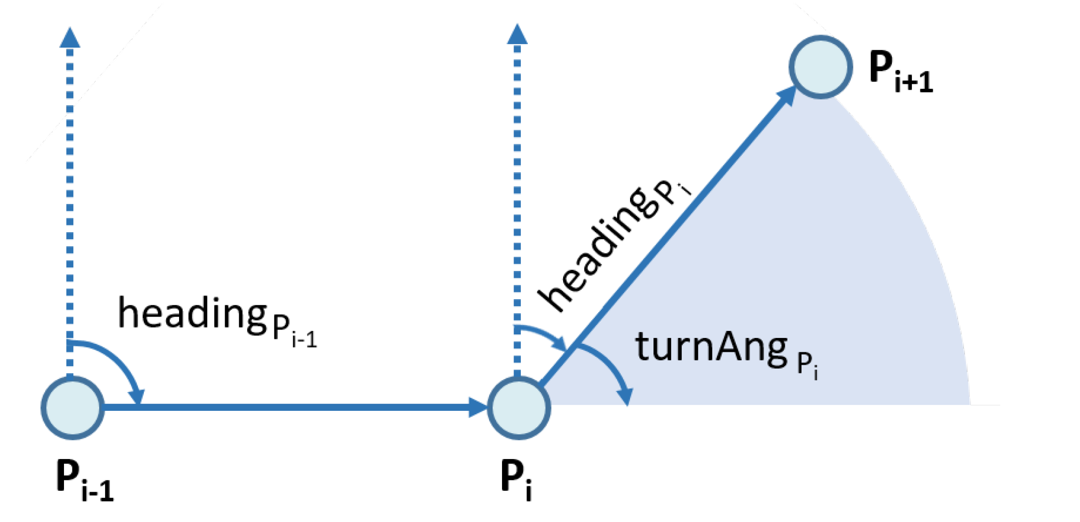
4.2.2. Moving Feature Textualization

As a restriction of cycling, the conditions of the road network strongly influence the cyclist’s movement, thus indicating the moving topics of cycling. In this sense, we textualized the cyclists’ fine-grained moving features on roads from the large-scale GPS trajectories to convey the moving semantics of cycling on the roads.

As shown in Figure 3b, there are n trajectories going through a road segment. For m sampling points in each trajectory, we calculated three moving attributes, including the velocity, acceleration and turning angle. Generally, each moving feature at a point can be viewed as a word, and m words constitute a sentence, e.g., $v_{-}Sentence$. As a result, each trajectory is represented by three sentences with regard to three kinds of moving attributes. Finally, a road segment can be represented as three documents with $3\times n$ sentences, namely, $v_{-}Doc$, $a_{-}Doc$ and $angl{e}_{-}Doc$. By performing the textualization for all road segments, we could obtain three corpora regarding the cycling moving attributes, i.e., $C\_segments$. The details on the computation of the three moving attributes are as follows.

Each trajectory provides a start time $t_s$, end time $t_e$, and a sequence of GPS points with latitudes and longitudes (i.e., $P_1,P_2,P_3,\dots ,P_n$). The Euclidean distance $d_i$ between $P_i$ and $P_{i+1}$ and the time interval of the trajectory are computed as:

$$d_i=dist\left(P_i,P_{i+1}\right)$$

(1)

$$\Delta t=t_e-t_s/(n-1)$$

(2)

Based on that, the velocity $v_i$ of point $P_i$ is approximated as the mean velocity between $P_i$ and $P_{i+1}$, and the acceleration $a_i$ is similar. The equations are as follows:

$$v_i=d_i/\Delta t$$

(3)

$$a_i=\left(v_{i+1}-v_i\right)/\Delta t$$

(4)

where $v_i$ is the velocity of point $P_i$ and $v_{i+1}$ is the velocity of point $P_{i+1}$.

As for the turning angle, it can be obtained by calculating the difference between continuous heading directions [40]. Figure 4 displays three continuous GPS points. The heading direction $\left({heading}_{P_i}\right)$ of $P_i$ is the angle between the moving direction (denoted by the solid arrow) and the fundamental direction (denoted by the dotted arrow). Hence, the turning angle at a point $P_i$ can be computed according to Equations (5) and (6):

$${turnAng}_{P_i}=\mid \mathrm{heading}{}_{P_{i-1}}-\mathrm{heading}{}_{P_i}\mid$$

(5)

where ∣ heading ${}_{P_{i-1}}-$ heading ${}_{P_i}$∣≤ 180${}^{\circ }$.

$${turnAng}_{P_i}=\mid \mathrm{heading}{}_{P_{i-1}}-\mathrm{heading}{}_{P_i}\mid -{180}^{\circ }$$

(6)

where ∣ heading ${}_{P_{i-1}}-$ heading ${}_{P_i}$∣> 180${}^{\circ }$.

4.3. Topic Extraction via LDA

Based on the transformed corpus (i.e., $C\_cyclists$ and $C\_segments$), we used a topic model to extract the hidden cycling topics. LDA is a classic topic model, which can discover the topic structure hidden in a large document corpus [41]. Topics are defined based on the probability distribution of vocabularies, thus there are several groups of keywords with high probabilities. Hence, in this paper, LDA was employed to extract the cycling topics of cyclists and moving topics on road segments. In terms of cyclists, a cycling topic was a cluster of streets within a probabilistic framework. In terms of road segments, a moving topic was a cluster of velocity/acceleration/turning angle values within a probabilistic framework.

Moreover, the results of the LDA included two kinds of distributions, i.e., a keyword–topic distribution and a topic–document distribution, detailed as follows.

4.3.1. Keyword–Topic Distribution

Through the LDA model, several topics were obtained, which could be represented by a set of words (i.e., street names or moving features). Each word had a frequency in the topic, which we referred to as a keyword–topic distribution. The appearance probability of a word in a given topic t was expressed as $p\left(w\right|t)$. Based on that, topics were sorted according to the total probabilities of all words appearing on the topic. Words with medium or high probabilities (i.e., keywords) were considered to represent that topic. Furthermore, the sum of the probabilities of a word on all topics was 1 (${\Sigma }^z\mathrm{p}\left(\mathrm{w}\right|\mathrm{t})=1$).

Moreover, we computed the perplexity of a corpus to evaluate the LDA model. Note that a lower perplexity score indicates a better generalization performance [41]. In terms of the LDA model used in the paper, the hyperparameter was mainly the number of topics, which could influence the specific keyword–topic distribution. In other words, the optimal number of topics was selected by evaluating the perplexity of different topic numbers. The perplexity was calculated as follows:

$$Perplexity\left(\mathrm{D}\right)=exp\left\{-\frac{{\sum }_{\mathrm{d}=1}^{\mathrm{M}}logp\left({\mathrm{w}}_{\mathrm{d}}\right)}{{\sum }_{\mathrm{d}=1}^{\mathrm{M}}{\mathrm{N}}_{\mathrm{d}}}\right\}$$

(7)

where D represents the corpus, with a total of M documents. $N_d$ corresponds to the number of words in each document d, $w_d$ is the word in document d, and $\mathrm{p}\left(w_d\right)$ is the probability of $w_d$ in the document d.

4.3.2. Topic–Document Distribution

The LDA model generated the topic–document distribution, i.e., the probability distribution of each document on all topics extracted with the LDA. In terms of cyclists, a document represents a cyclist, thus we could obtain the probability distribution of each cyclist on all cycling topics. In terms of road segments, a document represented a road segment in a similar way. This contributive probability of a topic t to a given document d was represented as $p\left(t\right|d)$. Among the distribution, top topics were regarded as the representative characteristics for a document (i.e., a cyclist or a road segment). Moreover, the distribution probability of each topic on all documents added up to 1, i.e., ${\Sigma }^t\mathrm{p}\left(\mathrm{t}\right|\mathrm{d})=1$.

4.4. Topic-Based Clustering

In order to analyze the grouping of cyclists and explore their characteristics in the city, the cyclists were clustered based on the topic–document distribution. In the same way, clustering was performed to study the grouping of road segments based on the three moving attributes.

After performing the LDA model, the topic–document distribution could be obtained. Assuming that there were a total of M documents and T topics in a corpus, i.e., the dataset X included M objects X = $X_1$, $X_2$, $X_3$, …,$X_M$, and each object had T dimensions. The goal of the topic-based clustering was to gather M objects into designated k clusters based on their similarity on the topics. Each object only belonged to one cluster with the smallest distance from the center of a cluster. In this study, we employed the k-means ++ clustering algorithm because of its efficient and simple calculation. Compared with the k-means algorithm, it obtains an initial set of centers that is provably closer to the optimum solution [35]. The number of clusters was determined by the elbow rule [42], and k was the inflection point where the sum of squared errors (SSE) started to drop smoothly. The SSE was calculated as follows:

$$\mathrm{SSE}=\sum _{i=1}^k\sum _{p\in Ci}{\left|p-m_i\right|}^2$$

(8)

where $C_i$ is the ith cluster, p represents each object in cluster $C_i$, and $m_i$ is the centroid of $C_i$, i.e., the mean value of all objects.

5. Visualization Implementation

5.1. Study Area and Data Source

The area we studied was within Beijing’s Sixth Ring Road. The trajectory dataset consisted of 58,842 trajectories provided by 5425 anonymous cyclists in 2014. Each record had an anonymous user ID, allowing us to identify the trajectories of the same cyclist. In addition, each trajectory also provided the start time, end time and a sequence of latitudes and longitudes. The sampling rate of the GPS points was 3 s.

Furthermore, we utilized the street network provided by OpenStreetMap (OSM) to construct the street topology within the Sixth Ring Road, and finally obtain a total of 11,926 road segments and the corresponding street names.

5.2. Visual Design

In order to facilitate the interpretation of extracted cycling semantics for analysts, we carefully designed six main visualization interfaces in our system, including a cycling map, cycling grouping, a street cloud of cycling topics, a temporal evolution of cycling topics, moving topics and a moving topic distribution. These visual views were developed with the Apache ECharts tool (https://echarts.apache.org/zh/index.html, accessed on 18 February 2023).

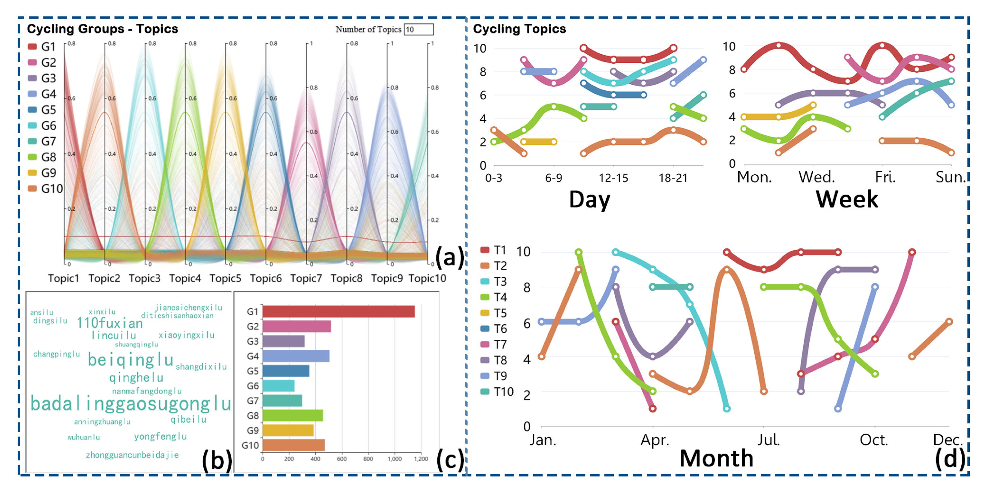
5.2.1. Cycling Grouping and Street Cloud of Cycling Topics

This helps users explore the cycling groups in the city, e.g., how many groups of cyclists in the city and which streets were popular for cyclists and so on. We implemented three interfaces to visually present the inherent details of the cycling groups, namely, cycling groups and topics, the size of the cycling groups and the street cloud of the cycling topics. Among them, the first two were collectively referred to as cycling grouping.

Cycling grouping: In Figure 5b, users can explore the distribution of cycling topics and the relationship between cycling topics and groups. Curves with different colors represent the cyclists in different groups (i.e., $G_c$ from $G1$ to $G10$). Columns from left to right represent the important topics in the corpus (the importance degrees are decreasing), and the vertical axis represents the cyclist’s probability for this topic. Thus, the smooth curves connecting adjacent columns could tell the topic distributions of cyclists, i.e., $T_c$. Such an interface is called a parallel coordinate plot over the topics [43]. Additionally, users know the optimal number of $T_c$ in the input box with a prompt, and they can also change the number in the input box to make a comparison. Moreover, users can also refer to Figure 5c to compare the sizes of different cycling groups.

Street cloud of cycling topics: To examine the specific streets that a cycling group focus on, users can select a group in the left list of Figure 5b, and a corresponding street cloud will appear in Figure 5d. Such a street cloud can visually show the most popular streets of a cycling group, and the distinct font sizes represent their popularity degrees. Moreover, the street cloud is drawn with the same color as the selected group for easy differentiation.

5.2.2. Temporal Evolution of Cycling Topics

This enables users to analyze how cycling topics change over different time granularity.

As shown in Figure 5e, users are able to examine the temporal evolution of cycling topics with a given granularity. The corresponding time unit can be chosen via buttons on the right side, including hours in a day, days in a week, and months in a year. In the evolution interface, the curves with different colors stand for the topics in $T_c$. Users can easily find which topic each curve belongs to through the corresponding colors of different cycling topics on the left. Moreover, the horizontal axis represents continuous time periods, and the vertical axis represents the sorting of topics’ distribution probabilities in a time period (10 represents the highest one). Note that the curve for a topic only connects adjacent time periods when their probabilities exceed the threshold simultaneously. Thus, a curve may break in the middle, such as topic 2 colored in orange in Figure 5e.

5.2.3. Moving Semantics Profiling

This enables users to explore the implicit moving semantics of cycling on roads, e.g., the moving topics of the three moving attributes and the topic distribution of road segments. Moving semantics is visually presented by two interfaces, namely moving topics and moving topic distribution.

Moving topics: The moving attributes studied in this paper include velocity, acceleration and turning angle. Users can select one kind of moving attribute via buttons on the top side. The specific topics are shown in Figure 5g through single-axis scatter diagrams. To be more specific, the same colored circles denote a topic, and the horizontal axis indicates the velocity/acceleration/turning angle values (i.e., a word) for this topic. Moreover, the size of the circle indicates the contribution of the word to the current topic. Hence, users can easily define the meaning of moving topics according to the largest contribution in the topic with different sizes of circles.

Moving topic distribution: When choosing a road segment in Figure 5a, Figure 5f will display the topic distribution of the selected road segment through a ring graph. The colors used in the ring graph are also consistent with those on Figure 5g. With such an interface, users can intuitively find out which topic is the mainstream one for that road segment (e.g., dangerous moving conditions).

Furthermore, after the clustering, road segments in the city are assigned to certain groups (i.e., $G\_s$). In this regard, users are able to further analyze the grouping of different kinds of road segments on the cycling map, which is introduced in the following section.

5.2.4. Cycling Map

This enables users to examine the spatial distribution of cycling semantics on the map, including the cycling topics of cyclists and the moving topics on roads.

For the cycling topics of cyclists, when choosing a group in Figure 5b, streets for its representative topic (e.g., recreational cycling) are shown in Figure 5a. In order to visualize a topic composed of multiple street names precisely, the streets are drawn in the corresponding color in Figure 5b. Moreover, the width of a drawn line is determined by the importance of the street in the given topic. Note that we only delineated the streets above a threshold, i.e., $p\left(w\right|t)>0.015$. With such a visualization, cyclists could easily choose a desirable cycling route according to their preferences.

For the moving topics on roads, when choosing a kind of moving attribute on the top of Figure 5f,g, the grouping of road segments based on the attribute is displayed on the cycling map. Taking velocity as an example, there are four groups corresponding to four extracted topics. Each group is drawn in the color of its representative topic, and the width of the line segments denotes the probability of the topic. Thus, with this interface, users can find out which road segments they are interested in via the color and width of the road segments.

The background in the system was developed by Baidu map (https://lbsyun.baidu.com/index.php?title=jspopularGL, 16 December 2022). Different forms of backgrounds (dark, gray, etc.) could be used to provide visual cues. Moreover, the map provided landmarks such as business districts and scenic spots and also supported any zoom.

6. Case Study

The target users of VizCycSemantics system are cyclists and urban planners. To demonstrate the effectiveness of our visual exploration system for users, we conducted two case studies in Beijing.

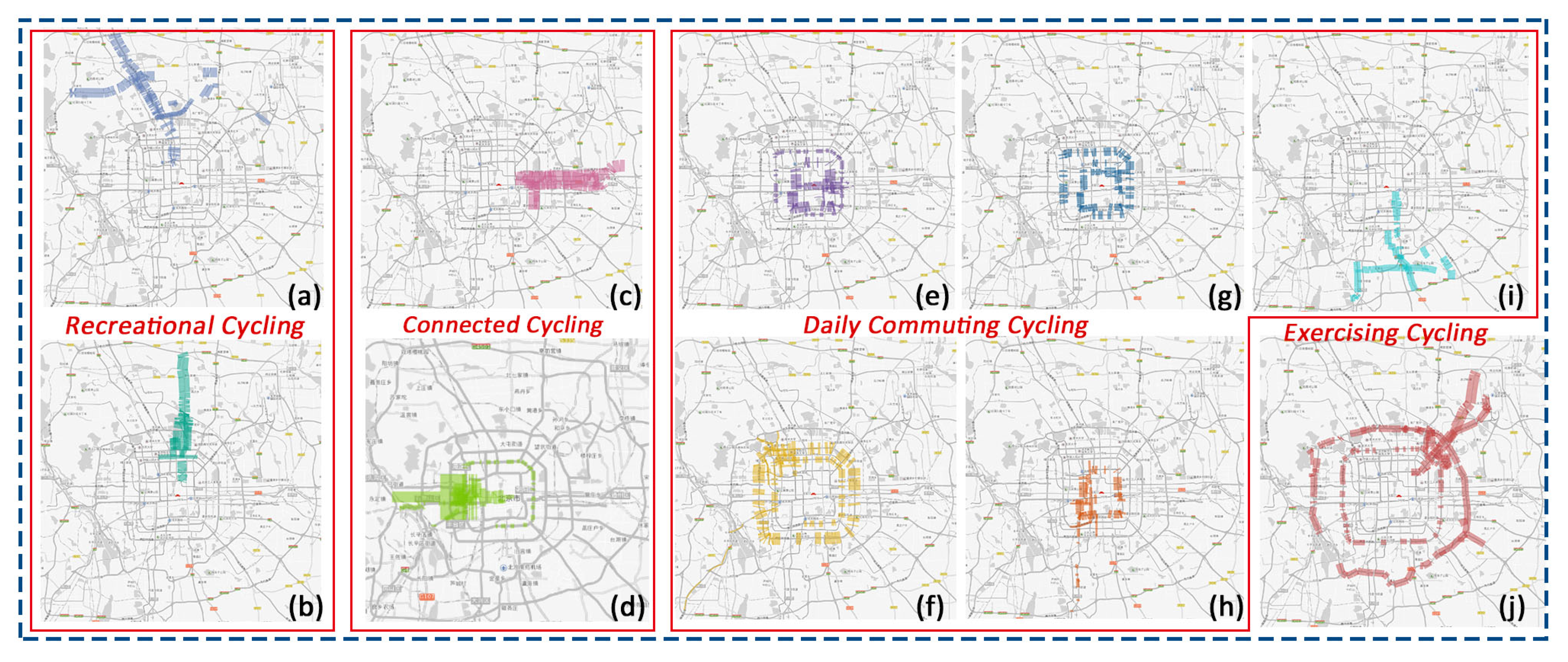
6.1. Case 1: Exploring the Spatiotemporal Patterns of Cycling Themes for Cyclists

We first verified that users could learn about popular group trends and explore the characteristics of the corresponding cycling groups by observing the distribution of topics on the map. First, when users intended to identify the representative cycling groups, they could find a total of 10 cycling topics and 10 cyclist groups obtained through topic extraction and clustering in Figure 6a. Each group had the highest probability on a topic, which represented the main streets that the group often rode on. Then, users could analyze the detailed meaning of each cycling topic through our system. First, users could examine the street names of cycling topics in Figure 6b. Secondly, by zooming on the map, users could view more information within the area around the cycling topics, including the distribution of transportation hubs, office buildings, commercial buildings, residential areas, parks, etc. Therefore, users could define 10 cycling topics and merge the topics with the same definition, and finally obtain four cycling themes, namely recreational cycling, connected cycling, daily commuting cycling and exercising cycling.

6.1.1. Recreational Cycling

There were two groups belonging to the theme of recreational cycling, namely group 4 and group 7. When users wanted to view the geographical distribution of a specific group (e.g., group 4), they could select group 4 in Figure 6a. Then, its spatial distribution of corresponding streets was shown in the cycling map (Figure 7a). Users could find that cyclists in that group mainly rode in the northwest of Beijing. Moreover, when users intended to know the respective street names of the group, they could concentrate on the corresponding street cloud. As shown in (Figure 6b), the Badaling Expressway, Beiqing Road and Qinghe Road are the popular street names of group 4. Qinghe is a famous and beautiful river in Beijing, and the Badaling Expressway is one of the longest and busiest tourist routes with a broad vision from Beijing to Lhasa. Moreover, Qinghe Road is close to the North Garden, Qinghe Bay and Beijing Wenyu River Park. Therefore, the scenery along these roads is pleasant and suitable for recreational cycling. By the same procedure, it could be found that group 7 also referred to a recreational cycling group. Specifically, in Figure 7b, from the center of Beijing along Anli Road and Ansi Road to the north, passing through the Olympic Forest Park and Dongxiaokou Forest Park in the midway, the environment around is delightful. Continuing to ride north, cyclists can enjoy the scenery of Xiaotangshan and other scenic spots. Based on the above analysis, cyclists who would like to ride for recreation can choose the routes in Figure 7a,b to enjoy beautiful scenery.

6.1.2. Connected Cycling

Connected cycling means that cyclists ride for the purpose of connecting transportation, e.g., riding from home to metro stations before taking the metro to working places. The theme incorporated two groups, i.e., group 2 and group 8. As shown in Figure 7c, the two groups passed through the center of Beijing, distributed horizontally. In group 2, most topics were concentrated between the Second Road and Sixth Ring Road in the east of Beijing. In addition, users could find that group 8 passed through West Chang’an Avenue and Fuxingmen Inner Street in the west and going westward until the Sixth Ring Road in Figure 7d. In these areas, there is an entire subway line distributed horizontally, with bus stops evenly distributed along the way. A large number of cyclists may make transfers near the horizontal line. Hence, it is recommended to build more bike-sharing spots near this horizontal traffic line through central Beijing to facilitate traffic.

6.1.3. Daily Commuting Cycling

Groups corresponding to the theme of daily commuting cycling included group 3, group 5, group 9 and group 10, which were active within the Fourth Ring Road (Figure 7e–i). The central area of Beijing is densely distributed with a large number of residence communities, office buildings and business districts. Moreover, the Third Ring Road gathers top enterprises and central institutions, while the Fourth Ring Road is dotted with institutions of higher education and Olympic venues. Hence, residents might use bicycles for daily commuting in the area. Except for the groups distributed in the central area, users could find that group 6 was mainly concentrated in the southeast near the Fifth Ring Road. Note that there are a large number of high-tech businesses and residences, thus indicating a daily commuting cycling as well. Accordingly, for people in the central and southeast area, it is mainstream and convenient to make their daily trips by riding a bicycle. In this respect, more bicycle sharing or public transportation services should be provided in these areas.

6.1.4. Exercising Cycling

As shown in Figure 7j, this theme only included group 1. When users wanted to know how many cyclists were in that group, they could find in Figure 6c that the number of cyclists in group 1 was the largest, obviously exceeding other groups. Cyclists in $group$ 1 often rode along the Fifth Ring Road and the northeast part within the Sixth Ring Road. Additionally, the Fifth Ring Road is long and coherent, and the frontage roads in the northeast to the airport are also long and straight. Moreover, the traffic flow is much less in these roads compared to downtown. Since 2016, there have been several cycling competitions on the Fifth Ring Road and a large number of cyclists are likely to do physical exercise by riding there. Hence, the cycling infrastructures distributed near the Fifth Ring Road can be strengthened suitably to expand the area suitable for exercising cycling. Cyclists looking for exercise and challenge can also choose to ride on the Fifth Ring Road and the frontage roads in the northeast to the airport.

6.1.5. Temporal Evolution of Cycling Topics

When users intended to learn about the evolution of cycling topics at different time scales, they could view the specific changes in the interface of the temporal evolution. As shown in Figure 6d, the probability of each cycling topic changed in a day, a week, and a year, respectively. It can be seen that the cycling topics were time-dependent and mainly changed rapidly. In a day, most topics were mainly concentrated in the working hours (e.g., topics in daily commuting cycling and challenging cycling), and the connected cycling was more active during the morning and evening rush hours. In the week, challenging cycling continued to be active, while recreational cycling was more active on weekends, revealing that some cyclists chose to do leisure cycling at that time. Over the year, the probability of the group fluctuated greatly, and most topics were more inactive during the winter. Hence, users could choose a suitable time to ride.

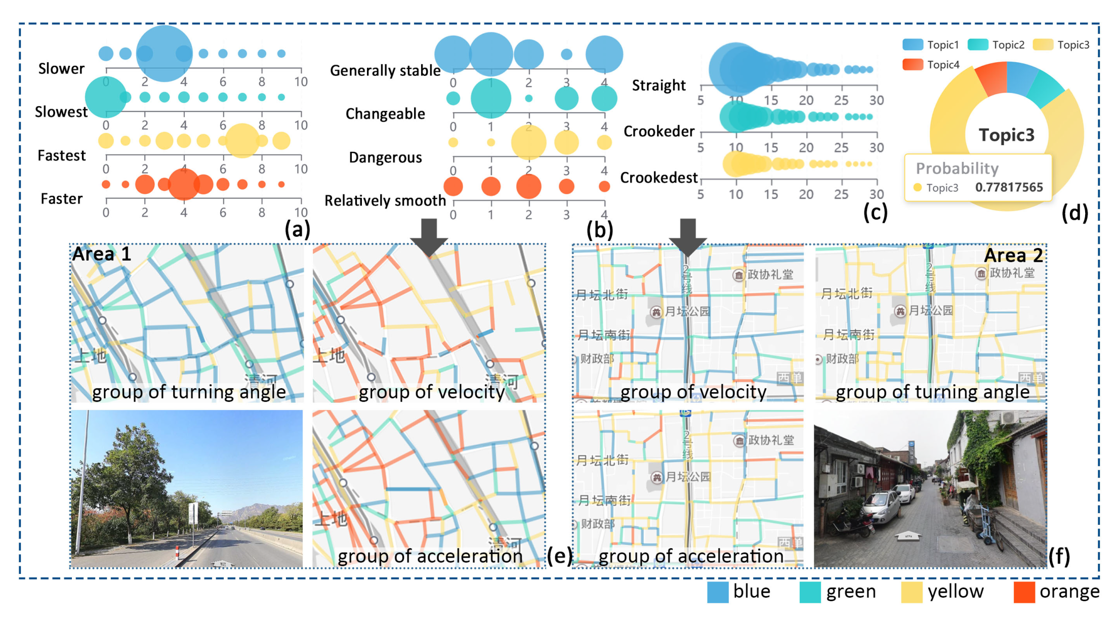
6.2. Case 2: Exploring the Moving Semantics of Road Segments

Finally, we focused on the moving semantics of road segments. First, when users intended to understand the moving characteristic of cycling, they could identify the moving topics based on three moving attributes with our system. For a selected moving attribute, the grouping of each road segment was drawn in the color of its representative topic, and the width of the line segments denoted the probability of the topic. Hence, users could learn about the moving characteristics of cycling on road segments to choose suitable routes for cycling or to find proper locations for cycling planning.

6.2.1. Topics Extracted by Velocity

When selecting the velocity button, users could find information about the topic of velocity with the interface of moving topics. As shown in Figure 8a, according to the largest contribution in the topic, users could extract the primary characteristics of the four topics, namely slower cycling, the slowest cycling, the fastest cycling and faster cycling. The topics were distributed between 0 and 9 $\mathrm{m}/\mathrm{s}$. It can be seen that the probability of slower cycling was the highest, whose velocity was mainly concentrated on 3 $\mathrm{m}/\mathrm{s}$. Moreover, the second topic was the slowest cycling, illustrating that slow cycling was more common within the Sixth Ring Road. Moreover, the third was the fastest cycling (around 7 $\mathrm{m}/\mathrm{s}$), and cyclists could enjoy speedy cycling on the roads with a high proportion in this topic. Furthermore, the probability of faster cycling was the lowest, and its velocities mainly focused on 2–5 $\mathrm{m}/\mathrm{s}$.

Cyclists who would like to ride rapidly can choose the road segments colored by yellow and orange. Additionally, they should try to ride as little as possible on green road segments to avoid traffic jams.

6.2.2. Topics Extracted by Acceleration

As for the acceleration, in Figure 8b, users could summarize the four topics of acceleration as generally stable cycling, changeable cycling, dangerous cycling and relatively smooth cycling. The acceleration responded to the change of velocity, and its distribution of topics was mainly distributed between 0 and 4 $\mathrm{m}/{\mathrm{s}}^2$. Among them, in addition to 4 $\mathrm{m}/{\mathrm{s}}^2$, the first topic mainly focused on 0–2 $\mathrm{m}/{\mathrm{s}}^2$, which meant complicated but generally stable cycling. In addition, changeable cycling conditions were distributed dispersedly, mainly concentrated around 1 $\mathrm{m}/{\mathrm{s}}^2$, 3 $\mathrm{m}/{\mathrm{s}}^2$ and 4 $\mathrm{m}/{\mathrm{s}}^2$, uncovering the instability of cycling. Moreover, the dangerous cycling accelerations were mainly between 2 and 4 $\mathrm{m}/{\mathrm{s}}^2$, which meant that the cycling conditions changed rapidly and emergency acceleration and deceleration occurred. Furthermore, although the distribution of the fourth topic was relatively average, the probability of accelerations decreased from 0 $\mathrm{m}/{\mathrm{s}}^2$ to 4 $\mathrm{m}/{\mathrm{s}}^2$. When the acceleration was 4 $\mathrm{m}/{\mathrm{s}}^2$, the probability was already very small. Thus, we regarded the last topic as relatively smooth cycling.

Road segments colored by blue and orange support relatively stable cycling. Cyclists may enjoy smooth cycling by choosing the area with plenty of blue or orange segments.

6.2.3. Topics Extracted by Turning Angle

To learn about the moving characteristics of the turning angle on road segments, users could view the topics in Figure 8c. The four topics of turning angle were divided into straight cycling, crookeder cycling and crookedest cycling, which were distributed from 10 degrees to 30 degrees. Generally, the probability of 10 degrees was the highest, and it gradually decreased with the increase of the degree of turning angle. Among these topics, the proportion at 10 degrees of straight cycling was the highest, indicating that the number of swerves were the least on the blue segments. Moreover, crookeder cycling and crookedest cycling were more evenly distributed between 10 degrees and 30 degrees than topic 1. Hence, it was easier for more swerves to occur.

Cyclists looking for a safe riding style are advised to ride in the blue area where they are able to enjoy straight cycling.

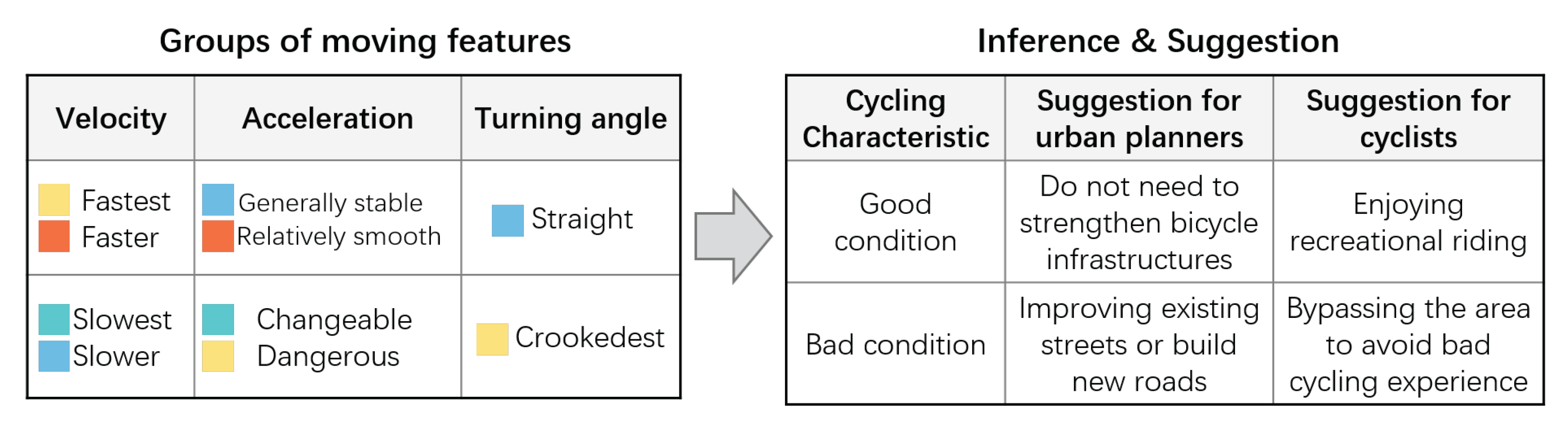
6.2.4. Regional Comparison

We chose two typical areas to analyze whether cycling infrastructure needed to be built or strengthened in the area. Users could compare different roads by moving and zooming in on the map. Area 1 was around the Fifth Ring Road along the Badaling Expressway, where there are mainly residential areas and parks. Area 2 was the western part near the Second Ring Road, with a dense population and concentrated streets.

In area 1, as shown in Figure 8e, the color of the road segments for the velocity was mostly yellow (i.e., the fastest cycling) and orange (i.e., the faster cycling). Taking one road segment colored yellow as an example, as shown in Figure 8d, the distribution probability of this road segment on the four topics was $0.07375018$, $0.07389444$, $0.77817565$ and $0.07417972$, respectively. That is, the fastest cycling had a greater impact. Generally, cyclists can enjoy cycling rapidly in that area. For the acceleration, there were more blue (i.e., generally stable cycling) and orange (i.e., relatively smooth cycling) roads in area 1, indicating that sprint and braking rarely happened in the cycling process and the cycling condition was stable. For the turning angle, roads colored blue (i.e., straight cycling) were more common, thus cyclists tended to ride straightly.

In conclusion, it is shown in the first row of Figure 9 that the riding in area 1 is good. Along the Badaling Expressway, there are a lot of frontage roads suitable for cycling. In addition, recreational riding in case 1 also passes through this area. Residents living here can ride conveniently, and the area is also developed into a popular choice for cycling enthusiasts. Hence, the bicycle infrastructures in the area do not need to be strengthened.

In area 2, it is shown in Figure 8f that the velocity grouping was mainly blue (i.e., the slower cycling) and green (i.e., the slowest cycling). For the acceleration, the color of the grouping was mainly yellow (i.e., dangerous cycling) and green (i.e., changeable cycling), indicating that the cycling in area 2 was not stable. For the turning angle, most roads were obviously yellow, revealing that cyclists rode crookedly.

It is summarized in the second row of Figure 9 that riding in area 2 is bad, so the construction of bicycle infrastructure is necessary. Cyclists can bypass the area to avoid degrading their cycling experience. Urban planners can better improve existing streets or build new roads.

7. Conclusions and Future Work

This work proposed an interactive visualization system named VizCycSemantics for the exploration of cycling semantics, and the users of our system were mainly cyclists and urban planners. Based on large-scale GPS trajectories and road network data, the semantics studied in the paper were twofold, namely, the behavior semantics of cyclists and the moving semantics on road segments. Specifically, trajectories were converted into a street name corpus for cyclists and a moving feature corpus for road segments, respectively. Then, we used an LDA model to automatically extract the cyclists’ behavior semantic (i.e., cycling topics of cyclists) and moving semantics (i.e., moving topics on roads). We further employed the k-means++ algorithm to capture the groups of similar cyclists and road segments in the city. At last, multiple user interfaces were implemented to visualize the various patterns of cycling semantics. To better demonstrate the practicality of the system in transportation planning, two case studies were shown within the Sixth Ring Road in Beijing. First, with specific cycling topics shown in our system, cyclists could find popular group trends and suitable routes of their own interest. Urban planners could also make corresponding traffic plans through different cycling topics. Secondly, with the moving topics on road segments, cyclists could choose routes with fast, stable and straight cycling. Urban planner could find out where the cycling infrastructures should be built/improved via the types of moving conditions in the area. Moreover, this system only employed some very basic information from the trajectory and road network data, thus it could be easily and safely generalized to other cities.

In future work, we will broaden and deepen the cycling semantics exploration from more perspectives. For example, the visited points of interests (POIs) can be considered as words in the process of trajectory textualization, so as to import human activity semantics. Furthermore, social media data can be considered to enhance trajectory semantics and obtain a richer knowledge. It is also a good idea to make our own cycling trajectories with a camera, which can provide more contextual information to enrich cycling semantics. Additionally, we intend to refine the visualizations to further enhance the aesthetics of and interaction with the system, enabling users to do more diverse and personalized analysis and exploration.

References

- Boss, D.; Nelson, T.; Winters, M.; Ferster, C.J. Using crowdsourced data to monitor change in spatial patterns of bicycle ridership. J. Transp. Health 2018, 9, 226–233. [Google Scholar] [CrossRef]
- Brauer, A.; Mäkinen, V.; Oksanen, J. Characterizing cycling traffic fluency using big mobile activity tracking data. Comput. Environ. Urban Syst. 2021, 85, 101553. [Google Scholar] [CrossRef]
- Commonwealth of Australia. National Road Safety Action Plan 2021–30. 2021. Available online: https://www.roadsafety.gov.au/sites/default/files/documents/National-Road-Safety-Strategy-2021-30.pdf (accessed on 15 September 2020).
- Ministry of Transport in China. Guidelines of the Ministry of Transport and Other 10 Departments on Encouraging and Regulating the Development of Internet Bike Rental. 2017. Available online: https://www.mot.gov.cn/yijianzhengji/201705/P020170521640994522102.doc (accessed on 15 September 2020).
- U.S. Department of Transportation. Encourage and Promote Safe Bicycling and Walking.; 2019. Available online: https://www.transportation.gov/mission/health/Encourage-and-Promote-Safe-Bicycling-and-Walking (accessed on 16 September 2020).
- Chu, D.; Sheets, D.A.; Zhao, Y.; Wu, Y.; Yang, J.; Zheng, M.; Chen, G. Visualizing hidden themes of taxi movement with semantic transformation. In Proceedings of the 2014 IEEE Pacific Visualization Symposium, Yokohama, Japan, 4–7 March 2014; pp. 137–144. [Google Scholar]
- Beecham, R.; Wood, J. Characterising group-cycling journeys using interactive graphics. Transp. Res. Part C Emerg. Technol. 2014, 47, 194–206. [Google Scholar] [CrossRef] [Green Version]
- Kassim, A.; Tayyeb, H.; Al-Falahi, M. Critical review of cyclist speed measuring techniques. J. Traffic Transp. Eng. (Engl. Ed.) 2020, 7, 98–110. [Google Scholar] [CrossRef]
- Al-Kodmany, K. Bridging the gap between technical and local knowledge: Tools for promoting community-based planning and design. J. Archit. Plan. Res. 2001, 18, 110–130. [Google Scholar]
- Chen, W.; Huang, Z.; Wu, F.; Zhu, M.; Guan, H.; Maciejewski, R. Vaud: A visual analysis approach for exploring spatio-temporal urban data. IEEE Trans. Vis. Comput. Graph. 2018, 24, 2636–2648. [Google Scholar] [CrossRef]
- Liao, C.; Chen, C.; Zhang, Z.; Xie, H. Understanding and visualizing passengers’ travel behaviours: A device-free sensing way leveraging taxi trajectory data. Pers. Ubiquitous Comput. 2019, 26, 491–503. [Google Scholar] [CrossRef]
- He, J.; Chen, H.; Chen, Y.; Tang, X.; Zou, Y. Diverse visualization techniques and methods of moving-object-trajectory data: A review. ISPRS Int. J. Geo-Inf. 2019, 8, 63. [Google Scholar] [CrossRef] [Green Version]
- Kreso, I.; Kapo, A.; Turulja, L. Data mining privacy preserving: Research agenda. Wiley Interdiscip. Rev. Data Min. Knowl. Discov. 2021, 11, e1392. [Google Scholar] [CrossRef]
- Chen, C.; Zhang, D.; Castro, P.S.; Li, N.; Sun, L.; Li, S.; Wang, Z. iBOAT: Isolation-based online anomalous trajectory detection. IEEE Trans. Intell. Transp. Syst. 2013, 14, 806–818. [Google Scholar] [CrossRef]
- Chen, C.; Zhang, D.; Ma, X.; Guo, B.; Wang, L.; Wang, Y.; Sha, E. Crowddeliver: Planning city-wide package delivery paths leveraging the crowd of taxis. IEEE Trans. Intell. Transp. Syst. 2016, 18, 1478–1496. [Google Scholar] [CrossRef]
- Chen, C.; Jiao, S.; Zhang, S.; Liu, W.; Feng, L.; Wang, Y. TripImputor: Real-time imputing taxi trip purpose leveraging multi-sourced urban data. IEEE Trans. Intell. Transp. Syst. 2018, 19, 3292–3304. [Google Scholar] [CrossRef]
- Chen, C.; Ding, Y.; Xie, X.; Zhang, S.; Wang, Z.; Feng, L. TrajCompressor: An online map-matching-based trajectory compression framework leveraging vehicle heading direction and change. IEEE Trans. Intell. Transp. Syst. 2019, 21, 2012–2028. [Google Scholar] [CrossRef]
- Chen, C.; Yang, S.; Wang, Y.; Guo, B.; Zhang, D. CrowdExpress: A probabilistic framework for on-time crowdsourced package deliveries. IEEE Trans. Big Data 2020, 8, 827–842. [Google Scholar] [CrossRef]
- Chen, C.; Liu, Q.; Wang, X.; Liao, C.; Zhang, D. semi-Traj2Graph Identifying Fine-Grained Driving Style With GPS Trajectory Data via Multi-Task Learning. IEEE Trans. Big Data 2021, 8, 1550–1565. [Google Scholar] [CrossRef]
- Andrienko, G.; Andrienko, N.; Chen, W.; Maciejewski, R.; Zhao, Y. Visual analytics of mobility and transportation: State of the art and further research directions. IEEE Trans. Intell. Transp. Syst. 2017, 18, 2232–2249. [Google Scholar] [CrossRef]
- Chen, W.; Guo, F.; Wang, F.Y. A survey of traffic data visualization. IEEE Trans. Intell. Transp. Syst. 2015, 16, 2970–2984. [Google Scholar] [CrossRef]
- Kraak, M.J. The space-time cube revisited from a geovisualization perspective. In Proceedings of the 21st International Cartographic Conference, Citeseer, Durban, South Africa, 10–16 August 2003; pp. 1988–1996. [Google Scholar]
- Bach, B.; Dragicevic, P.; Archambault, D.; Hurter, C.; Carpendale, S. A descriptive framework for temporal data visualizations based on generalized space-time cubes. Comput. Graph. Forum 2017, 36, 36–61. [Google Scholar] [CrossRef] [Green Version]
- Wang, Z.; Ye, T.; Lu, M.; Yuan, X.; Qu, H.; Yuan, J.; Wu, Q. Visual exploration of sparse traffic trajectory data. IEEE Trans. Vis. Comput. Graph. 2014, 20, 1813–1822. [Google Scholar] [CrossRef]
- Shamal, A.D.; Zhao, Y.; Kamw, F.; Yang, J.; Ye, X.; Chen, W. QuteVis: Visually studying transportation patterns using multisketch query of joint traffic situations. IEEE Comput. Graph. Appl. 2019, 41, 35–48. [Google Scholar]
- Krüger, R.; Simeonov, G.; Beck, F.; Ertl, T. Visual interactive map matching. IEEE Trans. Vis. Comput. Graph. 2018, 24, 1881–1892. [Google Scholar] [CrossRef]
- Lu, M.; Lai, C.; Ye, T.; Liang, J.; Yuan, X. Visual analysis of multiple route choices based on general gps trajectories. IEEE Trans. Big Data 2017, 3, 234–247. [Google Scholar] [CrossRef]
- Kamw, F.; Al-Dohuki, S.; Zhao, Y.; Eynon, T.; Sheets, D.; Yang, J.; Ye, X.; Chen, W. Urban structure accessibility modeling and visualization for joint spatiotemporal constraints. IEEE Trans. Intell. Transp. Syst. 2019, 21, 104–116. [Google Scholar] [CrossRef]
- Itoh, M.; Yokoyama, D.; Toyoda, M.; Tomita, Y.; Kawamura, S.; Kitsuregawa, M. Visual exploration of changes in passenger flows and tweets on mega-city metro network. IEEE Trans. Big Data 2016, 2, 85–99. [Google Scholar] [CrossRef]
- Zeng, W.; Fu, C.W.; Arisona, S.M.; Schubiger, S.; Burkhard, R.; Ma, K.L. Visualizing the relationship between human mobility and points of interest. IEEE Trans. Intell. Transp. Syst. 2017, 18, 2271–2284. [Google Scholar] [CrossRef]
- Zhao, X.; Zhang, Y.; Hu, Y.; Wang, S.; Li, Y.; Qian, S.; Yin, B. Interactive visual exploration of human mobility correlation based on smart card data. IEEE Trans. Intell. Transp. Syst. 2020, 22, 4825–4837. [Google Scholar] [CrossRef]
- Shi, Y.; Liu, Y.; Tong, H.; He, J.; Yan, G.; Cao, N. Visual analytics of anomalous user behaviors: A survey. IEEE Trans. Big Data 2020, 8, 377–396. [Google Scholar] [CrossRef] [Green Version]
- Feng, Z.; Li, H.; Zeng, W.; Yang, S.H.; Qu, H. Topology density map for urban data visualization and analysis. IEEE Trans. Vis. Comput. Graph. 2020, 27, 828–838. [Google Scholar] [CrossRef]
- Al-Dohuki, S.; Wu, Y.; Kamw, F.; Yang, J.; Li, X.; Zhao, Y.; Ye, X.; Chen, W.; Ma, C.; Wang, F. Semantictraj: A new approach to interacting with massive taxi trajectories. IEEE Trans. Vis. Comput. Graph. 2016, 23, 11–20. [Google Scholar] [CrossRef]
- Bahmani, B.; Moseley, B.; Vattani, A.; Kumar, R.; Vassilvitskii, S. Scalable k-means++. arXiv 2012, arXiv:1203.6402. [Google Scholar] [CrossRef]
- Lou, Y.; Zhang, C.; Zheng, Y.; Xie, X.; Wang, W.; Huang, Y. Map-matching for low-sampling-rate GPS trajectories. In Proceedings of the 17th ACM SIGSPATIAL International Conference on Advances in Geographic Information Systems, Seattle, WA, USA, 4–6 November 2009; pp. 352–361. [Google Scholar]
- Jiang, L.; Chen, C.X.; Chen, C. L2MM: Learning to Map Matching with Deep Models for Low-Quality GPS Trajectory Data. ACM Trans. Knowl. Discov. Data (TKDD) 2022, 17, 39. [Google Scholar] [CrossRef]
- Newson, P.; Krumm, J. Hidden Markov map matching through noise and sparseness. In Proceedings of the 17th ACM SIGSPATIAL International Conference on Advances in Geographic Information Systems, Seattle, WA, USA, 4–6 November 2009; pp. 336–343. [Google Scholar]
- Ryan, M.S.; Nudd, G.R. The Viterbi Algorithm; University of Warwick: Coventry, UK, 1993. [Google Scholar]
- Zheng, Y.; Li, Q.; Chen, Y.; Xie, X.; Ma, W.Y. Understanding mobility based on GPS data. In Proceedings of the 10th International Conference on Ubiquitous Computing, Seoul, Republic of Korea, 21–24 September 2008; pp. 312–321. [Google Scholar]
- Blei, D.M.; Ng, A.Y.; Jordan, M.I. Latent dirichlet allocation. J. Mach. Learn. Res. 2003, 3, 993–1022. [Google Scholar]
- Yuan, C.; Yang, H. Research on K-value selection method of K-means clustering algorithm. J 2019, 2, 226–235. [Google Scholar] [CrossRef] [Green Version]
- Dou, W.; Wang, X.; Chang, R.; Ribarsky, W. Paralleltopics: A probabilistic approach to exploring document collections. In Proceedings of the 2011 IEEE Conference on Visual Analytics Science and Technology (VAST), Providence, RI, USA, 23–28 October 2011; pp. 231–240. [Google Scholar]
Disclaimer/Publisher’s Note: The statements, opinions and data contained in all publications are solely those of the individual author(s) and contributor(s) and not of MDPI and/or the editor(s). MDPI and/or the editor(s) disclaim responsibility for any injury to people or property resulting from any ideas, methods, instructions or products referred to in the content. |
© 2023 by the authors. Licensee MDPI, Basel, Switzerland. This article is an open access article distributed under the terms and conditions of the Creative Commons Attribution (CC BY) license (https://creativecommons.org/licenses/by/4.0/).
Share and Cite
Gao, X.; Liao, C.; Chen, C.; Li, R. Visual Exploration of Cycling Semantics with GPS Trajectory Data. Appl. Sci. 2023, 13, 2748. https://doi.org/10.3390/app13042748
Gao X, Liao C, Chen C, Li R. Visual Exploration of Cycling Semantics with GPS Trajectory Data. Applied Sciences. 2023; 13(4):2748. https://doi.org/10.3390/app13042748
Chicago/Turabian StyleGao, Xuansu, Chengwu Liao, Chao Chen, and Ruiyuan Li. 2023. "Visual Exploration of Cycling Semantics with GPS Trajectory Data" Applied Sciences 13, no. 4: 2748. https://doi.org/10.3390/app13042748