
Sep-RefineNet: A Deinterleaving Method for Radar Signals Based on Semantic Segmentation

Abstract
:1. Introduction
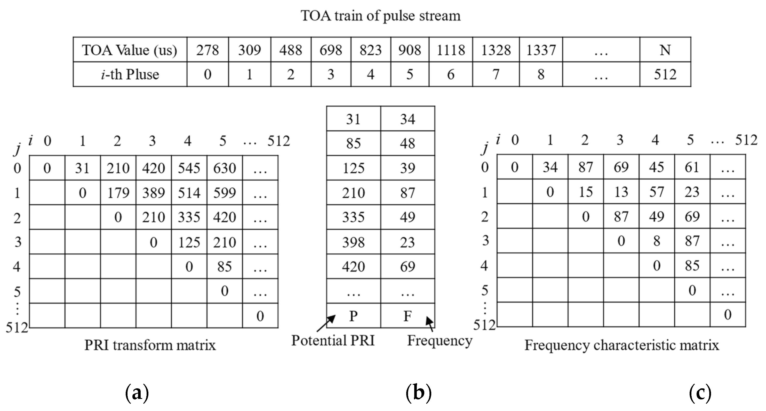
- An FCM is designed to encode and decode the PRI of radar pulse signals. It encodes different PRI’s semantic information into the FCM.
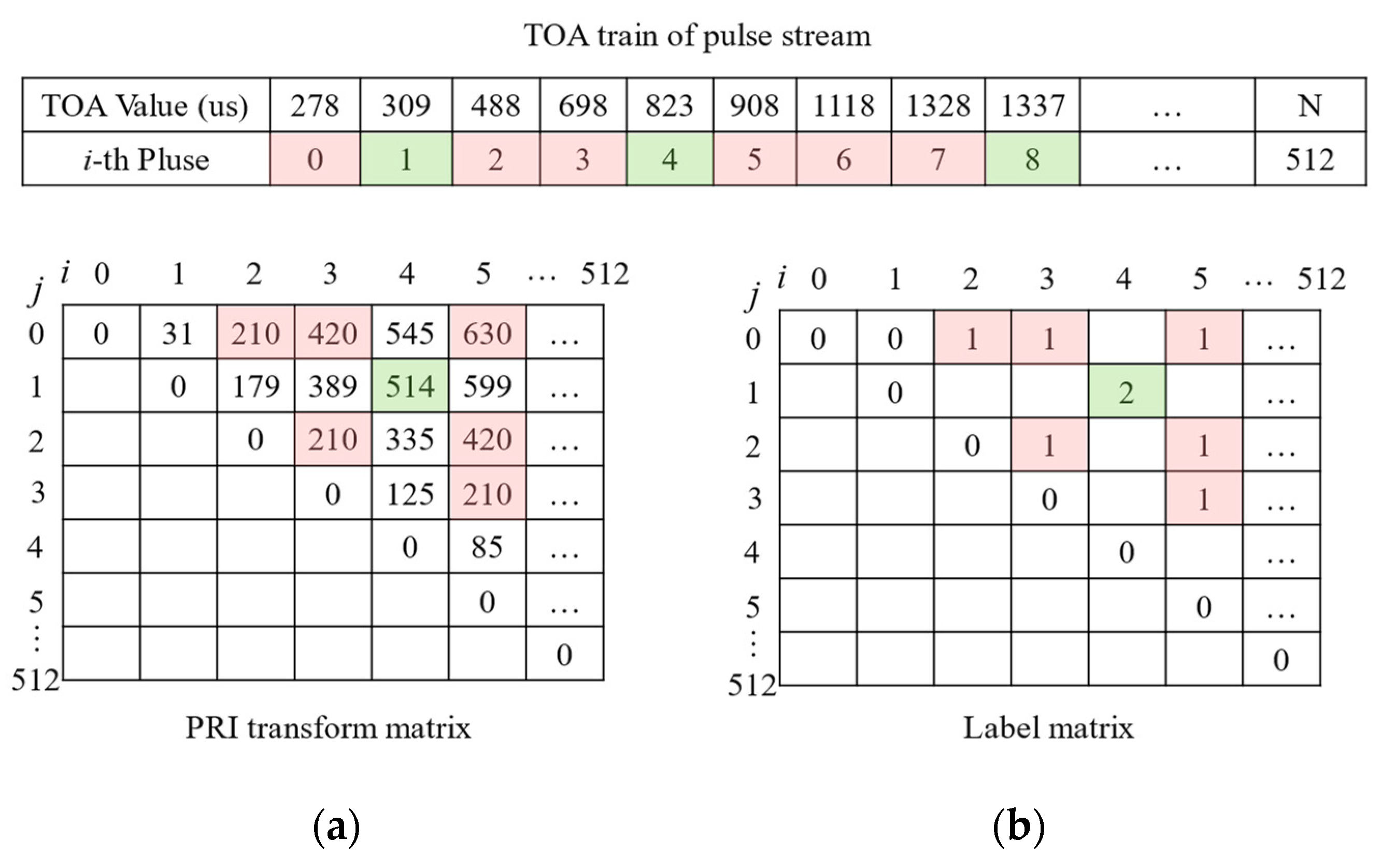
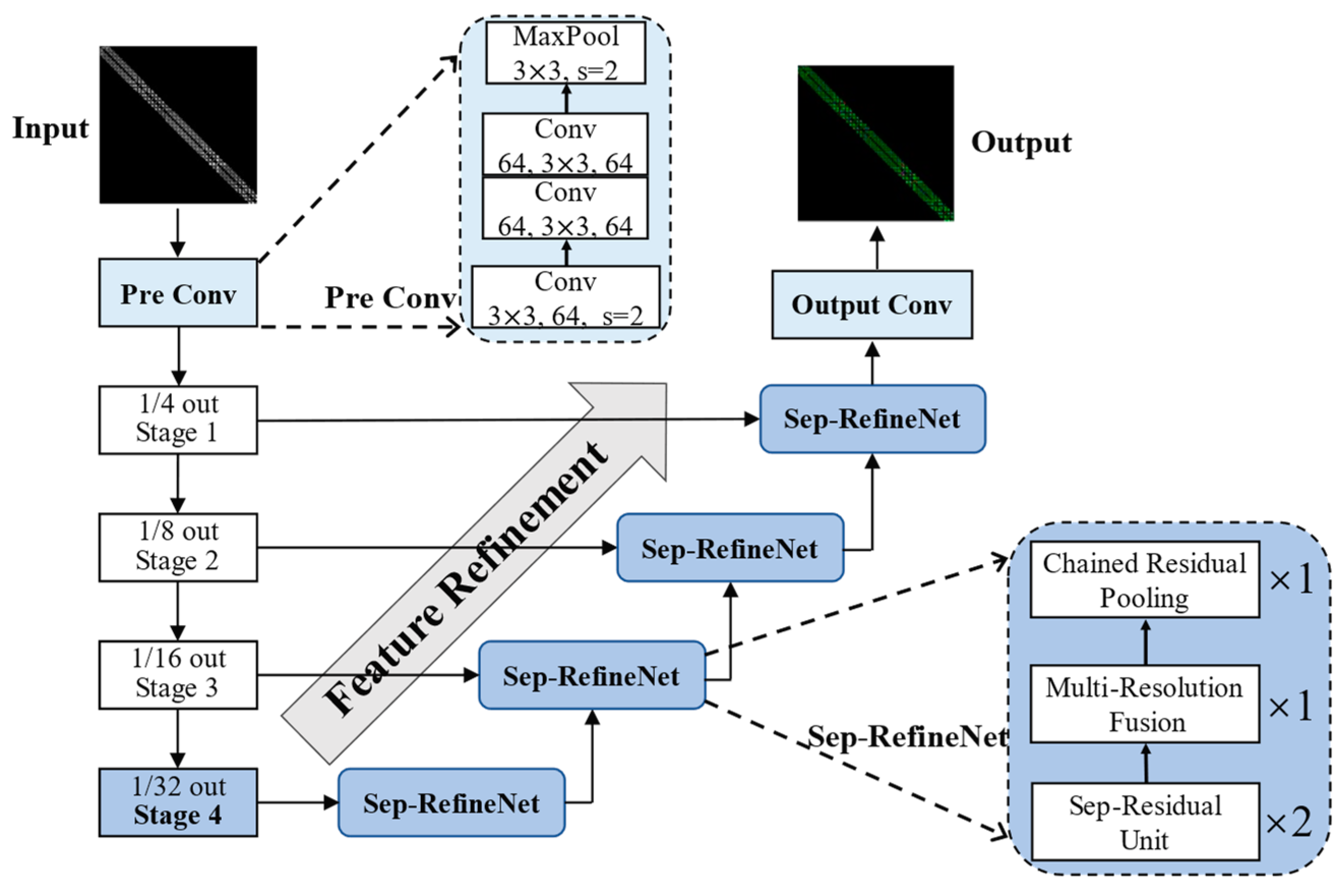
- A multi-receptive field and multi-channel separation semantic segmentation network named Sep-RefineNet is used to learn the semantic features of the FCM. Through position decoding, the deinterleaving algorithm is made more intelligent, reducing the dependence on manual experience parameters.
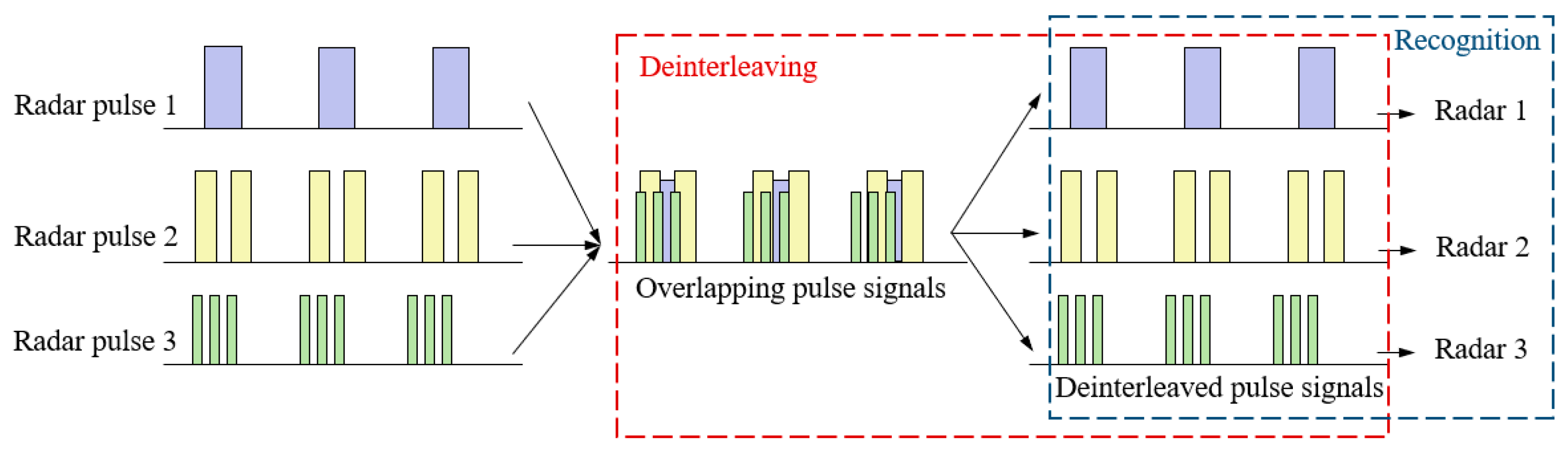
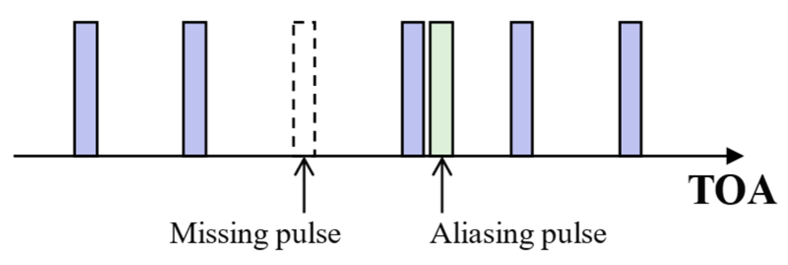
- Under the influence of aliasing pluses and missing pluses, it can sort constant PRI, staggered PRI, and jittered PRI, and improve the robustness and accuracy of the deinterleaving.
2. Related Work
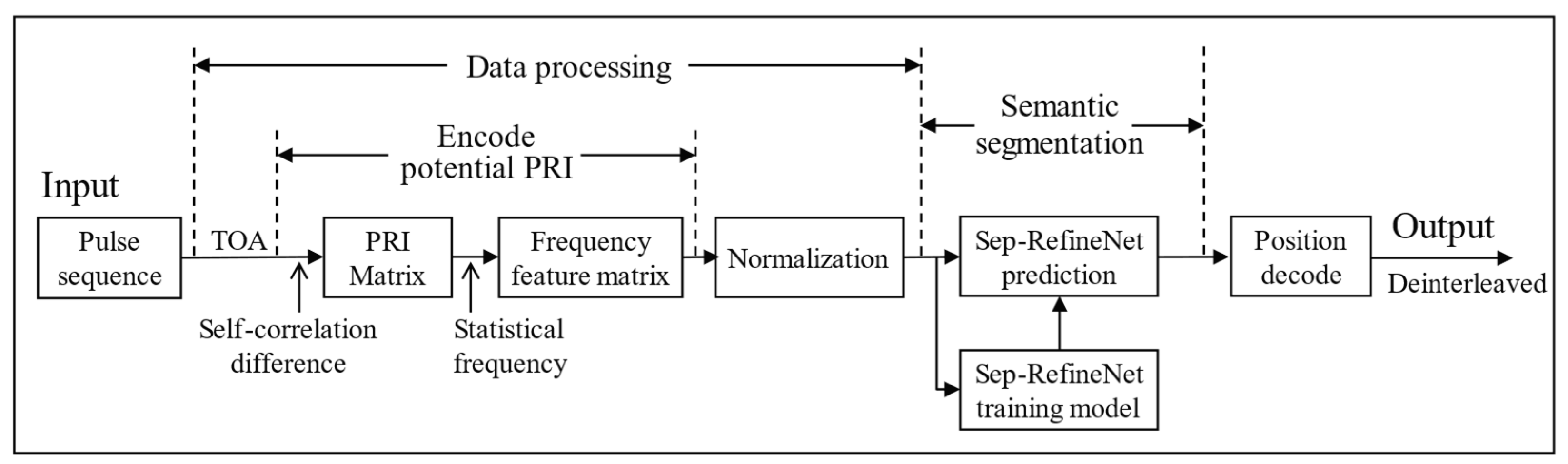
3. System Framework and Method
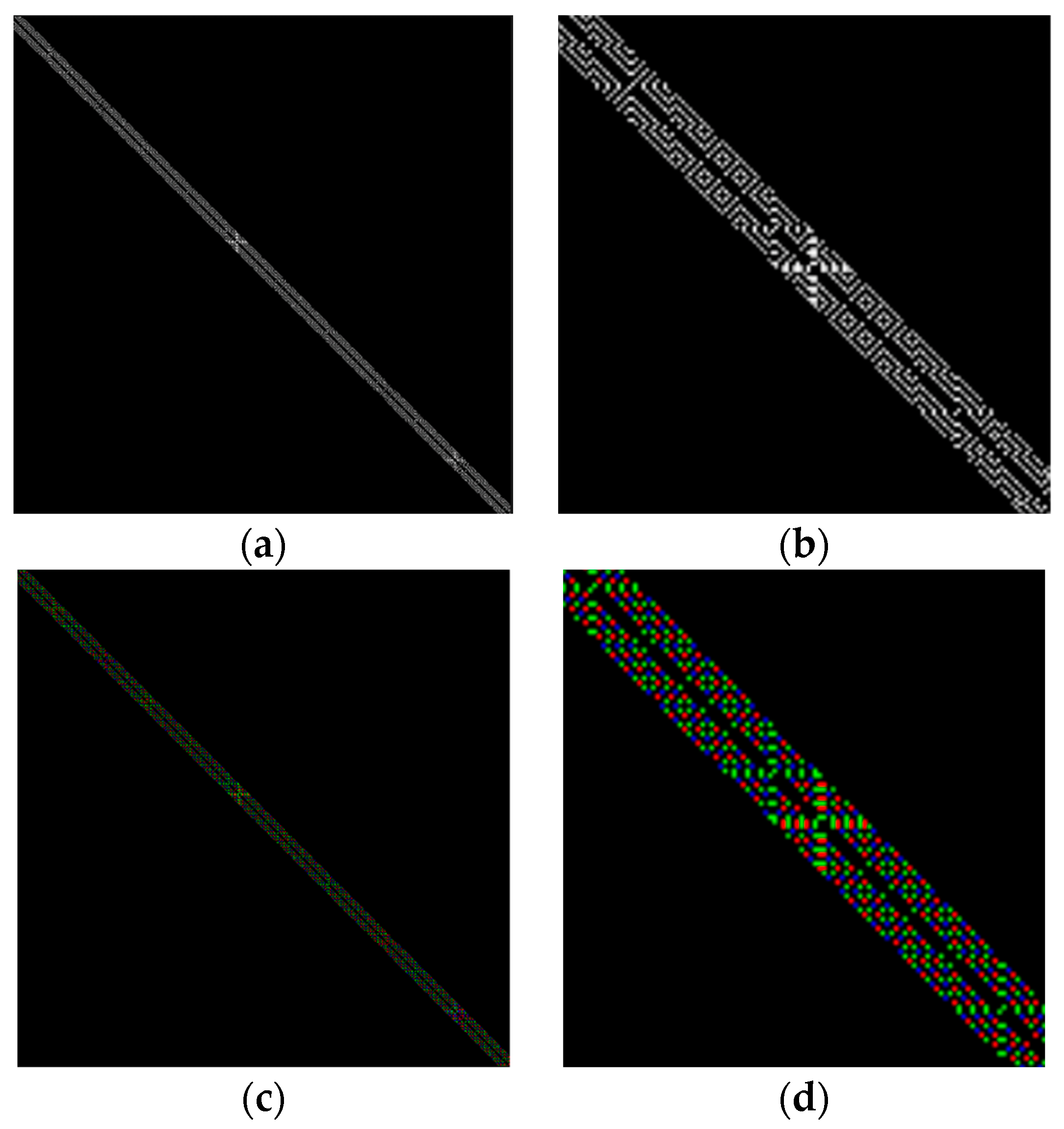
3.1. Frequency Characteristic Matrix
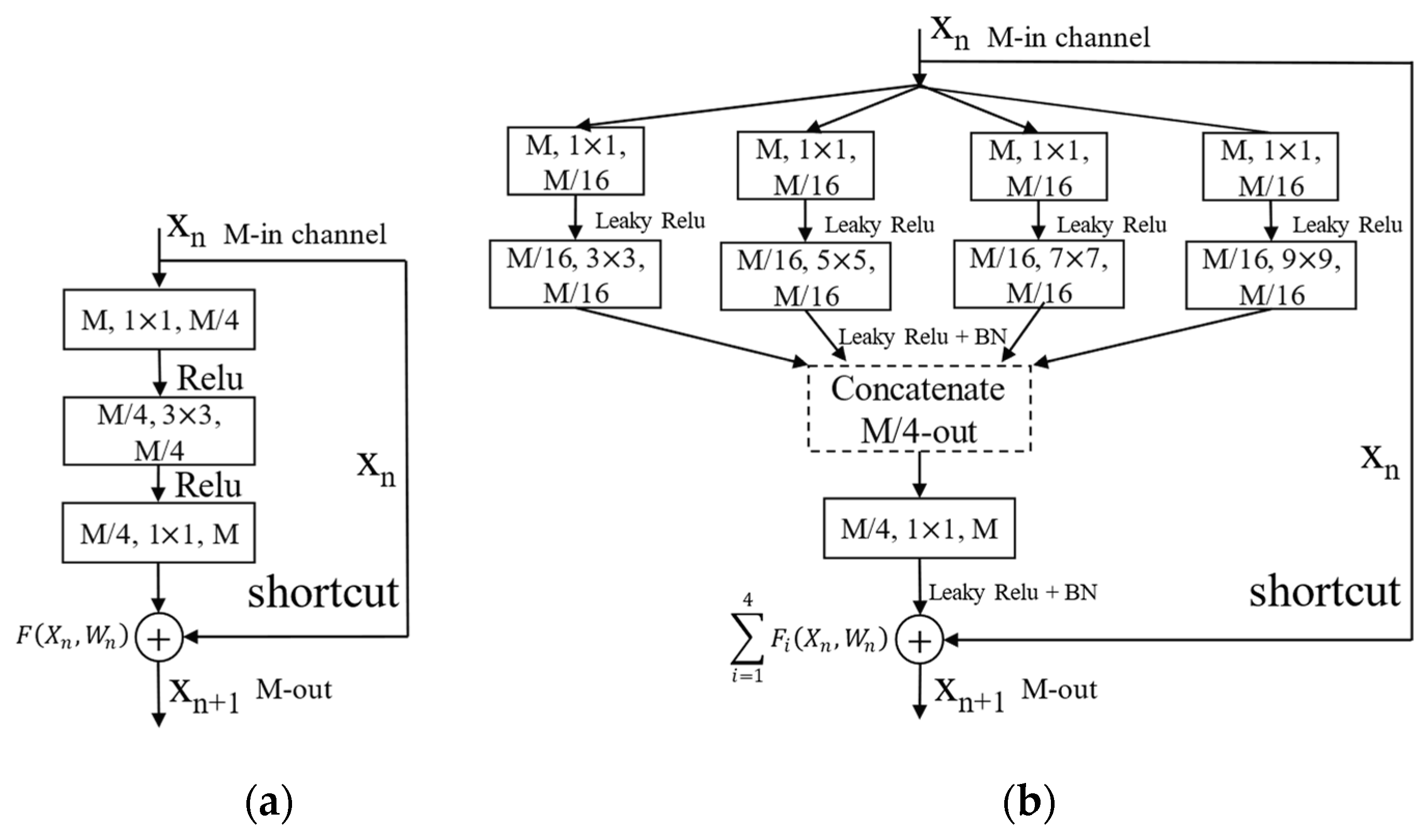
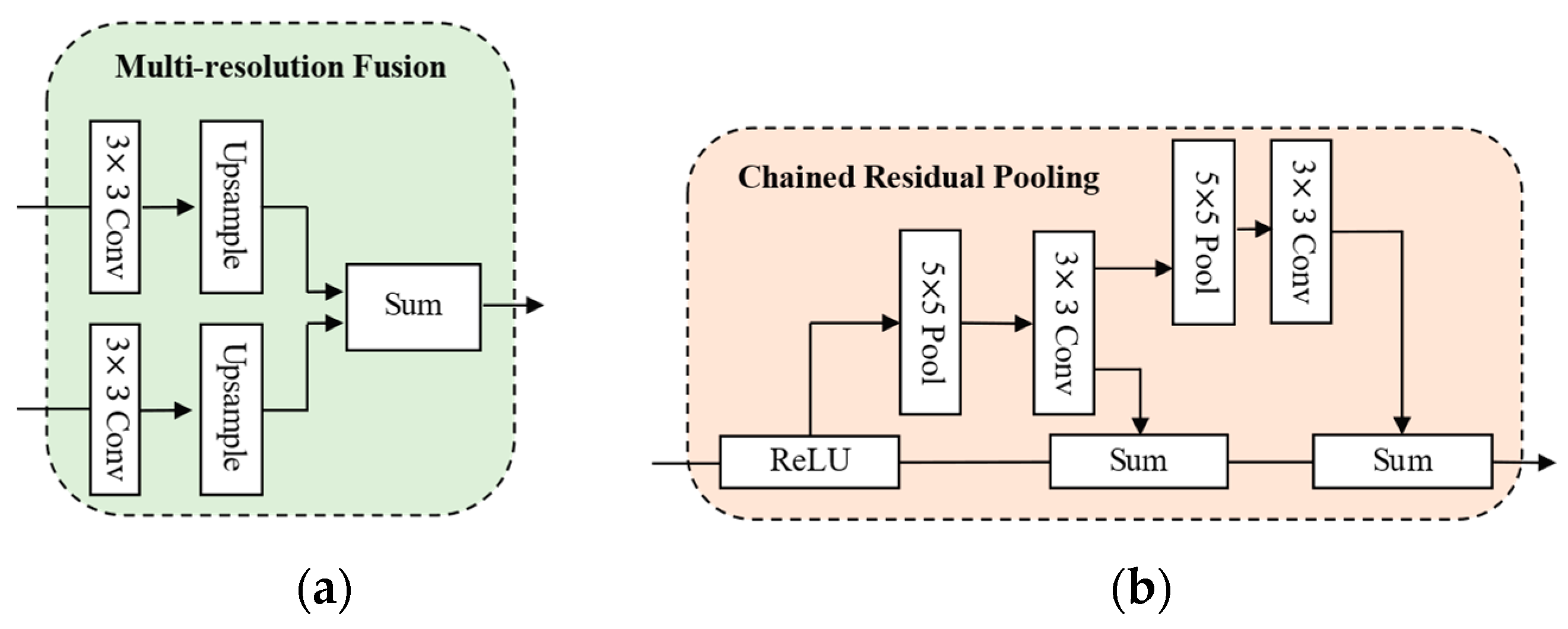
3.2. Sep-RefineNet
4. Experimental Results and Discussion
4.1. Experimental Dataset
4.2. Experimental Results
4.2.1. Verify the Effectiveness of Sep-RefineNet
4.2.2. Verify the Effectiveness of Deinterleaving
4.2.3. Verify the Anti-Noise Ability
5. Conclusions
Author Contributions
Funding
Institutional Review Board Statement
Informed Consent Statement
Data Availability Statement
Conflicts of Interest
Abbreviations
| PDW | pulse description words |
| PRI | pulse repetition interval |
| TOA | time of arrival |
| FCM | frequency characteristic matrix |
| TM | transformation matrix |
| Sep-RefineNet | separable refinement network |
| SRU | Sep-Residual unit |
| FL | focal loss |
| LR | learning rate |
References
- Gupta, M.; Hareesh, G.; Mahla, A.K. Electronic Warfare: Issues and Challenges for Emitter Classification. Def. Sci. J. 2011, 61, 228–234. [Google Scholar] [CrossRef] [Green Version]
- Chen, L.; Ma, Q.; Luo, S.S.; Ye, F.J.; Cui, H.Y.; Cui, T.J. Touch-Programmable Metasurface for Various Electromagnetic Manipulations and Encryptions. Small 2022, 18, 2203871. [Google Scholar] [CrossRef] [PubMed]
- Ma, Q.; Bai, G.D.; Jing, H.B.; Yang, C.; Li, L.; Cui, T.J. Smart Metasurface with Self-Adaptively Reprogrammable Functions. Light Sci. Appl. 2019, 8, 98. [Google Scholar] [CrossRef] [PubMed] [Green Version]
- Latombe, G.; Granger, E.; Dilkes, F.A. Fast Learning of Grammar Production Probabilities in Radar Electronic Support. IEEE Trans. Aerosp. Electron. Syst. 2010, 46, 1262–1289. [Google Scholar] [CrossRef]
- Liu, Q.; Zheng, S.; Zuo, Y.; Zhang, H.; Liu, J. Electromagnetic Environment Effects and Protection of Complex Electronic Information Systems. In Proceedings of the 2020 IEEE MTT-S International Conference on Numerical Electromagnetic and Multiphysics Modeling and Optimization (NEMO), Hangzhou, China, 7–9 December 2020; pp. 1–4. [Google Scholar]
- Jinping, S.; Zhen, L.; Li, L.; Xiang, L. Progress in Radar Emitter Signal Deinterleaving. J. Radars 2022, 11, 418–433. [Google Scholar] [CrossRef]
- Saperstein, S.; Campbell, J.W. Signal Recognition in a Complex Radar Environment. Electronic 1977, 3, 8. [Google Scholar]
- Jiegui, W.; Xueming, J. Survey on deinterleaving technique for modern radar signal. Radar Sci. Technol. 2006, 4, 104–108. [Google Scholar] [CrossRef]
- Nishiguchi, K.; Kobayashi, M. Improved Algorithm for Estimating Pulse Repetition Intervals. IEEE Trans. Aerosp. Electron. Syst. 2000, 36, 407–421. [Google Scholar] [CrossRef]
- Kok, E.H.; Turkmen, L.E.; Unsal, S. Electronic Warfare Support Measures (ESM) Subsystem Model in a Simulated Tactical Environment. In Proceedings of the 2006 IEEE 14th Signal Processing and Communications Applications, Antalya, Turkey, 17–19 April 2006; pp. 1–4. [Google Scholar]
- Jian, M.; Laizhao, H. Repetitive cycle transform for signal processing. Electron. Inf. Warf. Technol. 1998, 13, 1–7. [Google Scholar]
- Mingsong, L. Research on Interpulse Parameter Sorting of Radar Signal Based on Machine Learning. Master Dissertation, Harbin Engineering University, Harbin, China, 2021. [Google Scholar] [CrossRef]
- Mardia, H.K. New Techniques for the Deinterleaving of Repetitive Sequences. IEE Proc. F Radar Signal Process. UK 1989, 136, 149. [Google Scholar] [CrossRef]
- Milojević, D.J.; Popović, B.M. Improved Algorithm for the Deinterleaving of Radar Pulses. IEE Proc. F (Radar Signal Process.) 1992, 139, 98–104. [Google Scholar] [CrossRef]
- Liu, Y.; Zhang, Q. Improved Method for Deinterleaving Radar Signals and Estimating PRI Values. IET Radar Sonar Navig. 2018, 12, 506–514. [Google Scholar] [CrossRef]
- Xin, G.; Hangping, Z. An improved algorithm PRI transform based on coherence of time delay sequence. Radar Sci. Technol. 2018, 16, 49–54. [Google Scholar] [CrossRef]
- Wengui, Z.; Kai, L.; Jiabin, H. Sorting of the aliasing LFM radar signals based on PRI transform. Radar Sci. Technol. 2016, 14, 630–634. [Google Scholar] [CrossRef]
- Ying, F.; Xing, W. Radar Signal Recognition Based on Modified Semi-Supervised SVM Algorithm. In Proceedings of the 2017 IEEE 2nd Advanced Information Technology, Electronic and Automation Control Conference (IAEAC), Chongqing, China, 25–26 March 2017; pp. 2336–2340. [Google Scholar]
- Wei, S.; Qu, Q.; Su, H.; Wang, M.; Shi, J.; Hao, X. Intra-Pulse Modulation Radar Signal Recognition Based on CLDN Network. IET Radar Sonar Navig. 2020, 14, 803–810. [Google Scholar] [CrossRef]
- Qu, Z.; Hou, C.; Hou, C.; Wang, W. Radar Signal Intra-Pulse Modulation Recognition Based on Convolutional Neural Network and Deep Q-Learning Network. IEEE Access 2020, 8, 49125–49136. [Google Scholar] [CrossRef]
- Ning, B. Radar Signal Sorting Method Based on Neural Network. Master’s Thesis, Xidian University, Xi’an, China, 2019. [Google Scholar] [CrossRef]
- Li, X.; Liu, Z.; Huang, Z. Attention-Based Radar PRI Modulation Recognition With Recurrent Neural Networks. IEEE Access 2020, 8, 57426–57436. [Google Scholar] [CrossRef]
- He, K.; Zhang, X.; Ren, S.; Sun, J. Deep Residual Learning for Image Recognition. In Proceedings of the 2016 IEEE Conference on Computer Vision and Pattern Recognition (CVPR), Las Vegas, NV, USA, 27–30 June 2016; pp. 770–778. [Google Scholar]
- Santurkar, S.; Tsipras, D.; Ilyas, A.; Madry, A. How does batch normalization help optimization? arXiv 2019, arXiv:1805.11604. [Google Scholar]
- Lin, G.; Milan, A.; Shen, C.; Reid, I. RefineNet: Multi-Path Refinement Networks for High-Resolution Semantic Segmentation. In Proceedings of the 2017 IEEE Conference on Computer Vision and Pattern Recognition (CVPR), Honolulu, HI, USA, 21–26 July 2017; pp. 5168–5177. [Google Scholar]
- Müller, R.; Kornblith, S.; Hinton, G.E. When Does Label Smoothing Help? In Proceedings of the Advances in Neural Information Processing Systems, Curran Associates, Inc., Vancouver, BC, Canada, 8–14 December 2019; Volume 32. [Google Scholar]
- Lin, T.-Y.; Goyal, P.; Girshick, R.; He, K.; Dollár, P. Focal Loss for Dense Object Detection. IEEE Trans. Pattern Anal. Mach. Intell. 2020, 42, 318–327. [Google Scholar] [CrossRef] [PubMed] [Green Version]
- Ronneberger, O.; Fischer, P.; Brox, T. U-Net: Convolutional Networks for Biomedical Image Segmentation. In Proceedings of the Medical Image Computing and Computer-Assisted Intervention–MICCAI 2015, Munich, Germany, 5–9 October 2015; Navab, N., Hornegger, J., Wells, W.M., Frangi, A.F., Eds.; Springer International Publishing: Cham, Switzerland, 2015; pp. 234–241. [Google Scholar]
- Chen, L.-C.; Papandreou, G.; Kokkinos, I.; Murphy, K.; Yuille, A.L. DeepLab: Semantic Image Segmentation with Deep Convolutional Nets, Atrous Convolution, and Fully Connected CRFs. IEEE Trans. Pattern Anal. Mach. Intell. 2018, 40, 834–848. [Google Scholar] [CrossRef] [PubMed] [Green Version]
- Zhao, H.; Shi, J.; Qi, X.; Wang, X.; Jia, J. Pyramid Scene Parsing Network. In Proceedings of the 2017 IEEE Conference on Computer Vision and Pattern Recognition (CVPR), Honolulu, HI, USA, 21–26 July 2017; pp. 6230–6239. [Google Scholar]


| Radar Number | Intrapulse Modulation | PRI Modulation Mode | Radio Frequency (GHz) | Pulse Width (μs) | Pulse Missing Rate | Pulse Aliasing Rate | TOA Measurement Error (μs) |
|---|---|---|---|---|---|---|---|
| 1 | PSK | Constant | 1.213~1.472 | 0.42~0.45 | 10% | 10% | |
| 2 | LFM | Staggered | 2.524~2.763 | 1.12~1.18 | 20% | 10% | |
| 3 | LFM | Constant | 2.427~2.663 | 1.16~1.21 | 15% | 15% | |
| 4 | NLFM | Constant | 0.726~0.919 | 0.56~0.62 | 20% | 10% | |
| 5 | PSK | Jittered | 1.857~2.137 | 0.49~0.53 | 5% | 5% | |
| 6 | FSK | Jittered | 2.618~2.903 | 0.47~0.51 | 10% | 5% | |
| 7 | FSK | Staggered | 0.625~0.745 | 0.70~0.75 | 15% | 15% | |
| 8 | NS | Staggered | 2.175~2.352 | 0.88~0.93 | 20% | 5% | |
| 9 | LFM | Constant | 1.211~1.477 | 0.92~0.97 | 20% | 20% | |
| 10 | LFM | Constant | 1.154~1.338 | 0.33~0.39 | 20% | 15% | |
| 11 | FSK | Constant | 0.972~1.315 | 1.12~1.18 | 20% | 5% | |
| 12 | NLFM | Jittered | 1.201~1.678 | 0.52~0.58 | 10% | 20% | |
| 13 | NS | Staggered | 2.235~2.516 | 0.81~0.85 | 15% | 20% | |
| 14 | LFM | Jittered | 1.783~2.154 | 0.63~0.69 | 15% | 15% | |
| 15 | LFM | Constant | 2.312~2.613 | 0.40~0.49 | 5% | 10% |
| PRI Modulation Mode | Parameters Range |
|---|---|
| Constant PRI | μs, the jittered error <1% |
| Staggered PRI | μs, the number of stagger |
| Jittered PRI | μs, the jittered error range |
| Pulse stream number | 1 | 2 | 3 | 4 | 5 | 6 | 7 | 8 | 9 | 10 |
|---|---|---|---|---|---|---|---|---|---|---|
| Pixel accuracy (%) | 97.52 | 97.44 | 95.73 | 97.29 | 98.96 | 97.91 | 98.42 | 96.90 | 95.27 | 97.32 |
| Pulse stream number | 11 | 12 | 13 | 14 | 15 | 16 | 17 | 18 | 19 | 20 |
| Pixel accuracy (%) | 98.89 | 97.57 | 99.04 | 96.13 | 98.65 | 99.54 | 96.89 | 98.58 | 97.39 | 96.60 |
| Difference Order | 5th | 10th | 15th | 20th |
|---|---|---|---|---|
| pixel accuracy (%) | 96.51 | 97.60 | 97.66 | 97.14 |
| Spend time (ms) | 9.33 | 11.52 | 17.86 | 29.50 |
| Experimental Network | Sep-RefineNet | U-Net | Deeplab-v2 | RefineNet | PSPNet |
|---|---|---|---|---|---|
| Mean pixel accuracy (%) | 97.60 | 95.85 | 94.27 | 94.76 | 94.16 |
| PRI Modulation Mode | Constant | Staggered | Jittered | Constant + Staggered | Constant + Jittered |
|---|---|---|---|---|---|
| F1-Score | 0.982 | 0.885 | 0.872 | 0.933 | 0.917 |
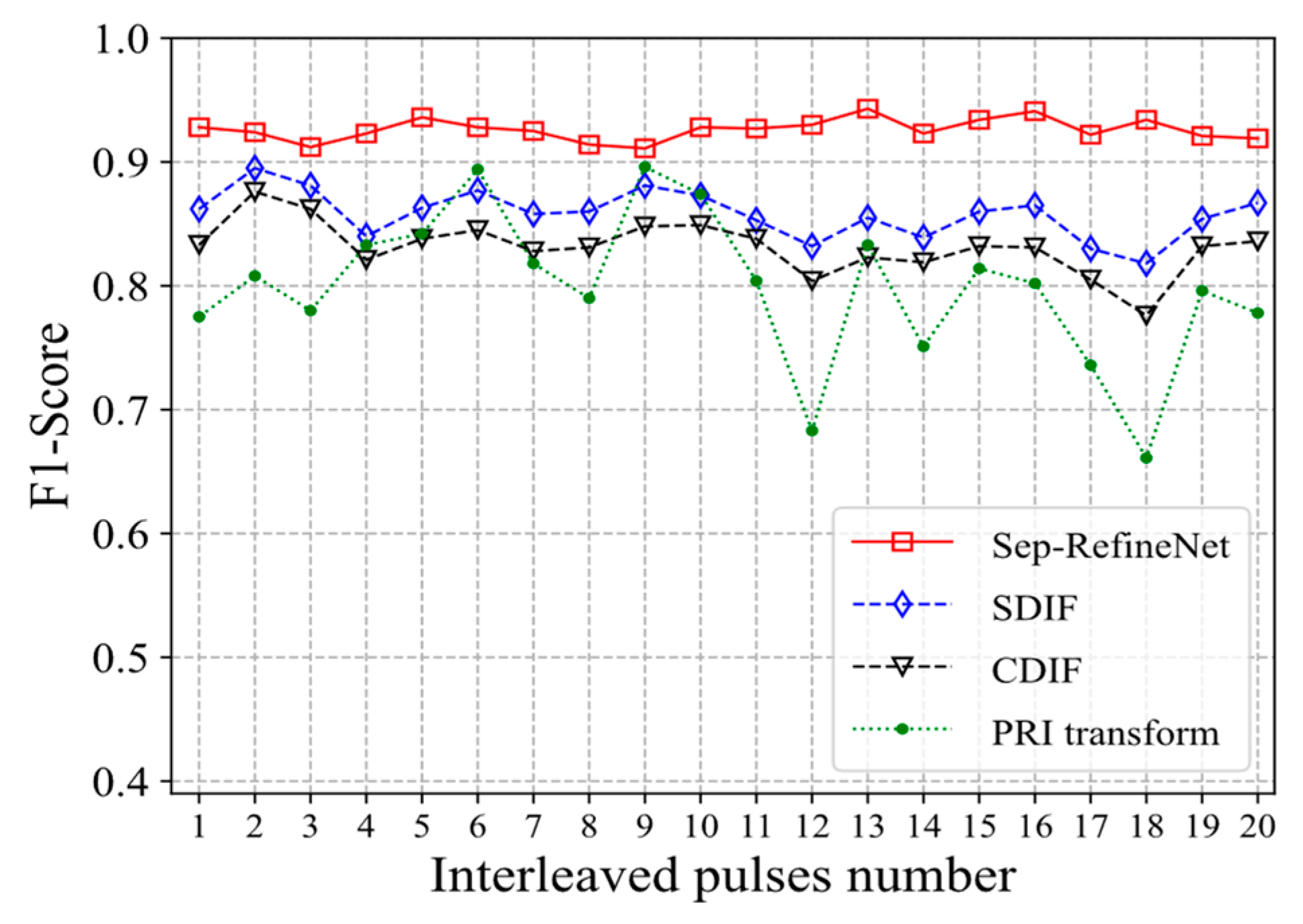
| Aliasing and Missing Rate | 5% | 10% | 15% | 20% |
|---|---|---|---|---|
| F1-Score | ||||
| SDIF | 0.894 | 0.878 | 0.841 | 0.782 |
| CDIF | 0.875 | 0.860 | 0.836 | 0.774 |
| PRI transform | 0.836 | 0.814 | 0.753 | 0.683 |
| Sep-RefineNet | 0.946 | 0.931 | 0.918 | 0.904 |
Disclaimer/Publisher’s Note: The statements, opinions and data contained in all publications are solely those of the individual author(s) and contributor(s) and not of MDPI and/or the editor(s). MDPI and/or the editor(s) disclaim responsibility for any injury to people or property resulting from any ideas, methods, instructions or products referred to in the content. |
© 2023 by the authors. Licensee MDPI, Basel, Switzerland. This article is an open access article distributed under the terms and conditions of the Creative Commons Attribution (CC BY) license (https://creativecommons.org/licenses/by/4.0/).
Share and Cite
Mao, Y.; Ren, W.; Li, X.; Yang, Z.; Cao, W. Sep-RefineNet: A Deinterleaving Method for Radar Signals Based on Semantic Segmentation. Appl. Sci. 2023, 13, 2726. https://doi.org/10.3390/app13042726
Mao Y, Ren W, Li X, Yang Z, Cao W. Sep-RefineNet: A Deinterleaving Method for Radar Signals Based on Semantic Segmentation. Applied Sciences. 2023; 13(4):2726. https://doi.org/10.3390/app13042726
Chicago/Turabian StyleMao, Yongjiang, Wenjuan Ren, Xipeng Li, Zhanpeng Yang, and Wei Cao. 2023. "Sep-RefineNet: A Deinterleaving Method for Radar Signals Based on Semantic Segmentation" Applied Sciences 13, no. 4: 2726. https://doi.org/10.3390/app13042726