
Image Interpolation Based on Spiking Neural Network Model

Department of Computer Technologies, Alanya Alaaddin Keykubat University, 07450 Antalya, Turkey
Appl. Sci. 2023, 13(4), 2438; https://doi.org/10.3390/app13042438
Submission received: 19 December 2022
/
Revised: 11 February 2023
/
Accepted: 13 February 2023
/
Published: 14 February 2023
(This article belongs to the Special Issue Advances in Digital Image Processing)
Abstract
:Image interpolation is used in many areas of image processing. It is seen that many techniques developed to date have been successful in both protecting edges and increasing image quality. However, these techniques generally detect edges with gradient-based linear calculations. In this study, spiking neural networks (SNNs), which are known to successfully simulate the human visual system (HVS), are used to detect edge pixels instead of the gradient. With the help of the proposed SNN-based model, the pixels marked as edges are interpolated with a 1D directional filter. For the remaining pixels, the standard bicubic interpolation technique is used. Additionally, the success of the proposed method is compared to known methods using various metrics. The experimental results show that the proposed method is more successful than the other methods.
1. Introduction
Image interpolation is still used today to improve image quality in many fields of image processing (such as medical sciences, natural sciences, or satellite images), and new techniques continue to be developed [1,2,3]. Generally, interpolation techniques are examined in two groups: super-resolution techniques [4,5,6,7] and sample-free techniques [8,9,10,11,12,13,14]. Super-resolution-based approaches require a training phase based on learning the relationships between low- and high-resolution samples of many images. On the other hand, sample-free methods perform the interpolation process through mathematical formulae without any training steps. Therefore, their most important advantage is that they are fast. The most known sample-free approaches are the nearest, bilinear, and bicubic interpolation methods [15]. Although the most successful results are generally obtained with bicubic interpolation, the most significant disadvantage of this method is edge loss [16].
Recently, many interpolation techniques based on the detection of edge pixels have been developed [8,9,10,11,12,13,14]. The general purpose of these studies is to reduce edge loss and increase image quality by performing different interpolation operations on edge pixels and non-edge pixels. The CGI method [9], proposed in 2013, is one of the first and most well-known techniques to detect edge and non-edge pixels in the interpolation process. The CGI method performs interpolation using a 1D cubic filter for edge pixels and a 2D bicubic filter for non-edge pixels. In 2016, with the development of the CGI method, the CED [10] interpolation technique was proposed. The CED technique also uses different filters according to the edge status of the pixels. A similar approach, the PCI [11] interpolation technique, uses the Canny edge detector in the edge detection phase. The IEDI [8] technique applies different interpolation approaches on the edge and non-edge pixels with the help of the Canny edge detector. On the other hand, the WTCGI [12] technique includes very similar steps to the CGI technique and uses wavelet transform for edge detection. In one of the latest studies, the GEI [14] technique uses gradient-based edge detection, marks the pixels as edge and non-edge, and then applies different interpolation approaches to these pixels.
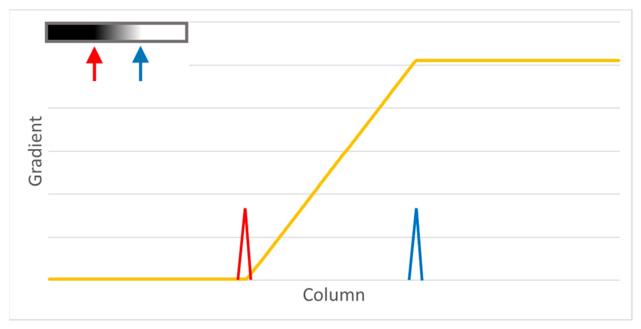
The common feature of edge-based interpolation studies in the literature is that they have used edge detection approaches, such as gradients or wavelets, in which the gray-level differences of neighboring pixels are calculated. Gradient approaches, which are based on the linear difference between the gray-level values of the pixels, have been used for many years for edge detection in many different areas due to their easy calculations [17,18]. The gradient is usually calculated with the help of small-size filters (e.g., 2 × 2 or 3 × 3) [15]. Moreover, the most important disadvantage of the gradient is that it has high noise sensitivity and detects false edges [19]. However, the way the human visual system (HVS) detects edges is quite different from the way gradient-based techniques detect edges. The detection of the gray-level change between pixels of a ganglion cell in HVS [20] is shown in Figure 1. Even if the change in the gradient value is linear, the ganglion cells detect the change at only two points. Therefore, it is clear that different approaches should be used instead of gradients to develop an interpolation technique compatible with HVS.
Especially in the last decade, edge detection techniques inspired by HVS have achieved significant success. In the 2000s, bioinspired edge detection techniques that simulate HVS have begun to be developed as an alternative to gradient-based linear edge detection techniques. In one of the first image processing studies on HVS, a double-layer network design for edge detection was developed in 1993 [21]. It is seen that this double-layer network structure has been used in almost all HVS-based studies carried out to date. In 1998, an approach to pattern analysis that calculates synaptic potentials in a network of neurons was developed [22]. An approach based on the leaky integrate-and-fire (LIF) neuron model for the segmentation of gray-level images was presented in 2005 [23]. It has been observed that SNNs, which process information with the help of spikes generated by connected neurons, are quite successful in HVS-based image processing [24]. For edge detection, the first SNN-based approach was proposed by Wu et al. [25]. The researchers developed a network model in which the gray-level values of pixels are transmitted to neurons in the intermediate layer with the help of excitatory and inhibitory synaptic connections from the receptor layer. The spikes generated in the neurons in the intermediate layer are transmitted to the corresponding neuron in the output layer by excitatory synaptic connections. Similar to the network model in the approach of Wu et al., different receptor and intermediate layers with different matrices and window sizes have been used in many studies [26,27,28,29,30,31,32]. In 2017 [33], an SNN model for edge detection was designed using the Hodgkin and Huxley (HH) [34] neuron model. The HH model, which is much more complex and has a high computational cost was also used by Vemuru [35] for edge detection in 2020. However, in Vemuru’s study, the values of some parameters in the HH neuron model were assumed as 0 and it was seen that the conductance-based integrate and fire (CIF) neuron model was used. An SNN design based on the CIF neuron model for edge detection was also used to calculate the diffusion function of the anisotropic diffusion filter (ADF) in 2022 [36].
Spiking neural network (SNN)-based approaches developed to simulate HVS detect edges more successfully than gradient-based techniques [25,33,35]. The most important reason for this success is that SNN-based approaches detect edges in the image by modeling neurons in HVS instead of linear differences between the gray-level values of the pixels. Additionally, thanks to models and analytical solutions that have been developed, calculations with SNNs can be performed very quickly [35,36].
This study mainly focuses on increasing image interpolation success. Therefore, to increase the success of interpolation, a new SNN-based edge detection approach is proposed instead of gradient, which is highly sensitive to noise. Additionally, a new SNN model is developed for edge detection. Edge detection approaches based on conductance-based integrate and fire neuron models generally use 5 × 5 receptor fields [25,28,35]. Furthermore, the use of the HH neuron model increases the computational cost considerably [33]. It is seen that the edge directions can also be determined as different angles (30 and 60 degrees) [26,27,29,33]. Apart from these, additional filters such as the Gabor filter are also used in the model [35]. The proposed SNN model reduces the computational cost by using 3 × 3 neighborhoods. It also does not include additional filters or additional parameters of the HH model. For these reasons, a new model, which is faster and simpler than other existing SNN models, is proposed. Moreover, instead of calculating the differences between the center pixel and each of its neighbors individually in the 3 × 3 receptor area [36], the proposed model tries to identify edges in 4 different directions.
The success of the proposed method is tested by using the 12 images that are most frequently used in interpolation studies. After the edge detection process with the proposed SNN model, all pixels are first divided into two groups as edge and non-edge pixels. For pixels detected as edges, the 1D interpolation method is used according to the directions of the edges, whereas the bicubic interpolation technique, which is one of the most known methods, is used for non-edge pixels. The proposed method is compared to various edge-based interpolation techniques. The results that are obtained show that the proposed approach is quite successful. Another important aspect of the study is that SNNs are introduced to interpolation for the first time.
The rest of this paper is organized as follows: Chapter 2 introduces the basis of image interpolation. In Chapter 3, the conductance-based integrate-and-fire (CIF) neuron model is described. The proposed SNN model and its integration with the interpolation approach are presented in Chapter 4. Chapter 5 includes the interpolation results of the proposed SNN-based edge detection method and performance comparisons.
2. Image Interpolation
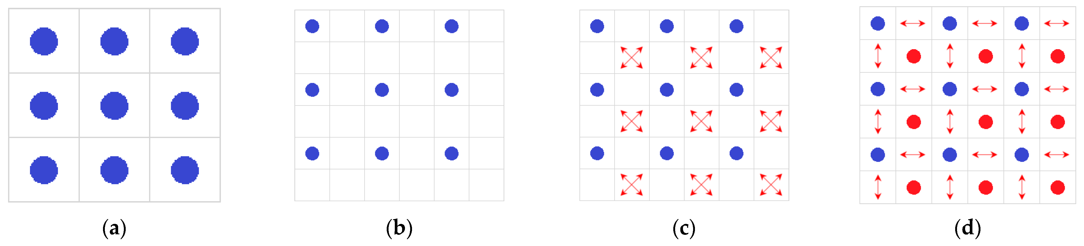
Image interpolation can be expressed as the calculation of unknown pixels with the help of the known pixels. When the M × N-sized IL (low resolution) image is interpolated to the 2 × 2 size as in Figure 2a, a 2M × 2N-sized IH (high resolution) image will be obtained. While creating the IH image, the image in Figure 2b is first created by the process shown in Equation (1).
In general, in edge-based techniques [12,14], after detecting the edges and their directions, the values of the pixels located in the IH(2i, 2j) position indicated by the diagonal arrows in Figure 2c are calculated first. This calculation generally depends on whether the IL(i, j) pixel is an edge pixel with a diagonal angle. The value of the IH(2i, 2j) pixel (if IL(i, j) is an edge pixel with a diagonal angle) is calculated with the help of the known blue-colored pixels adjacent to it. After calculating the diagonally angled pixels, in the second step, calculations are performed for the pixels indicated by the horizontal and vertical arrows in Figure 2d. If a pixel is in the position IH(2i, 2j + 1) and IL(i, j) has a horizontally oriented edge, this pixel is assigned a value using its neighbors on the horizontal plane. Similarly, if a pixel is at the position IH(2i + 1, 2j) and IL(i, j) has a vertically oriented edge, the value of the pixel IH(2i + 1, 2j) is calculated using its neighbors on the vertical plane. Finally, pixels that are not marked as edges are generally assigned using bicubic interpolation. Thus, the values of all pixels in the IH image are determined.
In almost all interpolation studies examined, it is seen that the interpolation process has been carried out to increase the image to a 2 × 2 size. In these studies, experimental results have been obtained by comparing Iorg (original image) to the IH image constructed by first downsampling the Iorg by ½ × ½ and then upsampling it to a 2 × 2 size again. To compare the success of the proposed method in this study, the images used in recent studies are first made 1/2 × 1/2 by downsampling. Although the nearest, bilinear, and bicubic techniques can be used for downsampling, in this study, the direct extraction method is used because it is known to both preserve the original pixels of the image and increase success [14]. When shrinking an image by direct extraction, double-index rows and double-index columns in the image are deleted. Thus, the M × N-sized IL image is obtained directly from the 2M × 2N-sized Iorg image. Then, the methods to be tested are applied to the IL image, and an IH image of a 2M × 2N size is obtained. Finally, the success of the tested method is measured by comparing the Iorg and IH images.
3. Conductance-Based Integrate-and-Fire Neuron Model
In 1952, Hodgkin and Huxley [34] introduced a model for simulating actions in neurons with the help of differential equations. However, the HH neuron model has a high computational cost since it has many differential equations and parameters. Therefore, different neuron models such as integrate-and-fire (IF), FitzHugh–Nagumo (FHN), and Izhikevich have been presented [37,38,39]. Among these models, the CIF neuron model [40] stands out with its lower computational cost advantage in large-scale networks [41]. In the CIF model, the membrane potential is calculated by Equation (2).
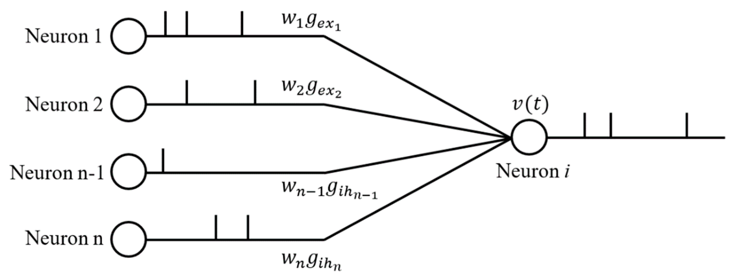
where cm is the membrane capacitance. gl is the membrane conductance and El is the reverse potential of the membrane. Eex and Eih are the reverse potentials of excitatory and inhibitory synapses, respectively. wex and wih are the weights of the synapses, and Aex and Aih are the membrane surface areas. gex and gih represent the time-varying conductance of excitatory and inhibitory synapses. If a neuron’s excitatory connections send a higher signal than its inhibitory connections, the neuron’s membrane potential exceeds the threshold voltage 𝑣th at time t, and the neuron generates a spike. Immediately after this, from the moment t + 1, the membrane potential of the neuron remains constant at its initial value 𝑣reset for a time τref, called the refractory time. For the simplicity of the model and ease of calculation, the τref value was accepted as 0 in this study as in similar studies [27,31,32]. Figure 3 illustrates the spike sequence produced by a neuron (Neuron i) according to signals from synaptically connected neurons.
4. Proposed Method
In this section, the SNN model proposed for image interpolation using edge detection is explained. Then, the image interpolation process is given in detail.
4.1. Proposed SNN Model for Edge Detection
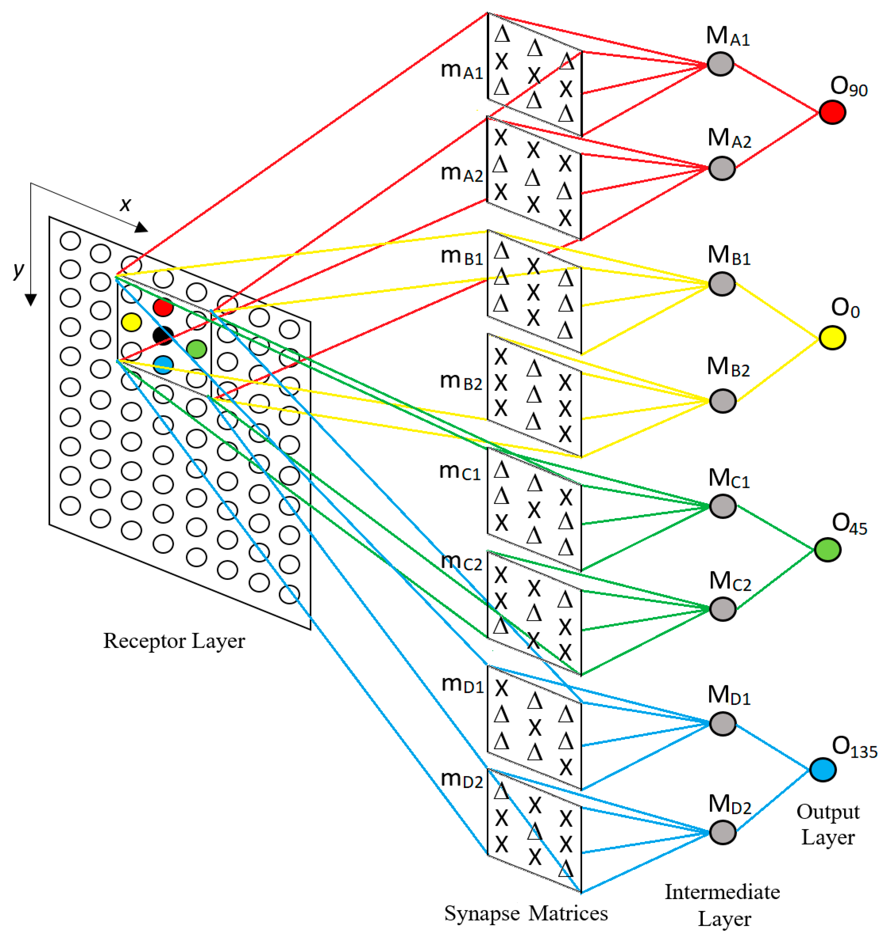
In this study, a new SNN model shown in Figure 4 is proposed for edge detection to be used in the interpolation process. The proposed model consists of three layers. The first layer is the receptor layer, which transmits the gray-level values from the pixels to the neurons. The network model detects the edges in four different directions (0°, 45°, 90°, and 135°) for an image. Although the structure of the proposed SNN model is based on the model developed for ADFs [36], the interlayer structure is modified for line detection [29] purposes to detect edges. Thus, the edges in four different directions are obtained as four different output values instead of a single output value.
In the first layer, the receptor layer, each pixel in the SNN model corresponds to a receptor. Data from the receptor layer are transmitted to the intermediate layer via synaptic connections. Each of all eight neurons in the intermediate layer is connected to the receptor layer by different synaptic connections. The connections of the neurons in the intermediate layer are structured with the help of synaptic matrices. X and ∆ symbols in synaptic matrices indicate excitatory and inhibitory synapses, respectively. The neurons in the intermediate layer are connected to four separate output neurons in pairs according to their edge directions. The firing number of each neuron in the output layer in a time interval corresponds to the gray-level value of the edge image specified by the output neuron. Thus, each output neuron creates a gray-level edge image.
In the receptor layer, there is a 3 × 3 receptor field (RF) that centers each pixel in the image. Each RF is connected to eight neurons in the intermediate layer (MA1, MA2, MB1, MB2, MC1, MC2, MD1, and MD2) with eight individual synaptic matrices (mA1, mA2, mB1, mB2, mC1, mC2, mD1, and mD2). Each pair of neurons in the intermediate layer determines the edges located at the angles 90°, 0°, 45°, and 135°, respectively. For example, synaptic signals from RF to MA1 via mA1 are calculated between the horizontal pixels in the center and the other six neighboring pixels. The center pixel in the RF and its neighbors to its left and right have an excitatory synaptic connection through the matrix mA1, whereas other pixels have an inhibitory synaptic connection. If the excitatory pixels have a higher gray-level value than the inhibitory pixels, the membrane potential of the neuron MA1 will increase and the neuron will generate spikes at intervals. Otherwise, the membrane potential of mA1 will not change and the neuron will not generate any spike. The same is true for the neuron MA2, which has synaptic connections opposite to that of the neuron MA1. In the matrix mA2, the central pixel and its left and right neighbors have inhibitory synaptic connections, whereas the other six neighbors have excitatory connections. So, if the pixels on the central horizontal plane have a lower gray-level value than those of the other neighbors, the membrane potential of the neuron MA2 will increase and the neuron will generate spike(s). The greater the difference between the signals from the excitatory and inhibitory synapses, the higher the frequency of spike generation will be. If the pixels on the central horizontal plane and the gray-level values of the other six neighbors are the same or close, neither of the neurons MA1 and MA2 will generate spikes.
It is known that HVS does not linearly calculate the difference between the gray-level values of pixels like the gradient, but it determines this difference according to the firing levels of neurons with inhibitory and excitatory synaptic connections [42]. Therefore, it is aimed at detecting the edge directions in a 3 × 3 neighborhood by using two different synaptic matrices for each edge direction in this study.
If the neurons MA1 or MN2 generate spikes at certain intervals, these generated spikes will be transmitted to neuron O90 in the output layer. In the proposed model, the pairs of neurons in the intermediate layer have only excitatory synaptic connections with the corresponding neuron in the output layer. Depending on the intensity of the synaptic signals from MA1 and MA2, the output neuron O90 will also generate spikes at certain intervals. A similar situation is realized in other output neurons (O0, O45, and O135), and edge images are obtained at four different angles.
The CIF neuron model used for visual attention [29] is applied to the proposed SNN in this study. (x, y) in the SNN represents the coordinates of the pixels corresponding to the receivers. The peak conductivity values qex and qih of excitatory and inhibitory receptors are calculated by Equation (3). Gx,y is the gray-level value of the pixel at the (x, y) coordinate.
where α and β are the coefficients used to normalize the gray-level values between 0 and 1 and are accepted as 1/255. For clarity, only the equations for the MA1 neuron are given below. Calculations for each neuron in the intermediate layer are performed with the same equations.
where τex and τih are the time constants for excitatory and inhibitory synapses, respectively.
where Isyn is the total synaptic current from the synaptic connections. Equation (7) which is the analytical solution to Equation (2), is used to calculate the membrane potential v(t) of the MA1 neuron [35].
In the matrix mA1, which determines the synaptic connections of the neuron MN1, gex is the total conductivity of the receptor of the central pixel and receptors of its left and right neighbors. gih, on the other hand, refers to the conductivity of the receptors of the six pixels located on the top and bottom rows of the central pixel. For the neuron MA2, the connections to the receptors of the same pixels are expressed as in the matrix mN2. In mN2, the center pixel and its left and right neighbors have inhibitory connections and the other neighbors have excitatory connections.
Calculations for MA1 are also performed for neurons MA2, MB1, MB2, MC1, MC2, MD1, and MD2. If the membrane potential of a neuron in the network achieves its threshold value, the neuron generates spike(s). The generated spikes are stored in a separate spike train for each neuron. SA1, the spike sequence of the MA1 neuron, is determined by Equation (8).
The four output neurons in the output layer have only excitatory synaptic connections with pairs of neurons in the intermediate layer. Calculations for output neurons are performed by Equations (9)–(11).
where gout is the conductivity value, τout is the time constant, Iout is the total synaptic current, Eout is the reverse potential for synapses, and v(t)O90 is the membrane potential of the O90 neuron. SA1 and SA2 are the spike trains of the MA1 and MA2 neurons, respectively. The spike train O90 of the neuron S90 is also calculated by Equation (8). The number of spikes F90 generated by the output neuron O90 during time T can be calculated by Equation (12). The spike numbers of other output neurons are also calculated using the equations above.
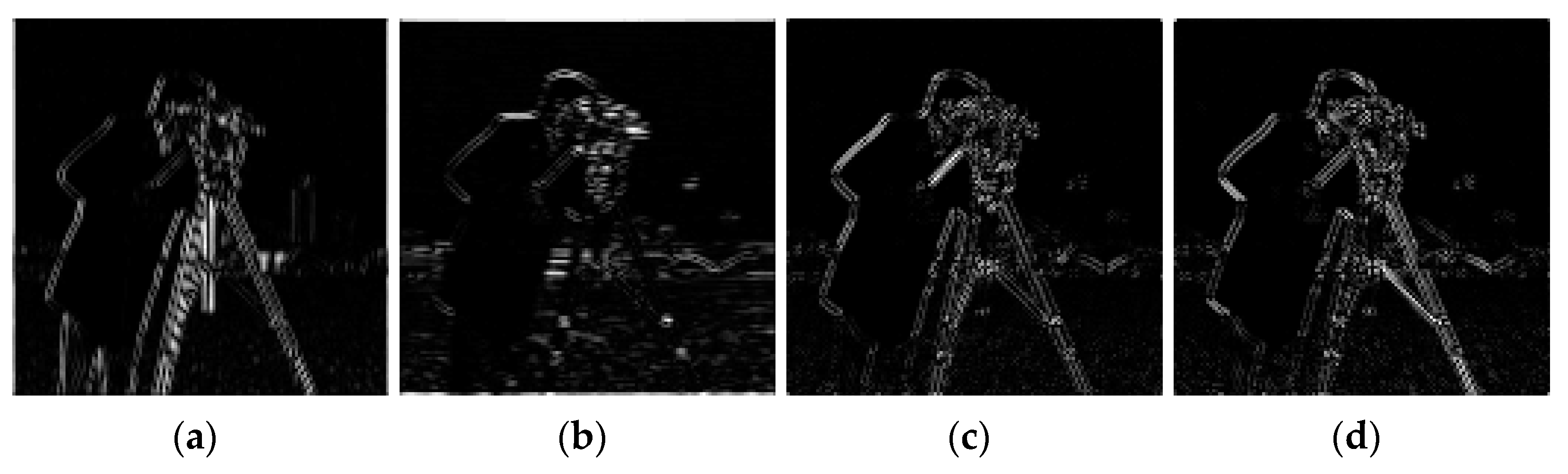
Instead of edges obtained using gradient-based edge detection approaches, edge images consisting of F values, which include the number of spikes produced by each output neuron during time T, are determined by HVS with the help of SNNs. The edge images of the proposed model are given in Figure 5.
Whereas vertical lines are more prominent in Figure 5a, horizontal lines are seen uninterrupted and distinctly in Figure 5b. The edges at angles 45° and 135° appear uninterrupted and distinctly in Figure 5c,d. The edge information from the four angles obtained with the proposed SNN model is used when calculating the image interpolation.
4.2. Image Interpolation with SNN-Based Edge Detection
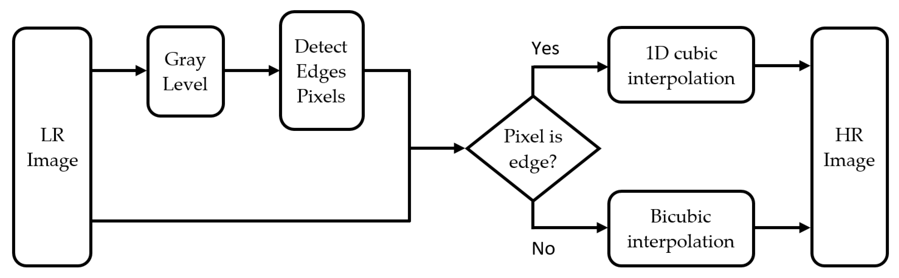
The method used for image interpolation in this study includes the steps shown in Figure 6. In general, these steps have been frequently included in recent studies in the field of interpolation in the literature. The most important difference of the proposed method is that it determines the edges and edge directions with an SNN model. In the first step, gray-level conversion is performed for IL. Then, the edges of the gray-level image in four different directions are determined by the proposed SNN model. Afterward, whether the pixel is an edge pixel or a non-edge pixel is checked. If the pixel is marked as an edge pixel, its direction is determined.
While checking the edge or non-edge status of the pixel, it is needed to first examine whether it is included in one of the diagonal or linear edges.
If there is no difference between the values of F45(i, j) and F135(i, j), which are the SNN outputs of the gray-level transform of the IL image in Equation (13), the pixel in IH(2i, 2j) is considered a non-edge pixel and no assignment is performed. If F45(i, j) is greater than F135(i, j), θ(2i, 2j) is assigned 45°, whereas otherwise, it is assigned 135°. The same procedure is then performed for the pixels IH(2i−1, 2j) and IH(2i, 2j−1) whose known neighbors are horizontal and vertical.
In Equation (14), if F90(i, j) and F0(i, j), which are the SNN outputs of the gray-level transform of the IL image, are equal to each other, then, IH(2i − 1, 2j) and IH(2i, 2j − 1) are defined as non-edge pixels. If F90(i, j) is greater than F0(i, j), θ(2i − 1, 2j) and θ(2i, 2j − 1) are assigned 90°, they are assigned 0° otherwise.
After the edge directions are detected, firstly, the pixels at IL(i, j) are transferred to IH(2i − 1, 2j − 1) as shown in Figure 2b. Then, the same operations are applied to the pixels in Figure 2c,d, respectively. Thus, all the pixels marked as edges are interpolated. If the pixels IH(2i, 2j), IH(2i, 2j − 1), and IH(2i − 1, 2j) are marked as edges, their values are calculated using Equations (15)–(19), which have also been used in different studies [12,14].
where w is an interpolation coefficient, and its value is 0.575 [12,14]. Let us assume that the indices of the 2M × 2N-sized IH image are p and q. If θ(p, q) has an angle of 45°:
If θ(p, q) = 135°:
If θ(p, q) = 0°:
If θ(p, q) = 90°:
Finally, bicubic interpolation is applied for the IH(2i, 2j), IH(2i, 2j − 1), and IH(2i − 1, 2j) pixels, which are marked as non-edge, and an IH image is obtained. In this study, the interpolation process refers to 2 × 2 upsampling.
5. Experimental Results
The proposed method is tested on the 12 most commonly used images for testing interpolation techniques. The results are obtained with the CGI [9], CED [10], PCI [11], and IEDI [8] techniques for all images. Apart from these, the results of the recently developed WTCGI [12] and GEI [14] techniques are also included in the comparisons. First, all images are originally downsampled to a size of ½×½. Then, by upsampling to 2 × 2 with the tested methods, the obtained images are ensured to be the same size as the original image. The upsampled images are compared to the original images, and the results are obtained as PSNR and SSIM.
The proposed SNN model is tested in MATLAB with the following parameters: cm = 1 μF/mm2, El = −44.42 mV, gl = 0.003 μS/mm2, τex = 4 ms, τih = 10 ms, τref = 0 ms, Eex = 36.78 mV, Eih = −72.14 mV, Eout = 36.78 mV, vreset = −70 mV, 𝑣th = −55 mV, Aex = 0.0141 mm2, Aih = 0.0281 mm2, T = 100 ms, and dt = 0.1 ms. The weight matrices of the synapses for mA1 and mA2 are as follows:
Table 1 shows the PSNR results of the techniques that are compared in this study. The best results are marked in bold. According to the PSNR results, the proposed method is more successful both in individual images and on average. When compared with the relatively new and successful PCI and GEI techniques, it is seen that using the edges detected by the proposed SNN model increases the success of interpolation.
Another metric used to evaluate the performance of the proposed method is SSIM. According to the SSIM results in Table 2, the proposed method is more successful than the other techniques under investigation. The proposed method has significant success versus both PCI and GEI techniques for each of the 12 images tested in terms of SSIM metric. The success of the proposed method according to the SSIM metric [43], which is known to correlate well with human visual perception, is another indicator of the usefulness of SNN-based approaches modeling HVS.
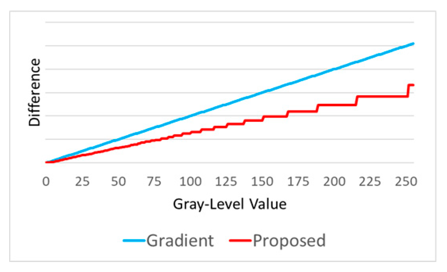
The most important difference that distinguishes the proposed method from state-of-the-art techniques is that the edge pixels are determined with a new SNN model that simulates HVS instead of gradient-based techniques. The clearest advantage of SNNs is the detection of edge angles without a threshold value. The general condition for a pixel to be defined as an edge is |F0(i, j) − F90(i, j)| ≥ T in the WTCGI and GEI techniques. T is a user-defined threshold value. The T value, which is generally used as a constant, is accepted as 0.01 in GEI. As seen in Figure 7, the edge values obtained with SNNs change as non-linear values, as opposed to linear ones as in a gradient. Thus, there is no need to select a threshold value.
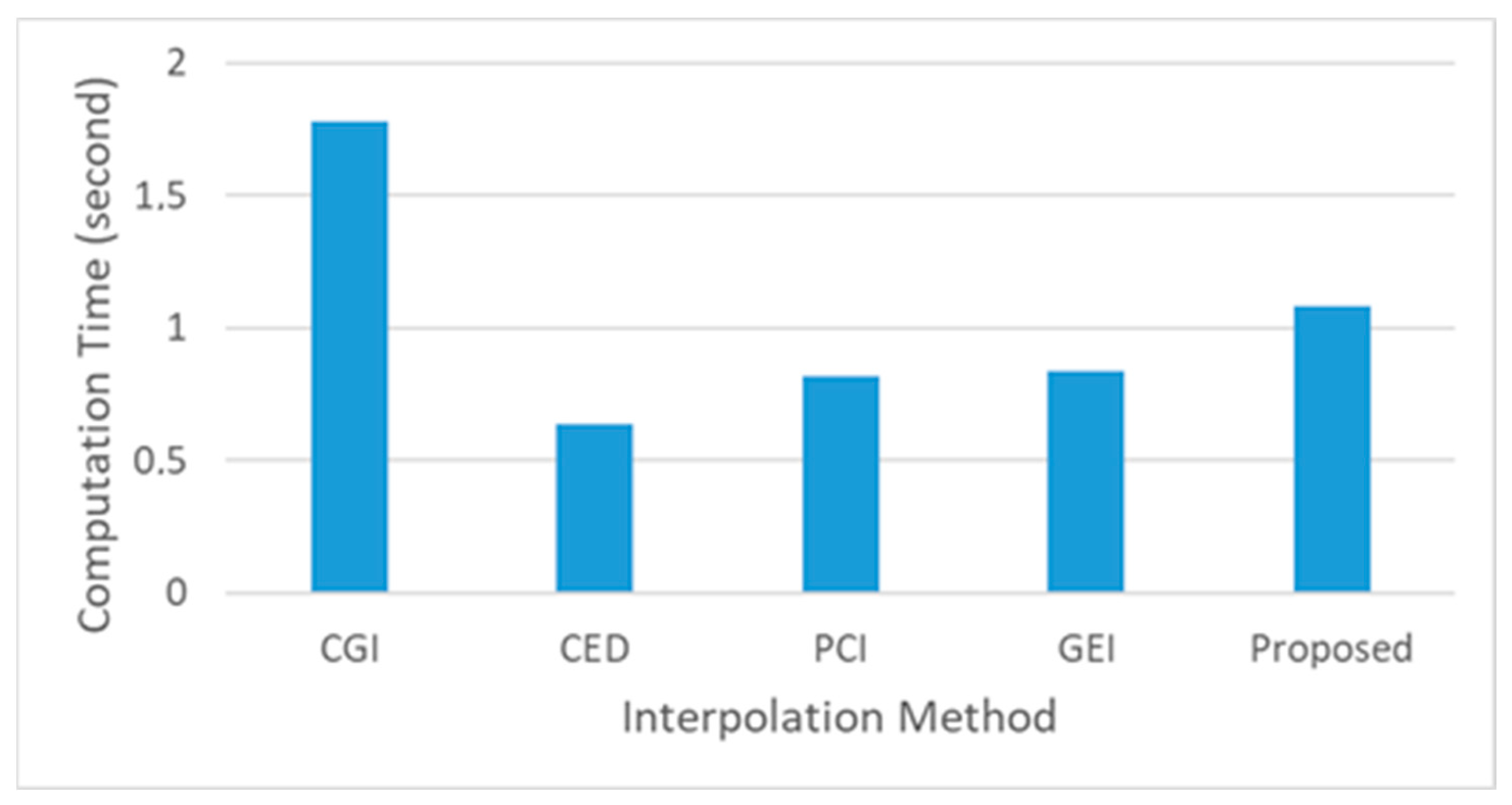
When the interpolation results seen in Figure 8 are examined visually, it is seen that the edges are preserved in a similar way to other techniques in the literature. Although the proposed method produces successful results, the computational time of the SNN model is slightly longer than those of gradient-based techniques. However, the tests show that this difference is tolerable. Figure 9 shows the average calculation times for the results obtained through MATLAB. The tests are run on a computer with an Intel Core i7 4710HQ 2.50 GHz processor and 32GB RAM. Although the proposed method is somewhat behind in terms of calculation times, it can be easily argued that this difference is minimal. This is quite inspiring for studies that can perform edge detection by HVS.
The proposed SNN model is designed in a simpler way than existing SNN models. First of all, since the receptor field utilized is 3 × 3 in size, the computational cost of the proposed method is approximately 1/2.5 times those in studies using 5 × 5 dimension receptor fields [25,28,35]. Additionally, it does not contain additional filters such as the Gabor filter which also provides an advantage in terms of the computational cost. Another important aspect of the proposed approach is that it does not require any learning steps while detecting edges, just like gradient-based techniques. The proposed approach provides successful results by simulating HVS in a much simpler way compared to known machine learning (ML) techniques. The results obtained in this study, where SNNs are used for the first time for interpolation, will open the door to many similar studies in the future.
6. Conclusions
In recent years, many techniques in which the edges of an image are used to increase the success of interpolation have been developed. However, current techniques use approaches such as gradients or wavelets that calculate the gray-level difference between pixels linearly. Additionally, it is observed that previously developed techniques include very similar steps, and the greatest differences are in the edge detection processes. On the other hand, it is known that the edge detection success of SNNs simulating the HVS is quite high. In this study, a new SNN model is proposed to be used in the interpolation process. Whereas 1D cubic interpolation is applied on the edge pixels determined using the proposed SNN model, standard bicubic interpolation is applied to the others. The success of the proposed method is compared to other edge-based interpolation methods using the PSNR and SSIM metrics. The results that are obtained show that the SNN-based method, which is used for the first time in interpolation studies, is quite successful. Additionally, the fact that the running time of the proposed method is not very long compared to other methods shows that it can be used in different image processing studies where the detection of edge directions is important. In the future, the proposed SNN model is planned to be used in other image-processing fields based on edge detection.
Funding
This research received no external funding.
Institutional Review Board Statement
Not applicable.
Informed Consent Statement
The study did not involve humans.
Data Availability Statement
Data sharing is not applicable.
Conflicts of Interest
The author declares no conflict of interest.
References
- Pramunendar, R.A.; Wibirama, S.; Santosa, P.I. Fish Classification Based on Underwater Image Interpolation and Back-propagation Neural Network. In Proceedings of the 2019 5th International Conference on Science and Technology, ICST 2019, Yogyakarta, Indonesia, 30–31 July 2019. [Google Scholar]
- Moraes, T.; Amorim, P.; Da Silva, J.V.; Pedrini, H. Medical Image Interpolation Based on 3D Lanczos Filtering. Comput. Methods Biomech. Biomed. Eng. Imaging Vis. 2020, 8, 294–300. [Google Scholar] [CrossRef]
- Cardona, J.G.; Ortega, A.; Rodriguez-Alvarez, N. Graph-Based Interpolation for Remote Sensing Data. In Proceedings of the 2022 30th European Signal Processing Conference (EUSIPCO), Belgrade, Serbia, 29 August–2 September 2022; pp. 1791–1795. [Google Scholar]
- Saharia, C.; Ho, J.; Chan, W.; Salimans, T.; Fleet, D.J.; Norouzi, M. Image Super-Resolution via Iterative Refinement. IEEE Trans. Pattern Anal. Mach. Intell. 2022, 1–14. [Google Scholar] [CrossRef] [PubMed]
- Lugmayr, A.; Danelljan, M.; Van Gool, L.; Timofte, R. SRFlow: Learning the Super-Resolution Space with Normalizing Flow. In Lecture Notes in Computer Science (Including Subseries Lecture Notes in Artificial Intelligence and Lecture Notes in Bioinformatics); Springer Science + Business Media: Berlin, Germany, 2020; Volume 12350. [Google Scholar]
- Mei, Y.; Fan, Y.; Zhou, Y. Image Super-Resolution with Non-Local Sparse Attention. In Proceedings of the IEEE Computer Society Conference on Computer Vision and Pattern Recognition, Virtual, 19–25 June 2021. [Google Scholar]
- Wang, P.; Bayram, B.; Sertel, E. A Comprehensive Review on Deep Learning Based Remote Sensing Image Super-Resolution Methods. Earth-Sci. Rev. 2022, 232, 104110. [Google Scholar] [CrossRef]
- Hossain, M.S.; Jalab, H.A.; Kahtan, H.; Abdullah, A. Image Resolution Enhancement Using Improved Edge Directed Interpolation Algorithm. In Proceedings of the 9th IEEE International Conference on Control System, Computing and Engineering, ICCSCE 2019, Penang, Malaysia, 29 November–1 December 2019. [Google Scholar]
- Wei, Z.; Ma, K.K. Contrast-Guided Image Interpolation. IEEE Trans. Image Process. 2013, 22, 4271–4285. [Google Scholar] [CrossRef] [PubMed]
- Ye, W.; Ma, K.K. Convolutional Edge Diffusion for Fast Contrast-Guided Image Interpolation. IEEE Signal Process. Lett. 2016, 23, 1260–1264. [Google Scholar] [CrossRef]
- Zhong, B.; Ma, K.K.; Lu, Z. Predictor-Corrector Image Interpolation. J. Vis. Commun. Image Represent. 2019, 61, 50–60. [Google Scholar] [CrossRef]
- Zhao, Y.; Huang, Q. Image Enhancement of Robot Welding Seam Based on Wavelet Transform and Contrast Guidance. Int. J. Innov. Comput. Inf. Control 2022, 18, 149–159. [Google Scholar] [CrossRef]
- Lama, R.K.; Shin, S.; Kang, M.; Kwon, G.R.; Choi, M.R. Interpolation Using Wavelet Transform and Discrete Cosine Transform for High Resolution Display. In Proceedings of the 2016 IEEE International Conference on Consumer Electronics, ICCE 2016, Las Vegas, NV, USA, 7–11 January 2016. [Google Scholar]
- Jia, Z.; Huang, Q. Image Interpolation with Regional Gradient Estimation. Appl. Sci. 2022, 12, 7359. [Google Scholar] [CrossRef]
- Pratt, W.K. Digital Image Processing, 4th Edition. J. Electron. Imaging 2007, 16, 029901. [Google Scholar] [CrossRef]
- Singh, A.; Singh, J. Review and Comparative Analysis of Various Image Interpolation Techniques. In Proceedings of the 2019 2nd International Conference on Intelligent Computing, Instrumentation and Control Technologies, ICICICT 2019, Kannur, India, 5–6 July 2019; pp. 1214–1218. [Google Scholar]
- Palconit, M.G.B.; Conception, R.S.; Alejandrino, J.D.; Evangelista, I.R.S.; Sybingco, E.; Vicerra, R.R.P.; Bandala, A.A.; Dadios, E.P. Counting of Uneaten Floating Feed Pellets in Water Surface Images Using ACF Detector and Sobel Edge Operator. In Proceedings of the IEEE Region 10 Humanitarian Technology Conference, R10-HTC, Bangalore, India, 30 September–2 October 2021; Institute of Electrical and Electronics Engineers Inc.: Piscataway, NJ, USA, 2021. [Google Scholar]
- Wu, F.; Zhu, C.; Xu, J.; Bhatt, M.W.; Sharma, A. Research on Image Text Recognition Based on Canny Edge Detection Algorithm and K-Means Algorithm. Int. J. Syst. Assur. Eng. Manag. 2022, 13, 72–80. [Google Scholar] [CrossRef]
- Chandwadkar, R.; Dhole, S.; Gadewar, V.; Raut, D.; Tiwaskar, P.S.A. Comparison of Edge Detection Techniques. In Proceedings of the Sixth IRAJ International Conference, Pune, India, 6 October 2013; pp. 133–136. [Google Scholar]
- Keil, M.S.; Cristóbal, G.; Neumann, H. Gradient Representation and Perception in the Early Visual System—A Novel Account of Mach Band Formation. Vision Res. 2006, 46, 2659–2674. [Google Scholar] [CrossRef] [PubMed]
- Manjunath, B.S.; Chellappa, R. A Unified Approach to Boundary Perception: Edges, Textures, and Illusory Contours. IEEE Trans. Neural Netw. 1993, 4, 96–108. [Google Scholar] [CrossRef]
- Natschläger, T. Spatial and Temporal Pattern Analysis via Spiking Neurons. Netw. Comput. Neural Syst. 1998, 9, 319–332. [Google Scholar] [CrossRef]
- Buhmann, J.M.; Lange, T.; Ramacher, U. Image Segmentation by Networks of Spiking Neurons. Neural Comput. 2005, 17, 1010–1031. [Google Scholar] [CrossRef]
- Ghosh-Dastidar, S.; Adeli, H. Spiking Neural Networks. Int. J. Neural Syst. 2009, 19, 295–308. [Google Scholar] [CrossRef] [PubMed]
- Wu, Q.X.; McGinnity, M.; Maguire, L.; Belatreche, A.; Glackin, B. Edge Detection Based on Spiking Neural Network Model. In Lecture Notes in Computer Science (Including Subseries Lecture Notes in Artificial Intelligence and Lecture Notes in Bioinformatics); Springer Science + Business Media: Berlin, Germany, 2007; Volume 4682. [Google Scholar]
- Clogenson, M.; Kerr, D.; McGinnity, M.; Coleman, S.; Wu, Q. Biologically Inspired Edge Detection Using Spiking Neural Networks and Hexagonal Images. In Proceedings of the International Conference on Neural Computation Theory and Applications, Paris, France, 24–26 October 2011. [Google Scholar]
- Kerr, D.; Coleman, S.; McGinnity, M.; Wu, Q.X.; Clogenson, M. Biologically Inspired Edge Detection. In Proceedings of the International Conference on Intelligent Systems Design and Applications, ISDA, Cordoba, Spain, 22–24 November 2011. [Google Scholar]
- Kerr, D.; McGinnity, M.; Coleman, S.; Wu, Q.; Clogenson, M. Spiking Hierarchical Neural Network for Corner Detection. In Proceedings of the International Conference on Neural Computation Theory and Applications, Paris, France, 24–26 October 2011; pp. 230–235. [Google Scholar]
- Wu, Q.X.; McGinnity, T.M.; Maguire, L.; Cai, R.; Chen, M. A Visual Attention Model Based on Hierarchical Spiking Neural Networks. Neurocomputing 2013, 116, 3–12. [Google Scholar] [CrossRef]
- Kerr, D.; Coleman, S.; McGinnity, M.T. Biologically Inspired Intensity and Depth Image Edge Extraction. IEEE Trans. Neural Netw. Learn. Syst. 2018, 29, 5356–5365. [Google Scholar] [CrossRef] [PubMed]
- Kerr, D.; Coleman, S.A.; McGinnity, T.M.; Clogenson, M. Biologically Inspired Intensity and Range Image Feature Extraction. In Proceedings of the International Joint Conference on Neural Networks, Dallas, TX, USA, 4–9 August 2013. [Google Scholar]
- Kerr, D.; McGinnity, T.M.; Coleman, S.; Clogenson, M. A Biologically Inspired Spiking Model of Visual Processing for Image Feature Detection. Neurocomputing 2015, 158, 268–280. [Google Scholar] [CrossRef]
- Yedjour, H.; Meftah, B.; Lézoray, O.; Benyettou, A. Edge Detection Based on Hodgkin–Huxley Neuron Model Simulation. Cogn. Process. 2017, 18, 315–323. [Google Scholar] [CrossRef]
- Hodgkin, A.L.; Huxley, A.F. A Quantitative Description of Membrane Current and Its Application to Conduction and Excitation in Nerve. J. Physiol. 1952, 117, 500–544. [Google Scholar] [CrossRef] [PubMed]
- Vemuru, K.V. Image Edge Detector with Gabor Type Filters Using a Spiking Neural Network of Biologically Inspired Neurons. Algorithms 2020, 13, 165. [Google Scholar] [CrossRef]
- İncetaş, M.O. Anisotropic Diffusion Filter Based on Spiking Neural Network Model. Arab. J. Sci. Eng. 2022, 47, 9849–9860. [Google Scholar] [CrossRef]
- Fitzhugh, R. Mathematical Models of Excitation and Propagation in Nerve. Biol. Eng. 1969, 9, 1–85. [Google Scholar]
- Nagumo, J.; Arimoto, S.; Yoshizawa, S. An Active Pulse Transmission Line Simulating Nerve Axon*. Proc. IRE 1962, 50, 2061–2070. [Google Scholar] [CrossRef]
- Izhikevich, E.M. Simple Model of Spiking Neurons. IEEE Trans. Neural Netw. 2003, 14, 1569–1572. [Google Scholar] [CrossRef] [PubMed]
- Destexhe, A. Conductance-Based Integrate-and-Fire Models. Neural Comput. 1997, 9, 503–514. [Google Scholar] [CrossRef]
- Wu, Q.X.; McGinnity, M.; Maguire, L.; Glackin, B.; Belatreche, A. Learning Mechanisms in Networks of Spiking Neurons. Stud. Comput. Intell. 2006, 35, 171–197. [Google Scholar] [CrossRef]
- Bull, D.R. Communicating Pictures: A Course in Image and Video Coding; Academic Press: Cambridge, MA, USA, 2014; ISBN 9780080993744. [Google Scholar]
- Wang, Z.; Bovik, A.C.; Sheikh, H.R.; Simoncelli, E.P. Image Quality Assessment: From Error Visibility to Structural Similarity. IEEE Trans. Image Process. 2004, 13, 600–612. [Google Scholar] [CrossRef] [Green Version]
Figure 1.
Responses of a retinal ganglion cell.

Figure 2.
Example of edge-based interpolation. (a) 3 × 3 low-resolution image IL; (b) 6 × 6 high-resolution image IH with known pixels of IL; (c) pixels with diagonal neighborhoods in IH; (d) pixels with linear neighborhoods in IH.
Figure 2.
Example of edge-based interpolation. (a) 3 × 3 low-resolution image IL; (b) 6 × 6 high-resolution image IH with known pixels of IL; (c) pixels with diagonal neighborhoods in IH; (d) pixels with linear neighborhoods in IH.

Figure 3.
Example of synaptic connections of conductance-based IF neuron model.

Figure 4.
Proposed SNN model.

Figure 5.
Edge outputs of proposed SNN model for cameraman image IL. (a) F0; (b) F90; (c) F45; (d) F135.
Figure 5.
Edge outputs of proposed SNN model for cameraman image IL. (a) F0; (b) F90; (c) F45; (d) F135.

Figure 6.
Flowchart of the proposed method.

Figure 7.
Calculated difference values between a pixel and its neighbor with 0 (zero) gray level using the gradient and the proposed SNN model.
Figure 7.
Calculated difference values between a pixel and its neighbor with 0 (zero) gray level using the gradient and the proposed SNN model.

Figure 8.
Examples of interpolation results. (a) Original images; (b) GEI interpolation results; (c) the results of the proposed method.
Figure 8.
Examples of interpolation results. (a) Original images; (b) GEI interpolation results; (c) the results of the proposed method.

Figure 9.
Average run-time of interpolation techniques (second).


Table 1.
PSNR comparison results of interpolation techniques.
| Image | CGI | CED | PCI | IEDI | WTCGI | GEI | Proposed |
|---|---|---|---|---|---|---|---|
| Bike | 25.82 | 25.82 | 25.90 | 25.17 | 25.21 | 25.85 | 26.60 |
| Wheel | 21.01 | 20.98 | 21.22 | 20.31 | 20.57 | 21.32 | 21.53 |
| Boats | 29.51 | 29.56 | 29.77 | 29.24 | 29.32 | 29.42 | 29.71 |
| Butterfly | 29.27 | 29.24 | 29.31 | 28.97 | 28.97 | 29.26 | 29.55 |
| House | 32.83 | 32.71 | 32.88 | 32.31 | 31.87 | 32.84 | 33.17 |
| Cameraman | 25.86 | 25.9 | 25.81 | 25.48 | 25.76 | 25.83 | 26.09 |
| Baboon | 22.50 | 22.41 | 22.53 | 22.41 | 22.35 | 22.59 | 22.82 |
| Peppers | 30.88 | 30.77 | 30.87 | 30.47 | 30.19 | 30.81 | 31.12 |
| Fence | 25.70 | 25.63 | 25.84 | 25.61 | 25.69 | 25.75 | 26.01 |
| Airplane | 26.54 | 26.49 | 26.59 | 26.6 | 26.10 | 26.61 | 26.88 |
| Barbara | 23.75 | 23.64 | 23.82 | 23.54 | 23.41 | 24.01 | 24.25 |
| Stars | 34.13 | 33.94 | 34.38 | 33.36 | 33.71 | 34.33 | 34.67 |
| Average | 27.32 | 27.26 | 27.41 | 26.96 | 26.93 | 27.39 | 27.70 |
Table 2.
SSIM comparison results of interpolation techniques.
| Image | CGI | CED | PCI | IEDI | WTCGI | GEI | Proposed |
|---|---|---|---|---|---|---|---|
| Bike | 0.8808 | 0.8812 | 0.8803 | 0.8751 | 0.8791 | 0.8798 | 0.9071 |
| Wheel | 0.8621 | 0.8626 | 0.8668 | 0.8644 | 0.8649 | 0.8665 | 0.8986 |
| Boats | 0.8763 | 0.8801 | 0.8794 | 0.8771 | 0.8744 | 0.8796 | 0.8963 |
| Butterfly | 0.9721 | 0.9732 | 0.9720 | 0.9718 | 0.9698 | 0.9758 | 0.9992 |
| House | 0.8781 | 0.8778 | 0.8789 | 0.8783 | 0.8775 | 0.8780 | 0.8956 |
| Cameraman | 0.8711 | 0.8732 | 0.8715 | 0.8704 | 0.8692 | 0.8732 | 0.8976 |
| Baboon | 0.9125 | 0.9111 | 0.9130 | 0.9121 | 0.9112 | 0.9165 | 0.9403 |
| Peppers | 0.9032 | 0.9041 | 0.9035 | 0.9029 | 0.9026 | 0.9025 | 0.9278 |
| Fence | 0.7752 | 0.7780 | 0.7785 | 0.7763 | 0.7765 | 0.7723 | 0.7893 |
| Airplane | 0.9405 | 0.9410 | 0.9401 | 0.9389 | 0.9422 | 0.9412 | 0.9591 |
| Barbara | 0.9125 | 0.9128 | 0.9130 | 0.9114 | 0.9105 | 0.9118 | 0.9392 |
| Stars | 0.9584 | 0.9603 | 0.9617 | 0.9608 | 0.9610 | 0.9608 | 0.9762 |
| Average | 0.8952 | 0.8963 | 0.8966 | 0.8950 | 0.8949 | 0.8965 | 0.9279 |
Disclaimer/Publisher’s Note: The statements, opinions and data contained in all publications are solely those of the individual author(s) and contributor(s) and not of MDPI and/or the editor(s). MDPI and/or the editor(s) disclaim responsibility for any injury to people or property resulting from any ideas, methods, instructions or products referred to in the content. |
© 2023 by the author. Licensee MDPI, Basel, Switzerland. This article is an open access article distributed under the terms and conditions of the Creative Commons Attribution (CC BY) license (https://creativecommons.org/licenses/by/4.0/).
Share and Cite
MDPI and ACS Style
İncetaş, M.O. Image Interpolation Based on Spiking Neural Network Model. Appl. Sci. 2023, 13, 2438. https://doi.org/10.3390/app13042438
AMA Style
İncetaş MO. Image Interpolation Based on Spiking Neural Network Model. Applied Sciences. 2023; 13(4):2438. https://doi.org/10.3390/app13042438
Chicago/Turabian Styleİncetaş, Mürsel Ozan. 2023. "Image Interpolation Based on Spiking Neural Network Model" Applied Sciences 13, no. 4: 2438. https://doi.org/10.3390/app13042438
Note that from the first issue of 2016, this journal uses article numbers instead of page numbers. See further details here.