CFSR: Coarse-to-Fine High-Speed Motion Scene Reconstruction with Region-Adaptive-Based Spike Distinction

Abstract

As a novel bio-inspired vision sensor, spike cameras offer significant advantages over conventional cameras with a fixed low sampling rate, recording fast-moving scenes by firing a continuous stream of spikes. Reconstruction methods including Texture from ISI (TFI), Texture from Playback (TFP), and Texture from Adaptive threshold (TFA) produce undesirable noise or motion blur. A spiking neural model distinguishes the dynamic and static spikes before reconstruction, but the reconstruction of motion details is still unsatisfactory even with the advanced TFA method. To address this issue, we propose a coarse-to-fine high-speed motion scene reconstruction (CFSR) method with a region-adaptive-based spike distinction (RASE) framework to reconstruct the full texture of natural scenes from the spike data. We utilize the spike distribution of dynamic and static regions to propose the RASE to distinguish the spikes of different moments. After distinction, the TFI, TFP, and patch matching are exploited for image reconstruction in different regions, respectively, which does not introduce unexpected noise or motion blur. Experimental results on the PKU-SPIKE-RECON dataset demonstrate that our CFSR method outperforms the state-of-the-art approaches in terms of objective and subjective quality.

1. Introduction

Typical emerging vision applications such as autonomous driving [1], unmanned aerial vehicles [2], and wearable computing [3] require rapid reaction in computer vision processing [4]. When performing image analysis tasks such as detecting or tracking an object, most conventional cameras exploit a fixed low sampling rate and compress the scenes in the exposure time into one frame. These consecutive frames have to be compared to recover temporal changes [5], which may suffer from serious motion blur in high-speed scenarios and are computationally expensive [6].

Different from conventional frame-based cameras, bio-inspired cameras have been proposed to record high-speed motion. Event-based cameras, such as Dynamic Vision Sensors (DVS) [7,8,9,10] and Dynamic and Active pixel Vision Sensors (DAVIS) [11], can acquire a stream of asynchronous events based on the variation of light intensity for independent pixels. However, event-based cameras are not able to acquire visual images as the conventional camera does since they only record the change information. Although there are some hybrid sensors combining DVS with a frame-based camera [12,13], a conventional image sensor [14], or a photo-measurement circuit [15] to reconstruct textures, mismatch still exists due to the difference in the sampling rate and time, which hinders the performance of the reconstruction.

Addressing the issue of capturing high-speed visual texture while recording the continuous-time signal, a retina-inspired spike camera with high spatial ($250\times 400$) and temporal resolutions (40,000 Hz) has been proposed [16,17]. Unlike traditional digital cameras that record the visual information of the entire exposure process as a snapshot, a spike camera abandons the concept of exposure window. Instead, it continuously monitors the intensity of incoming light, with each pixel firing a stream of spikes that independently record the intensity of light over time. The emission of each spike represents the arrival of a very small number of photons, and the spike stream is recorded with very high temporal resolution, which allows high-speed motion scenes to be recovered from the spike sequence [18,19,20,21].

However, reconstructing visual images from the spikes remains a challenge. Previous reconstruction algorithms suffer from low contrast or blur. A typical method, TFI (Texture from ISI) [20], uses two neighboring spikes to measure the instantaneous brightness intensity, which can reconstruct the outline of the texture for high-speed motion well but may generate undesirable noise in stationary scene reconstruction. Other methods, such as TFP (Texture from Playback) [18] and TFA (Texture from Adaptive threshold) [20], average the spikes over a large moving time window in a specific period to improve the signal-to-noise ratio (SNR), but the reconstructions could suffer unexpected motion blur, especially in a high-speed scene. Moreover, the TFP method with a small moving window utilized for dynamic area reconstruction may introduce unexpected noise. The signal-to-noise ratio is improved by motion aligned filtering [22] via utilizing temporal correlations of signals, but it can only be applied to scenes with linear motion. Spk2ImgNet [23] can reconstruct high-quality images for dynamic scenes by using a deep convolutional neural network but costs huge computational complexity. To construct the high-speed motion and stationary scenes, methods, such as the SNM three-layer spiking neural model [24] and TFSTP (texture from short-term plasticity) [25], are proposed to distinguish the spike states (dynamic or static) in an incremental way, which are effective in reconstructing visual images in both stationary and high-speed scenes. After continuous-time-spikes processing by a combination of biologically plausible mechanisms, however, the TFA-like SNM method is utilized for the reconstruction according to the state of the neuron and the firing threshold, which may still suffer the problem of motion blur. The TFSTP method [25] utilizes the short-term plasticity to distinguish the static and motion areas to further enhance the reconstruction results; however, it may introduce unexpected noise.

Motivated by successful applications of the coarse-to-fine strategy for various tasks, such as deep video coding [26] and optical flow estimation [27], this paper proposes a CFSR framework to reconstruct the image with region-adaptive-based spike distinction. This paper analyzes the distribution characteristics of spikes and the difference between adjacent inter-spike intervals (DAISI) in fixed time to distinguish real-time spike states. Then, we utilize these different distributions to adopt the TFP [18] and TFI [20] methods to reconstruct dynamic and static regions in coarse-grained and fine-grained reconstructions, respectively. Finally, we fuse the reconstruction results of dynamic and static regions to obtain final results.

Our contributions are summarized as follows: (1) We first propose a lightweight coarse-to-fine high-speed motion scene reconstruction (CFSR) framework with region-adaptive-based spike distinction. (2) We propose the coarse-grained distinction and the fine-grained distinction based on the spatial distribution for the inter-spike interval (ISI) and the difference between adjacent inter-spike intervals (DAISI), respectively. (3) Before the fine-grained distinction, we take an adaptive threshold scene reconstruction (ATSR) to fuse the static and dynamic region reconstruction. (4) Experimental results on the PKU-SPIKE-RECON dataset demonstrate that our CFSR can achieve high dynamic range and high image quality in reconstructing high-speed scenes.

This paper is organized as follows. Section 2 introduces the related works of this paper. Section 3 proposes the CFSR framework in detail. Section 4 shows experimental results, and Section 5 concludes the paper.

2. Related Works

This section presents related works on spike data representation and high-speed image reconstruction based on spiking cameras.

2.1. Spike Data Representation

The photo receptor converts the intensity of light into the voltage in FSM [20]. Once the voltage reaches a predetermined threshold, a one-bit spike is generated, along with a signal to reset the integrator. This operation is quite similar to the integrate-and-fire neuron [24]. Different brightness stimuli I cause different spike firing rates, and the output and reset are activated asynchronously over various pixels. The faster the firing speed, the brighter the light. Thus,

$${\int }_0^{t}Idt\ge \varnothing ,$$

(1)

where I and t refer to the luminance intensity and the integration time, respectively, and ∅ indicates the predetermined threshold. It is quite similar to how ganglion cells analyze their response latencies, which decode the spike latencies to show the shape of the object [28].

Assuming that the brightness intensity remains constant over time, Equation (1) can be simplified to $\stackrel{-}{I}\Delta t\ge \varnothing$ based on the spike generation mechanism, where $\Delta t$ is the inter-spike interval (ISI) produced by computing the time difference between two neighboring spikes. As a result, the average intensity of pixels in this time period can be approximated by

$$\stackrel{-}{I}=\frac{\varnothing }{\Delta t}.$$

(2)

2.2. Reconstruction Methods

2.2.1. Texture from ISI

Previous reconstruction algorithms [18,20,21] use two principles of the spikes: (1) The intensity is inversely proportional to the ISI. (2) The intensity is directly proportional to the spike counts or spike frequency [20]. Spike firing patterns change rapidly in high-speed motion applications. According to Equation (2), the reconstructed pixel value can be estimated by the mean luminance intensity using only two spikes (i.e., one ISI)

$$P_{t_m}=\frac{C}{{\Delta t}_m},$$

(3)

where $P_{t_m}$ refers to the pixel value at the moment of $t_m$, C represents the maximum dynamic range, and $\Delta t_m$ means the ISI between $t_m$ and the last moment when a spike generates.

This Texture from the ISI (TFI) method can reconstruct the outline of the texture but with unclear details. When the object moves very quickly, the picture reconstructed from luminance intensity performs the motion nearly synchronously. Due to the advantage of the TFI in high-speed motion reconstruction, it has been utilized in our reconstruction of dynamic regions.

2.2.2. Texture from Playback

As shown in [20], the spike firing characteristics are rarely changed for stationary scenes. Thus, by making use of the second principle, the Texture from Playback method (TFP) is proposed in [20], where a moving time window collecting the spikes in a specific period is utilized. The texture is computed by counting these spikes in the given time window via

$$P_{t_m}=\frac{N_w}{w}·C,$$

(4)

where the size of the time window w refers to the previous w moments before $t_m$. $N_w$ is the total number of spikes collected in the time window.

When the time window size is set to the dispatch threshold, the textures are accurately reconstructed. Moreover, the TFP method could restore the texture with various dynamic ranges by resizing the time window to the value of different contrast levels. Since the length of the window significantly influences the results, it needs to be carefully set. When the time window is set to a high value, the reconstructions could suffer unexpected motion blur when the scene contains fast-moving objects, and when the time window is set to a low value, the reconstructions may suffer from unexpected noise. In this paper, we use the TFP method in our reconstruction of static regions, where the time window of the TFP method is set to a high value to reduce the noise in the reconstruction.

2.2.3. Spiking Neural Model

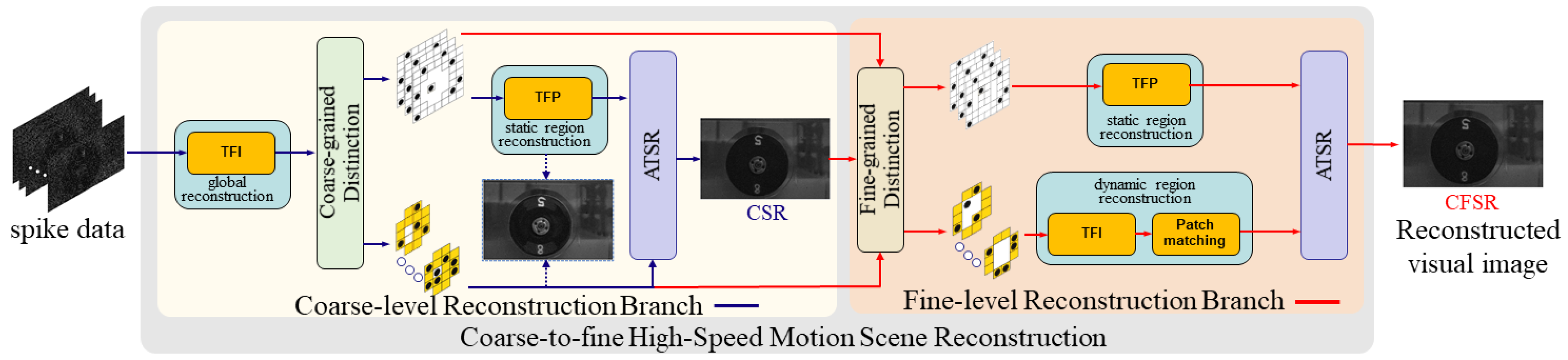
In order to improve the scene reconstruction performance, the retina-like visual image reconstruction framework via a spiking neural model has been proposed to distinguish the dynamic and static spikes and reconstruct the image by using a dynamic neuron extraction model [24]. The local motion excitation layer models the spike data as a motion confidence matrix according to the historical firing distribution, abstracts the spike states into the first-order Markov random field with binary labels [29], and marks each output spike as dynamic or static based on the graph cuts to distinguish the state of the neuron. Then, a spike refining layer sets different refractory periods for dynamic and static neurons to eliminate the noise and preserve the high dynamic range. Finally, a visual reconstruction layer utilizes the spike-timing-dependent plasticity (STDP) learning rule [30] and threshold adaptation [31] to reconstruct the dynamic and static scenes simultaneously.

However, the dynamic scenes reconstruction could still generate motion blur due to the texture from the adaptive threshold (TFA) method, and the STDP learning rule requires a large amount of datasets and time cost. In this paper, we propose a new framework to distinguish the dynamic and static spikes and a new way to reconstruct the images. Experimental results illustrate that our method is superior to SNM in both time complexity and reconstruction results.

To address the aforementioned problem, we propose a CFSR method to reconstruct dynamic and static scenes with region-adaptive-based spike distinction. At the coarse-grained level, we distinguish real-time spikes into dynamic and static regions according to the distribution characteristics of spikes from the input spike data in fixed time, and then we take advantages of the TFI and TFP methods to reconstruct high-speed and stationary scenes, respectively. The reconstructions of two regions are fused to obtain the coarse-grained results. Based on the coarse-grained reconstructions and the distinguished spikes, we perform these major operations, including the fine-grained spikes distinction, the region-based reconstruction, and the fusion at the fine-grained level to additionally distinguish the spikes for further image reconstruction. Furthermore, the difference between adjacent inter-spike intervals (DAISI) and the background subtraction [32] are utilized for the fine-grained distinction. The patch matching method is integrated along with the TFI for dynamic region reconstruction, which is fused with the static region scene reconstruction via the TFP method to obtain the final reconstruction. Finally, our coarse-to-fine scene reconstruction can obtain better image quality and motion details with lower noise and less blur.

3. The CFSR Method

3.1. The Coarse-to-Fine High-Speed Motion Scene Reconstruction Framework

To address the challenge of high-speed motion scene reconstruction from the spike data, we propose a novel spike-based CFSR model. The overall architecture of the spike-based CFSR model is illustrated in Figure 1.

We first take the traditional TFI method for the input spike data for the global reconstruction. Then, we take the coarse-grained distinction to distinguish the spike state adaptively according to the input spike data to output a spike train with binary marks (dynamic or static), which are marked by the dynamic or static state.

We take the TFP to reconstruct the static spikes and fuse them with the reconstruction via the TFI method to reconstruct the intermediate motion scene denoted by the CSR via the adaptive threshold scene reconstruction (ATSR). Moreover, we propose a fined-grained distinction to further distinguish the spike state and use the patch matching method [33] to refine the dynamic region reconstruction. Finally, the dynamic and static reconstruction results are fused to obtain the final reconstructed scene denoted by the CFSR via the ATSR method. The details of the coarse-grained reconstruction and the fine-grained reconstruction are described in Section 3.2 and Section 3.3, respectively .

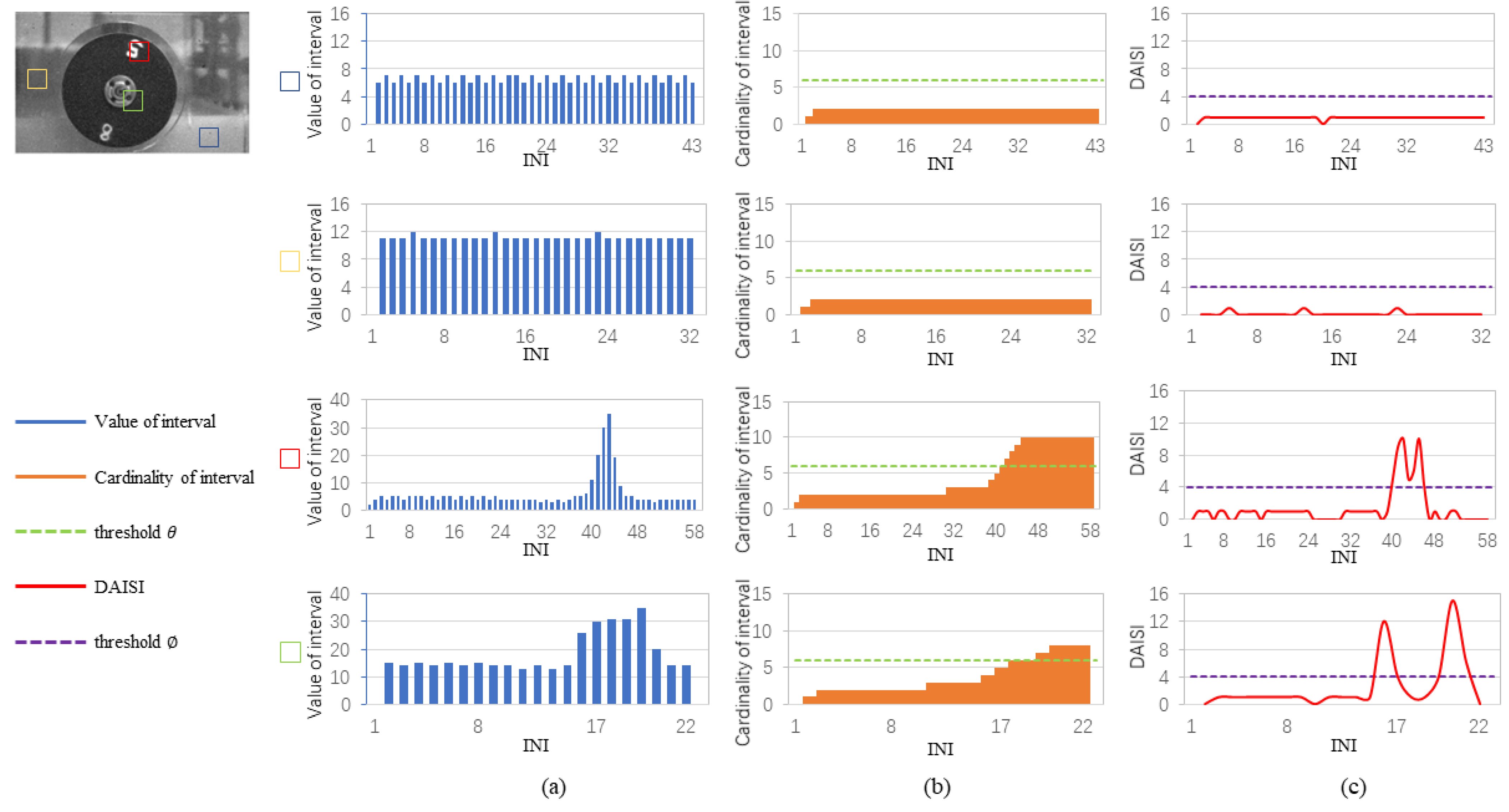
3.2. Coarse-Grained Reconstruction

For the input raw spike data, we first use the TFI method for global reconstruction and distinguish the spikes in a coarse-grained level. We exploit the spatial distribution for ISI to guide the coarse-grained distinction process. As shown in Figure 2a, we observe that there are different numbers and values of ISI within a fixed time interval T, which is formulated as a set,

$$T={\left.{\left\{\Delta t\right.}_m\right\}}_{m=1}^n,$$

(5)

where n denotes the number of ISI in the set T, and $\Delta t_m$ is the m-th inter-spike interval in the fixed time interval T.

Given a fixed time interval T, the cardinality of the set T are not identical. As shown in Figure 2b, when the pixel belongs to the static region, each ISI value in the ${\left.{\left\{\Delta t\right.}_m\right\}}_{m=1}^n$ is relatively average. However, the differences of all the ISI values ${\left.{\left\{\Delta t\right.}_m\right\}}_{m=1}^n$ for the dynamic region are large.Thus, the cardinality of the set T in the dynamic region is larger than that in the static region. Therefore, we distinguish the dynamic and static regions coarsely by

$$M_{t_m}\left(x,y\right)=\left\{\begin{array}{c}1\left|{\left.{\left\{\Delta t\right.}_m\right\}}_{m=1}^n\right|\ge \theta \\ 0\left|{\left.{\left\{\Delta t\right.}_m\right\}}_{m=1}^n\right|<\theta ,\end{array}\right.$$

(6)

where $\theta$ represents the predetermined threshold, and $\left|•\right|$ is the cardinality of a given set. $M_{t_m}\in \left\{0,1\right\}$ is a binary matrix denoting the states of the spike, where the value 1 denotes that the pixel (x, y) belongs to the dynamic region at moment $t_m$. The real-time spike can be marked as static and dynamic states adaptively by Equation (6). In addition, the range of $\theta$ depends on n, and the size of n is related to time and light intensity. We empirically set the threshold $\theta$.

For the dynamic and static regions after coarse-grained spike state distinction, we use different characteristics of the static and dynamic regions for image reconstruction. The TFI method (3) and the TFP method (4) mentioned in Section 2.2 are utilized for the dynamic region reconstruction and static region reconstruction, respectively, as shown in Figure 1.

After the static and dynamic region reconstruction, to keep the consistency of brightness of the two states reconstruction we adopt an adaptive threshold scene reconstruction (ATSR) step to fuse the static and dynamic region reconstruction. We calculate the average brightness ratio of the reconstructions of static regions via the TFP and TFI methods as the adaptive threshold to adjust the brightness of the static region reconstruction via the TFP method,

$${S^{\prime }}_{TFP}(x,y)=S_{TFP}(x,y)·\sum _{(x,y)\in R}\left(S_{TFI}\left(x,y\right)/S_{TFP}(x,y)\right)/N,$$

(7)

where R represents the static region of the reconstruction image, S is the value of static region of the reconstruction, and $S_{TFP}$ represents the value of the static region of the reconstruction by the TFP method. N is the number of spikes in the region R.

Here, the scene reconstruction of static regions is also performed by the TFI method as a guide to obtain the adaptive threshold. After multiplying by the adaptive threshold, the brightness value of the static region via the TFP method is adjusted to be as consistent as possible with that of the dynamic region. Thus, we can obtain the fused scene. In addition, the adaptive threshold is also adopted in the ATSR of the fined-grained reconstruction.

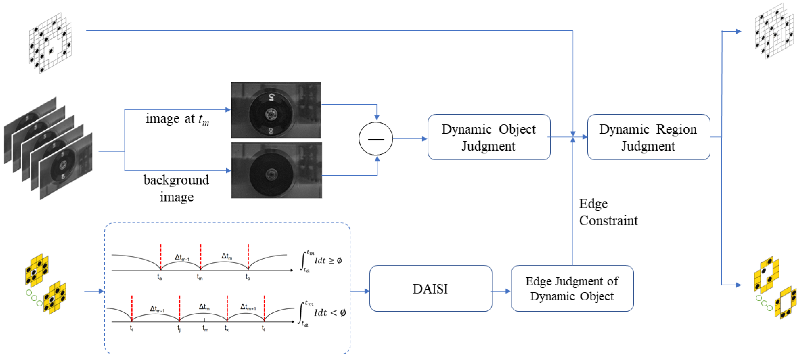
3.3. Fine-Grained Reconstruction

As shown in Figure 2c, the difference between adjacent inter-spike intervals (DAISI) of the static and dynamic regions are also different. After coarse-grained reconstruction, the fine-grained distinction is operated on the dynamic spikes and the coarse-grained scene reconstruction, as illustrated in Figure 3. We can first obtain the coarse-grained reconstruction scene $f_{t_m}\left(x,y\right)$ of consecutive frames in the fixed time interval T. We utilize the Mixture of Gaussian model (MOG) based background subtraction method [32] to distinguish the moving object from the dynamic region to obtain the background image $B\left(x,y\right)$. Then, we can calculate the differential image $D_{t_m}^{\prime }\left(x,y\right)$ via

$$D_{t_m}^{\prime }\left(x,y\right)=\left|f_{t_m}\left(x,y\right)-B(x,y)\right|.$$

(8)

We set a threshold ${\phi }_0$ and obtain the binary image $R_{t_m}^{\prime }\left(x,y\right)$ by the threshold processing for the differential image $D_{t_m}^{\prime }\left(x,y\right)$,

$$R_{t_m}^{\prime }\left(x,y\right)=\left\{\begin{array}{c}1D_{t_m}^{\prime }\left(x,y\right)\ge {\phi }_0\\ 0D_{t_m}^{\prime }\left(x,y\right)<{\phi }_0.\end{array}\right.$$

(9)

The values of 1 and 0 represent the dynamic object and the static region, respectively.

However, the distinction of the edge of the dynamic object is not well-defined. We then use the difference between adjacent inter-spike intervals (DAISI) to judge the edge of the dynamic object. We observe that when the average brightness intensity changes greatly in a short time, the current spikes are the edge of the dynamic region, assuming that the brightness of the dynamic region is inconsistent with that of the static region, as shown in Figure 2c. There is an edge of the dynamic region when a change in that log average luminance intensity ${\overline{I}}_m$ of $\Delta t_m$ exceeds a threshold $\delta$,

$$\left|\log \left({\stackrel{-}{I}}_m\right)-\log \left({\stackrel{-}{I}}_{m-1}\right)\right|\ge \delta ,$$

(10)

where ${\overline{I}}_m$ and ${\overline{I}}_{m-1}$ can be estimated by Equation (2). Correspondingly, the edge of the dynamic region exists when a change in the log ISI exceeds a threshold $\phi$,

$$\left|\log \left({\Delta t}_m\right)-\log \left({\Delta t}_{m-1}\right)\right|\ge \phi .$$

(11)

When a spike is generated at time $t_m$, Equation (10) can represent the motion state at the current time well, as shown in Figure 3. However, when there is no spike generated at time $t_m$, we have difficulty judging the motion state at the current moment $t_m$ by the difference between two adjacent ISIs, as shown in Figure 3. For this case, we utilize the difference among three adjacent ISIs to judge the edge of the moving region via

$$\left\{\left|\log \left({\Delta t}_m\right)-\log \left({\Delta t}_{m-1}\right)\right|\bigcap \left|\log \left({\Delta t}_m\right)-\log \left({\Delta t}_{m+1}\right)\right|\right\}\ge \phi .$$

(12)

Assume $t_a$ is the time point when the spike is generated before $t_m$. We can assess whether a one-bit spike is generated or not from $t_a$ to $t_m$ via Equation (1). Thus, we formulate the difference image $D_{t_m}\left(x,y\right)$ of the spike data at time $t_m$ in the case of Figure 3 as follows,

$$D_{t_m}\left(x,y\right)=\left\{\begin{array}{c}\begin{array}{cc}\left|\log \left({\Delta t}_m\left(x,y\right)\right)-\log \left({\Delta t}_{m-1}\left(x,y\right)\right)\right|& {\int }_{t_a}^{t_m}Idt\ge \varnothing \end{array}\\ \begin{array}{cc}\left(\genfrac{}{}{0pt}{}{\left|\log \left({\Delta t}_m\left(x,y\right)\right)-\log \left({\Delta t}_{m-1}\left(x,y\right)\right)\right|}{\bigcap \left|\log \left({\Delta t}_m(x,y)\right)-\log \left({\Delta t}_{m+1}(x,y)\right)\right|}\right)& {\int }_{t_a}^{t_m}Idt<\varnothing .\end{array}\end{array}\right.$$

(13)

The threshold $\phi$ in Equations (11) and (12) is a predetermined set, and the binary processing is performed on the pixel points one by one to obtain the binary image $R_{t_m}\left(x,y\right)$. The values of 1 and 0 are set to indicate the edge of the dynamic object and the static region

$$R_{t_m}\left(x,y\right)=\left\{\begin{array}{c}1D_{t_m}\left(x,y\right)\ge \phi \\ 0D_{t_m}\left(x,y\right)<\phi .\end{array}\right.$$

(14)

Finally, the edge information obtained by the DAISI method is used to refine the edge of the dynamic object. Thus, the dynamic and static spikes by the fine-grained distinction are obtained.

Different from the coarse-grained reconstruction, after using the TFI method for the dynamic region reconstruction, the PatchMatch method [33] is utilized to preserve the local structure and visual richness of textures as well as to eliminate the noise and enhance the moving object detail. For each patch of the given $f_{t_m}\left(x,y\right)$ , the most similar patch in each of the adjacent frames ${\left.{\left\{f\right.}_t\left(x,y\right)\right\}}_{t=t_m\pm 5i}$, where $i=\left\{1,2,3,\dots N\right\},N=10$, has a size $6\times 6$, obtained by the PatchMatch method [33]. The patches of the dynamic region are overlapped extracted to prevent blocking artifacts, and we take the average of all candidates as the output pixel value. Finally, the ATSR step is also utilized to guarantee the consistency of brightness of final scene reconstruction.

4. Experiment Results

4.1. Experimental Setting

Our CFSR framework was implemented by the publicly available Matlab (version 2019a), Python (version 2.7), and Brian2 (version 2.2.2.1) on an AMD Ryzen 7 5800H-GPU system. To demonstrate the CFSR framework, we used the PKU-SPIKE-RECON dataset [6,8] from Peking University, including spike sequences captured by the spike camera. This dataset contains eight sequences including two categories of normal speed (Class A) and high speed (Class B) scenarios. Each sequence was captured by the spike camera with 40,000 Hz sampling rate. The experiments were conducted on three spike sequences captured from high-speed scenes, including “Rotation1”, “Rotation2” and “Car”, as shown in Figure 4. Among them, “Car” describes a car traveling at a speed of 100 km/h (kilometers per hour). The sequence “Rotation1” describes a disk with 2000 rpm (revolutions per minute), and the sequence “Rotation2” depicts an electric fan with 2600 rpm [18]. The resolution of these three high-speed scenes is of size 400 × 250 × 2000. According to our previous statistics, we set T = 400, $\theta$ = 6, ${\phi }_0$ = 50, $\phi$ = 4, and ∅ = 12, respectively. To evaluate the performance of our CFSR method on reconstructing high-speed moving scenes, we compared it with three conventional texture reconstruction methods, including “Texture from ISI (TFI)”, “Texture from Playback (TFP)” (w = 160), and a spiking neural model [8].

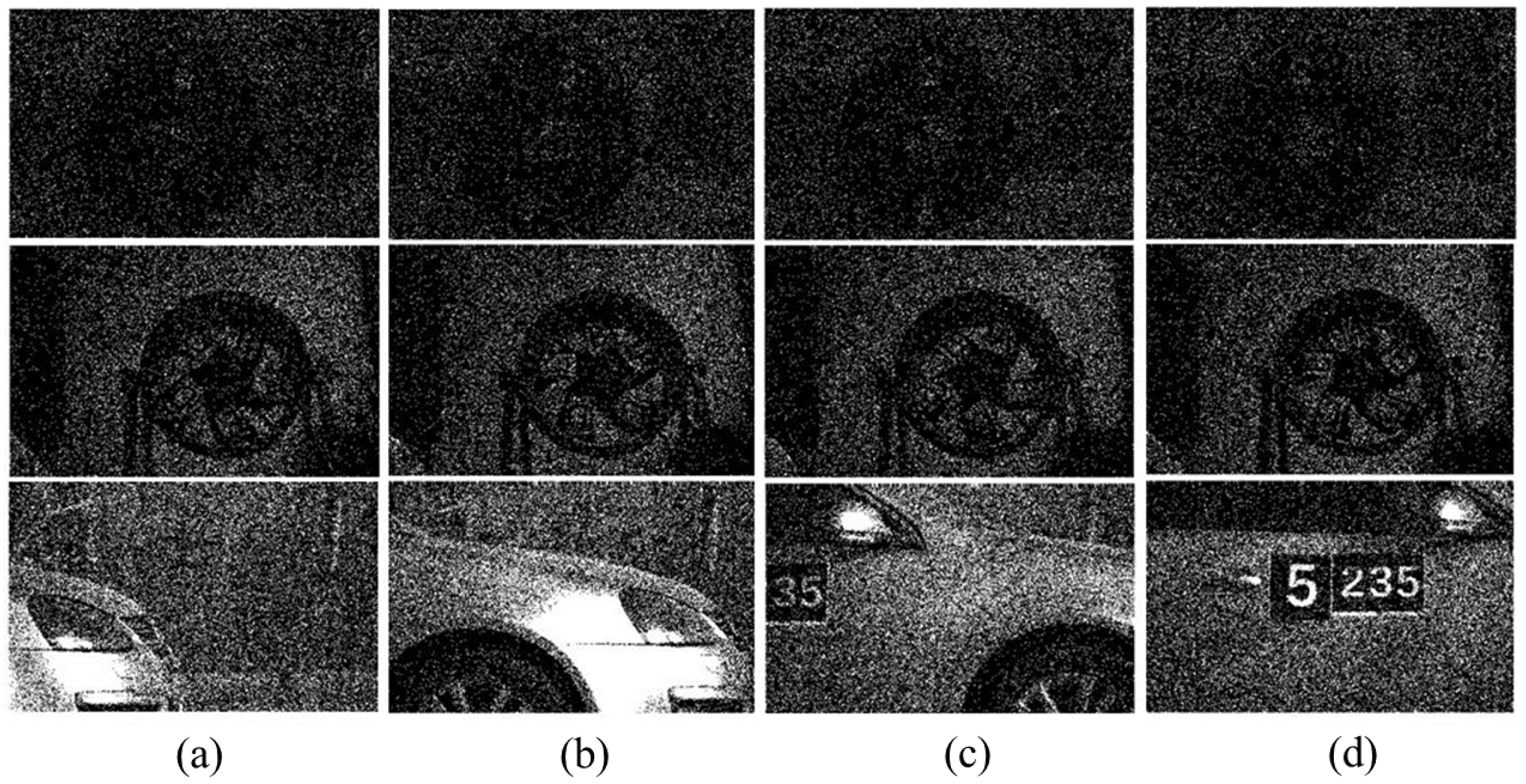
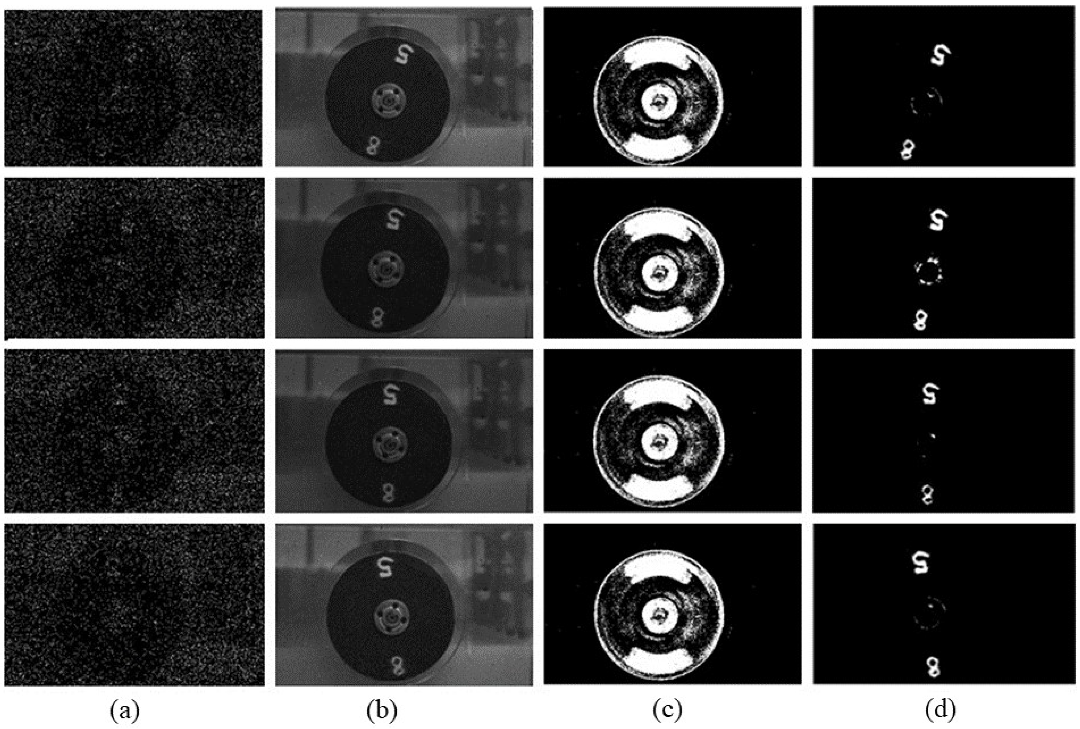
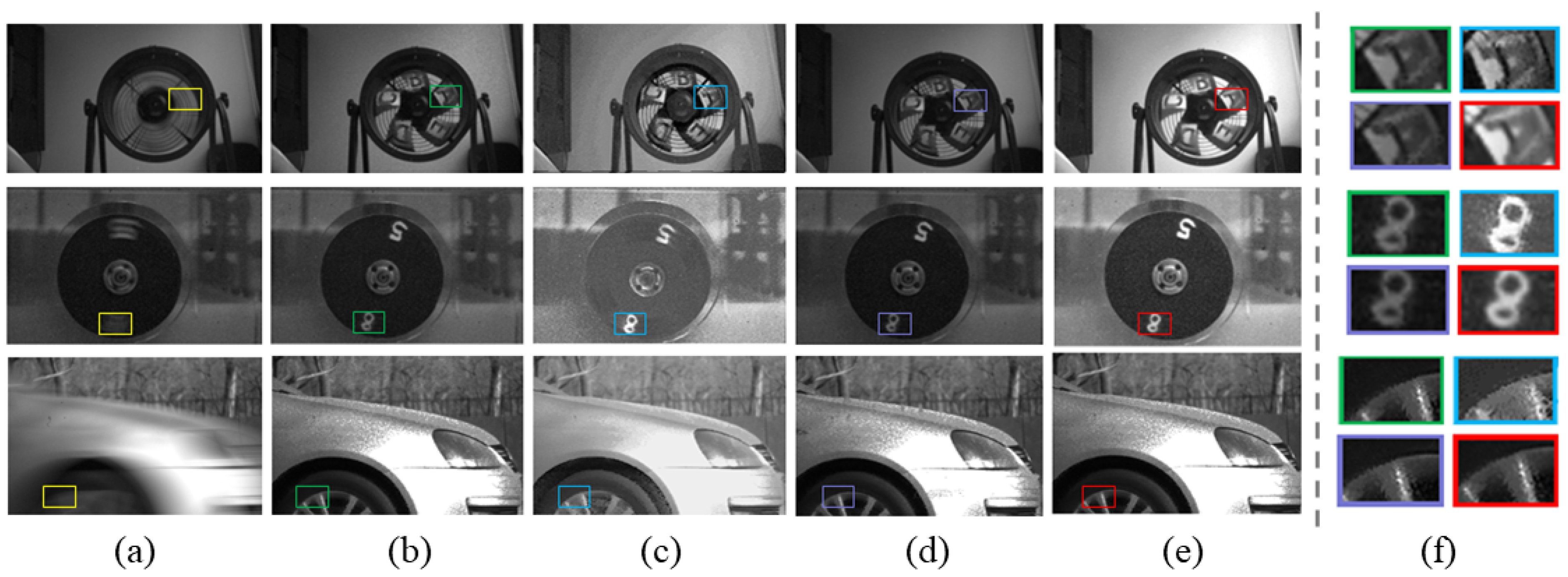
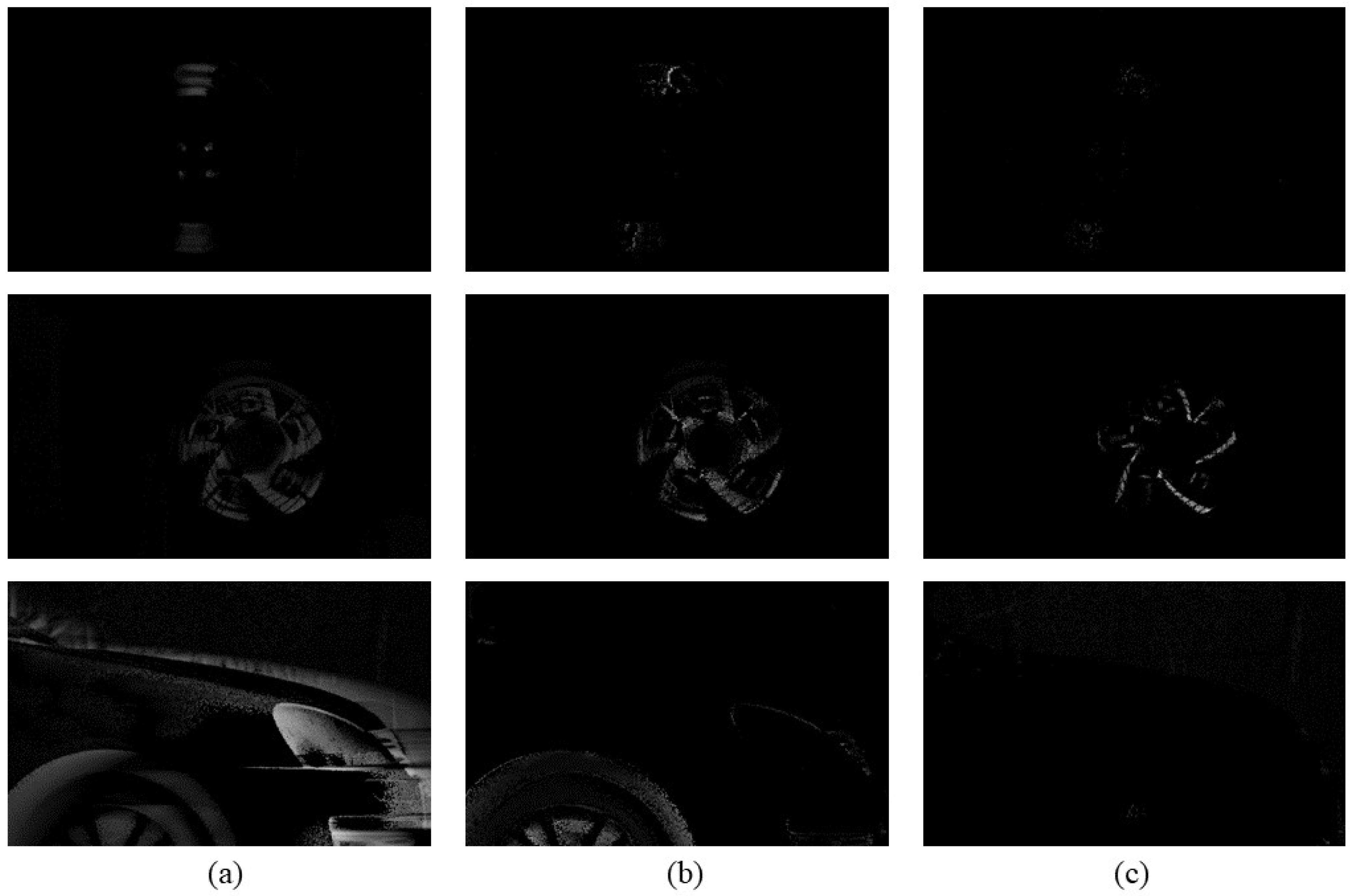
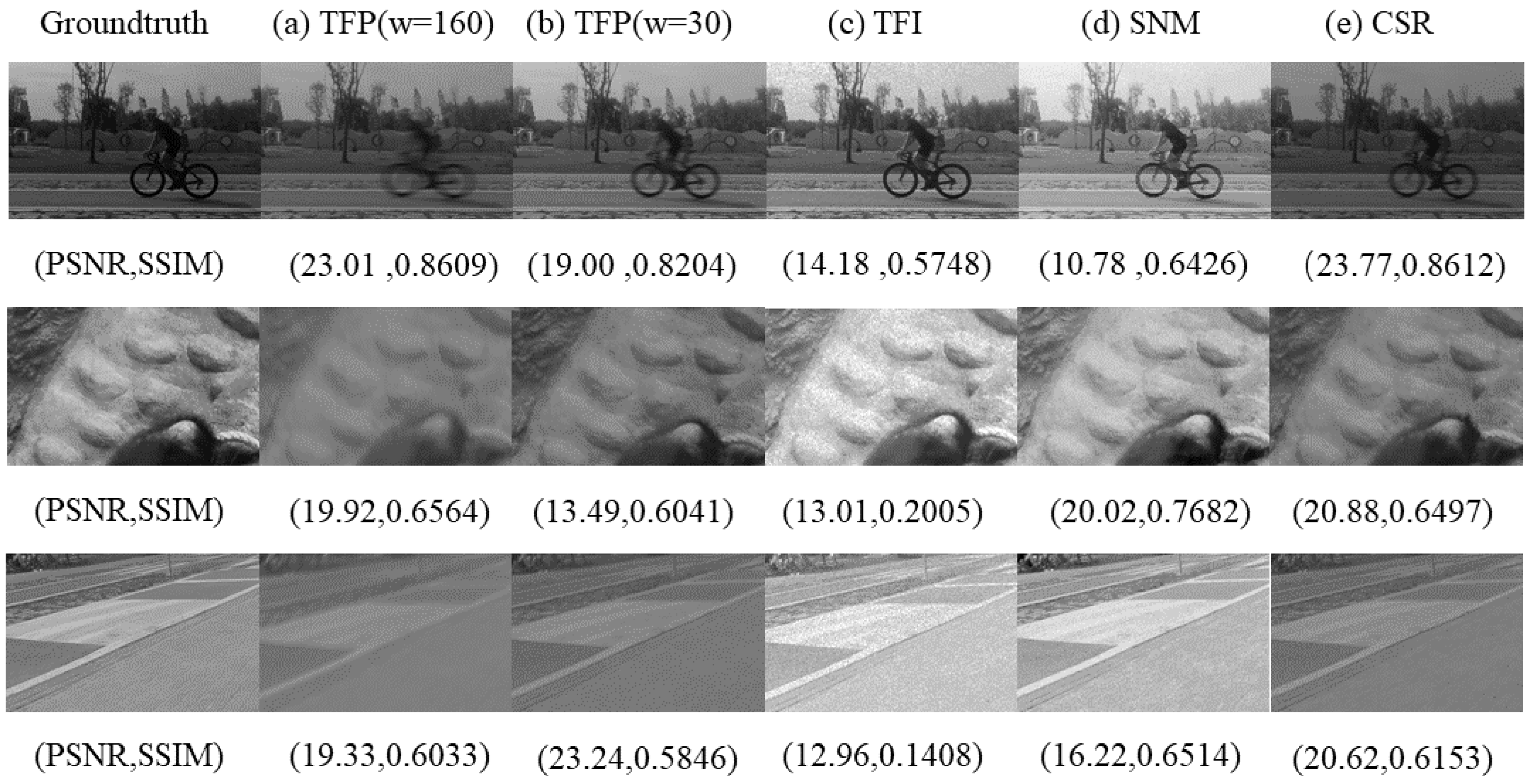
4.2. Visual Texture Reconstruction

Spike Distinction. In our CFSR, the spikes <are distinguished into dynamic and static regions by RASD, including coarse-grained and fine-grained distinctions. We compared our spike distinction method with raw spike and TFI [20]. As shown in Figure 5, static and dynamic regions can be roughly distinguished, where the pixels belong to static regions are marked as the dynamic due to high speed. The dynamic and static regions with the fine-grained distinction can be further distinguished; thus, the dynamic region for each frame with the fine-grained method is marked more accurately than that of coarse-grained.

Visual Quality. We compared our CFSR with three methods, namely, the TFI [20], TFP [18], and a spiking neural model [24]. The first two methods are retina-inspired sampling methods, and the last method is a spiking neural network learning method. As shown in Figure 6, the reconstructed image by the TFI can reconstruct the outline of fast-moving objects well but with some noise, artifact, and ghosts. To see more clearly, we also present the difference images of the TFP and SNM methods and our proposed CFSR method compared with the TFI reconstruction, as shown in Figure 7. The TFP method can improve the performance but still suffers severe motion blur on dynamic regions, which also influences the visual performance. The spiking neural model (SNM) can promote the image quality in both static and dynamic regions; however, the dynamic regions reconstruction still suffers some motion blur. In contrast, our CFSR method can outperform other methods and generate the best results with lower noise, less blur, higher image quality and richer details.

Quantitative Evaluation. We also evaluated our proposed CFSR using an image quality assessment metric standard deviation (STD) and a no-reference image blur metric called CPBD [34] on the consecutive 200 frame raw spikes from the PKU-SPIKE-RECON dataset for quantitative comparison. The STD is related to the contrast of the image; it can be computed as $STD=\sqrt{\frac{{\sum }_{x=1}^H{\sum }_{y=1}^W{\left(I_{\left(x,y\right)}-\overline{I}\right)}^2}{\left(H-1\right)\left(W-1\right)}}$, where H and W represent the width and length of the reconstructed image, $I_{\left(x,y\right)}$ is the gray value of the pixel $\left(x,y\right)$, and $\overline{I}$ is the sample mean. Larger standard deviation (STD) values mean higher contrast. CPBD was used to measure the motion blur. From the probability density function of detecting blur, the cumulative probability of blur detection was calculated as $CPBD={\sum }_{P_{BLUR}=0}^{P_{BLUR}=P_{JNB}}P\left(P_{BLUR}\right)$, where $P_{BLUR}=1-exp(-{\left|\frac{w\left(e_i\right)}{w_{JNB}\left(e_i\right)}\right|}^{\beta })$, $w\left(e_i\right)$ is the measured width of the each edge $e_i$, $w_{JNB}\left(e_i\right)$ is the “just noticeable blur” (JNB) [35] width, which depends on the local contrast C in the neighborhood of edge $e_i$, and $\beta$ is a parameter whose value is obtained by means of least squares fitting. $P\left(P_{BLUR}\right)$ denotes the value of the probability distribution function at a given $P_{BLUR}$. At the JNB, $w\left(e_i\right)=w_{JNB}\left(e_i\right)$, which corresponds to the probability of blur detection $P_{BLUR}=P_{JNB}=63$%. Higher CPBD means less blur and vice versa. As listed in

Table 1. The STD and CPBD metrics of the PKU-SPIKE-RECON dataset by different methods. Red and blue indicate the best and the second best performance, respectively.

Metric	Method	Rotation1	Rotation2	Car	Mean
	TFI [18]	25.1455	40.1673	53.6904	39.6677
	TFP [20]	23.5241	35.9377	43.6953	34.3858
	SNM [24]	39.9200	60.2485	58.1364	52.7683
	CSR	24.3537	37.6037	55.8144	39.2573
STD	CFSR	50.6763	75.0012	68.4223	64.6998
	TFI	0.9101	0.8189	0.9572	0.8954
	TFP	0.8115	0.6153	0.5075	0.6448
	SNM	0.8254	0.6376	0.6511	0.7041
	CSR	0.8811	0.6781	0.7564	0.7719
CPBD [34]	CFSR	0.9262	0.6905	0.8109	0.8092

, our CSFR outperformed other state-of-the-art methods in terms of STD. Compared to the SNM method, our CFSR model had a 22.61% improvement in terms of STD on average. However, we notice that the CPBD of the TFI outperformed other methods due to the TFI results with rich texture along with high noise and artifact. Our CSFR method which maintains sharpness and higher contrast, presented the second best performance in all the comparison methods. The 14.92% improvement of CPBD can be achieved by our CSFR model compared with SNM method on average. In summary, our CFSR methods can present appreciable performance.

Furthermore, we also applied the reconstruction methods on a simulated dataset provided by [23], where the spike streams and ground truth images are generated from video-based virtual scenes with the camera’s ego-motion. We compared the TFP, TFI, SNM, and CSR methods against the ground truth for quantitative evaluation. All parameters involved in our method and the competing methods were optimally assigned or selected as suggested in the reference papers. In our method, we set T = 300, $\theta$ = 10, and w = 30, respectively. As shown in Figure 8, the proposed CSR method achieved the best results in terms of PSNR and comparable results with SNM in terms of SSIM.

4.3. Complexity Analysis

Here we evaluate the computational complexity of our method. For comparison, we consider the problem of a reconstructing image from K-frame raw spike data of size $H\times W$. We first discuss the complexity of each pixel in the reconstruction image. In coarse-grained reconstruction, for each pixel, the CSR method only needs to update the fixed time interval T, the number n of ISI in the set T, the number N of spikes in the region R, and the predetermined threshold $\theta$ when a spike generates at that pixel. For the TFI and TFP methods utilized in CSR, the TFI only needs to find the nearest spike to reconstruct the image; thus, the best and the worst case complexity of the TFI are $O\left(1\right)$ and $O\left(logK\right)$, respectively. The complexity of the TFP is $O\left(w\right)$, where w is the time window utilized in TFP. Therefore, the total complexity of the reconstruction methods utilized in CSR is $O\left(logK\right)$. Note that the CSR method needs extra steps to distinquish whether a pixel belongs to the motion region or not by Equation (6). However, it only takes constant time for each pixel. It does not affect the asymptotic time complexity. Therefore, the time complexity of the CSR method is $O\left(HWlogK\right)$ for each frame.

Different from coarse-grained reconstruction, the randomized correspondence algorithm [33], as the patch matching method, is added to fine-grained reconstruction in the dynamic region reconstruction. It takes at most $logR$ steps to find the most similar patch in each of the adjacent frames ${f_t\left(x,y\right)}_{t=t_m\pm 5i}$, where $i=\left\{1,2,3,\dots N\right\},N=10$, where R is the region of fine-grained distinction. Thus, the total complexity of the randomized correspondence algorithm is $O\left(RlogR\right)$. Fine-grained distinction also takes constant time for each pixel, so it does not affect the asymptotic time complexity. Therefore, the total complexity of the CFSR method is $O\left(HWRlog\left(R\right)\right)$ for each frame, and it takes at most $O\left(HWKRlog\left(R\right)\right)$ time to construct a K-frame video from raw spikes.

In comparison, the SNM method in [24] takes at least $O\left(H^3{W}^3\right)$ time to implement a graph cut for each frame; thus, it takes at least $O\left(H^3{W}^{3}K\right)$ time to reconstruct a K-frame video [25]. Therefore, our method achieves a significantly lower time complexity than the state-of-the-art methods.

4.4. Discussion

There are still some limitations in this work, which could be improved. We observe that the brightness of the scenes affects the frequency of the interval of the spike dataset captured by the spike camera. Meanwhile, the inter-spike interval is utilized in spike distinction. Now, the brightness is not considered in our CSFR model. In the future, the region-based distinction with brightness guidance will be studied for further distinguishing the dynamic and static region. Furthermore, although our proposed CFSR framework supports flexible and adaptive ways to reconstruct images, the patch matching method utilized in fine-grained reconstruction spends most of the time in the CFSR framework, which partly restricts the efficiency of our CFSR framework. Therefore, we can further improve the efficiency of the high-speed scene reconstruction. Moreover, the image quality of the reconstruction in the static region by the CFSR method did not reach the image quality captured by the frame-based camera. Motivated by the successful applications of the attention fusion network [12] with the frames and events as well as the unifying framework that bridges the intensity images and neuromorphic event [13], the APS data captured from a frame-based camera as the guidance may also be introduced in the CFSR to further improve the performance of the reconstructed images. As the synthesized dataset is generated with only the camera’s ego-motion, it is unnecessary to further distinguish the static and motion regions, and the fine-grained reconstruction is not required. Our proposed CFSR and CSR can be utilized in high-speed motion and video-based scenes reconstruction captured by a spike camera, respectively.

5. Conclusions

In this paper, we propose a novel CFSR method with the region-adaptive-based spike distinction (RASE) framework to reconstruct visual scenes from spike data. Both coarse-grained and fine-grained reconstructions in our CSFR method include spike distinction, region-based reconstruction, and adaptive threshold scene fusion (ATSF). We utilize the characteristic of the ISI and integrate the DAISI and the background subtraction into the region-adaptive-based spike distinction (RASD) to distinguish the spikes. The TFP is utilized for static region reconstruction and the TFI along with the patch matching method used for dynamic region reconstruction. Finally, the visual scene can be reconstructed by the ATSF. Experimental results demonstrate that our proposed CFSR method can generate visual scene with high quality in terms of low noise, sharp textures, and fine details, which validates the superiority of our CFSR over the competing methods. In future work, our CFSR framework can be further improved by other retina-inspired methods applied for region-based reconstruction.

References

1. Yurtsever, E.; Lambert, J.; Carballo, A.; Takeda, K. A Survey of Autonomous Driving: Common Practices and Emerging Technologies. IEEE Access 2020, 8, 58443–58469. [Google Scholar] [CrossRef]
2. Liu, C.; Huynh, D.Q.; Sun, Y.; Reynolds, M.; Atkinson, S. A Vision-Based Pipeline for Vehicle Counting, Speed Estimation, and Classification. IEEE Trans. Intell. Transp. Syst. 2021, 22, 7547–7560. [Google Scholar] [CrossRef]
3. Sana, F.; Isselbacher, E.M.; Singh, J.P.; Heist, E.K.; Pathik, B.; Armoundas, A.A. Wearable Devices for Ambulatory Cardiac Monitoring. J. Am. Coll. Cardiol. 2020, 75, 1582–1592. [Google Scholar] [CrossRef] [PubMed]
4. Litzenberger, M.; Posch, C.; Bauer, D.; Belbachir, A.N.; Schon, P.; Kohn, B.; Garn, H. Embedded vision system for real-time object tracking using an asynchronous transient vision sensor. In Proceedings of the 2006 IEEE 12th Digital Signal Processing Workshop & 4th IEEE Signal Processing Education Workshop, Teton National Park, WY, USA, 24–27 September 2006; pp. 173–178. [Google Scholar]
5. Gehrig, D.; Rebecq, H.; Gallego, G.; Scaramuzza, D. Asynchronous, photometric feature tracking using events and frames. In Proceedings of the European Conference on Computer Vision (ECCV), Munich, Germany, 8–14 September 2018; pp. 750–765. [Google Scholar]
6. Maqueda, A.I.; Loquercio, A.; Gallego, G.; García, N.; Scaramuzza, D. Event-based vision meets deep learning on steering prediction for self-driving cars. In Proceedings of the IEEE Conference on Computer Vision and Pattern Recognition, Salt Lake City, UT, USA, 18–23 June 2018; pp. 5419–5427. [Google Scholar]
7. Lichtsteiner, P.; Posch, C.; Delbruck, T. A 128 × 128 120 db 15 μs latency asynchronous temporal contrast vision sensor. IEEE J. -Solid-State Circuits 2008, 43, 566–576. [Google Scholar] [CrossRef]
8. Berner, R.; Brandli, C.; Yang, M.; Liu, S.; Delbruck, T. A 240 × 180 10 mw 12 μs latency sparse-output vision sensor for mobile applications. In Proceedings of the 2013 Symposium on VLSI Circuits, Kyoto, Japan, 12–14 June 2013; pp. C186–C187. [Google Scholar]
9. Hu, Y.; Liu, H.; Pfeiffer, M.; Delbruck, T. Dvs benchmark datasets for object tracking, action recognition, and object recognition. Front. Neurosci. 2016, 10, 405. [Google Scholar] [CrossRef] [PubMed]
10. Barranco, F.; Fermuller, C.; Aloimonos, Y.; Delbruck, T. A dataset for visual navigation with neuromorphic methods. Front. Neurosci. 2016, 10, 49. [Google Scholar] [CrossRef] [PubMed]
11. Binas, J.; Neil, D.; Liu, S.C.; Delbruck, T. Ddd17: End-to-end davis driving dataset. arXiv 2017, arXiv:1711.01458. [Google Scholar]
12. Liu, M.; Qi, N.; Shi, Y.; Yin, B. An Attention Fusion Network For Event-Based Vehicle Object Detection. In Proceedings of the 2021 IEEE International Conference on Image Processing (ICIP), Anchorage, AK, USA, 19–22 September 2021; pp. 3363–3367. [Google Scholar] [CrossRef]
13. Wang, Z.W.; Duan, P.; Cossairt, O.; Katsaggelos, A.; Huang, T.; Shi, B. Joint Filtering of Intensity Images and Neuromorphic Events for High-Resolution Noise-Robust Imaging. In Proceedings of the 2020 IEEE/CVF Conference on Computer Vision and Pattern Recognition (CVPR), Seattle, WA, USA, 13–19 June 2020; pp. 1606–1616. [Google Scholar] [CrossRef]
14. Brandli, C.; Berner, R.; Yang, M.; Liu, S.C.; Delbruck, T. A 240 × 180 130 db 3 μs latency global shutter spatiotemporal vision sensor. IEEE J. Solidst. Circ. 2014, 49, 2333–2341. [Google Scholar] [CrossRef]
15. Posch, D.M.C.; Wohlgenannt, R. An asynchronous time-based image sensor. In Proceedings of the IEEE International Symposium on Circuits and Systems, Geneva, Switzerland, 28–31 May 2000; pp. 2130–2133. [Google Scholar]
16. Gould, S.; Arfvidsson, J.; Kaehler, A.; Sapp, B.; Messner, M.; Bradski, G.; Baumstarck, P.; Chung, S.; Ng, A.Y. Arfvidsson, Peripheral-foveal vision for real-time object recognition and tracking in video. In International Joint Conference on Artificial Intelligence; Morgan Kaufmann Publishers, Inc.: San Francisco, CA, USA, 2007. [Google Scholar]
17. Zhao, J.; Yu, Z.; Ma, L.; Ding, Z.; Zhang, S.; Tian, Y.; Huang, T. Modeling The Detection Capability of High-Speed Spiking Cameras. In Proceedings of the ICASSP 2022—2022 IEEE International Conference on Acoustics, Speech and Signal Processing (ICASSP), Singapore, 23–27 May 2022; pp. 4653–4657. [Google Scholar] [CrossRef]
18. Dong, S.; Huang, T.; Tian, Y. Spike camera and its coding methods. In Proceedings of the Data Compression Conference, (DCC), Snowbird, UT, USA,, 4–7 April 2017; p. 437. [Google Scholar]
19. Dong, S.; Zhu, L.; Xu, D.; Tian, Y.; Huang, T. An efficient coding method for spike camera using inter-spike intervals. In Proceedings of the Data Compression Conference, (DCC), Snowbird, UT, USA, 26–29 March 2019; p. 568. [Google Scholar]
20. Zhu, L.; Dong, S.; Huang, T.; Tian, Y. A retina-inspired sampling method for visual texture reconstruction. In Proceedings of the 2019 IEEE International Conference on Multimedia and Expo (ICME), Shanghai, China, 8–12 July 2019; pp. 1432–1437. [Google Scholar]
21. Culurciello, E.; Cummings, R.E.; Boahen, K.A. A biomorphic digital image sensor. IEEE J. -Solid-State Circuits 2003, 38, 281–294. [Google Scholar] [CrossRef]
22. Zhao, J.; Xiong, R.; Zhao, R.; Wang, J.; Ma, S.; Huang, T. Motion Estimation for Spike Camera Data Sequence via Spike Interval Analysis. In Proceedings of the 2020 IEEE International Conference on Visual Communications and Image Processing (VCIP), Macau, China, 1–4 December 2020; pp. 371–374. [Google Scholar] [CrossRef]
23. Zhao, J.; Xiong, R.; Liu, H.; Zhang, J.; Huang, T. Spk2ImgNet: Learning to Reconstruct Dynamic Scene from Continuous Spike Stream. In Proceedings of the 2021 IEEE/CVF Conference on Computer Vision and Pattern Recognition (CVPR), Nashville, TN, USA, 19–25 June 2021; pp. 11991–12000. [Google Scholar] [CrossRef]
24. Zhu, L.; Dong, S.; Li, J.; Huang, T.; Tian, Y. Retina-like visual image reconstruction via spiking neural model. In Proceedings of the IEEE/CVF Conference on Computer Vision and Pattern Recognition, Seattle, WA, USA, 13–19 June 2020. [Google Scholar]
25. Zheng, Y.; Zheng, L.; Yu, Z.; Shi, B.; Tian, Y.; Huang, T. High-speed Image Reconstruction through Short-term Plasticity for Spiking Cameras. In Proceedings of the IEEE/CVF Conference on Computer Vision and Pattern Recognition, Nashville, TN, USA, 20–25 June 2021. [Google Scholar]
26. Hu, Z.; Lu, G.; Guo, J.; Liu, S.; Jiang, W.; Xu, D. Coarse-to-fine Deep Video Coding with Hyperprior-guided Mode Prediction. In Proceedings of the 2022 IEEE/CVF Conference on Computer Vision and Pattern Recognition (CVPR), New Orleans, LA, USA, 19–20 June 2022; pp. 5911–5920. [Google Scholar]
27. Ranjan, A.; Black, M.J. Optical flow estimation using a spatial pyramid network. In Proceedings of the IEEE Conference on Computer Vision and Pattern Recognition, Honolulu, HI, USA, 21–26 July 2017; pp. 4161–4170. [Google Scholar]
28. Gollisch, T.; Markus, M. Rapid neural coding in the retina with relative spike latencies. Science 2008, 319, 1108–1111. [Google Scholar] [CrossRef] [PubMed]
29. Geman, S.; Geman, D. Stochastic relaxation, gibbs distributions, and the bayesian restoration of images. IEEE Trans. Pattern Anal. Mach. Intell. 1984, 6, 721–741. [Google Scholar] [CrossRef] [PubMed]
30. Bi, G.; Poo, M. Synaptic modifications in cultured hippocampal neurons: Dependence on spike timing, synaptic strength, and postsynaptic cell type. J. Neurosci. 1998, 18, 10464–10472. [Google Scholar] [CrossRef] [PubMed]
31. Diehl, P.U.; Cook, M. Unsupervised learning of digit recognition using spike-timing-dependent plasticity. Front. Comput. Neurosci. 2015, 9, 99. [Google Scholar] [CrossRef] [PubMed]
32. Stauffer, C.; Grimson, W. Adaptive background mixture models for real-time tracking. In Proceedings of the 1999 IEEE Computer Society Conference on Computer Vision and Pattern Recognition, Fort Collins, CO, USA, 23–25 June 1999; pp. 246–252. [Google Scholar]
33. Barnes, C.; Shechtman, E.; Finkelstein, A.; Goldman, D.B. PatchMatch: A Randomized Correspondence Algorithm for Structural Image Editing. ACM Trans. Graph 2009, 28, 24. [Google Scholar] [CrossRef]
34. Liu, L.; Hua, Y.; Zhao, Q.; Huang, H.; Bovik, A.C. Blind image quality assessment by relative gradient statistics and adaboosting neural network. Signal Process. Image Commun. 2016, 40, 1–15. [Google Scholar] [CrossRef]
35. Ferzli, R.; Karam, L.J. A No-Reference Objective Image Sharpness Metric Based on the Notion of Just Noticeable Blur (JNB). IEEE Trans. Image Process. 2009, 18, 717–728. [Google Scholar] [CrossRef] [PubMed]
Figure 1. The overall architecture of the spike-based CFSR framework. The coarse-grained reconstruction branch is denoted by dark blue lines. The input is spike data and the outputs are spike train with binary marks (dynamic or static) and the CSR, which are the inputs of the fine-level reconstruction branch denoted by the red lines. The image with the blue wire frame is the intermediate result fused by the results of the TFP and TFI methods directly.
Applsci 13 02424 g001
Figure 2. The temporal distribution of index of number of ISI (INI) under different brightness and motion state. From left to right: (a) value of interval; (b) cardinality of interval; (c) the difference between adjacent inter-spike intervals (DAISI). From top to bottom, the results of different regions are marked in different colors, where the red and gray belong to the dynamic, and the yellow and blue ones are the static, respectively.
Applsci 13 02424 g002
Figure 3. Fine-grained spike state distinction for the dynamic region and the static region. Spike train with binary marks (dynamic or static) and the CSR are as inputs to the fine-grained distinction. The Mixture of Gaussian model (MOG) based background subtraction method is utilized on the CSR for dynamic object judgment, and the difference between adjacent inter-spike intervals (DAISI) is utilized to judge the edge of the dynamic object. Finally, the edge information obtained by the DAISI method is used to refine the dynamic and static spikes.
Applsci 13 02424 g003
Figure 4. Examples of raw spikes presented in the PKU-SPIKE-RECON dataset. From top to bottom: raw spike of the high scenes of ‘Rotation1’, ‘Rotation2’ and ‘Car’, respectively; From left to right of the first two rows: (a) the 100th, (b) 150th, (c) 200th, and (d) 250th frame of ‘Rotation1’ and ‘Rotation2’, respectively. Those of the last row are (a) the 1000th, (b) 1500th, (c) 2000th, and (d) 2500th frame of ‘car’, respectively.
Applsci 13 02424 g004
Figure 5. Comparison of the coarse-grained and fine-grained distinctions with raw spike and the TFI result. From left to right: (a) raw spike; (b) the reconstruction by the TFI; (c) the coarse-grained distinction; and (d) the fine-grained distinction. The white and black value in both (c,d) represent the dynamic and static regions, respectively.
Applsci 13 02424 g005
Figure 6. Visual quality comparison of texture reconstruction by the TFP, the TFI, and the spiking neural model and our proposed method. From left to right: (a) TFP (w = 160); (b) TFI; (c) spiking neural model; (d) coarse-grained reconstruction; (e) fine-grained reconstruction; (f): closeups of the reconstructed results on each method, respectively.
Applsci 13 02424 g006
Figure 7. Different images of the reconstructions of the TFP, SNM, and our CFSR with the TFI. From left to right: (a) TFP (w = 160); (b) SNM; (c) CFSR. The larger the white areas on the image, the larger the difference. The results of our CFSR are with less noise and motion blur in the static and dynamic region, respectively.
Applsci 13 02424 g007
Figure 8. Comparison among different reconstruction methods on synthetic data. From left to right: ground truth, (a) TFP (w = 160); (b) TFP (w = 30); (c) TFI; (d) SNM; (e) CSR (w = 30, θ = 10 ). The PSNR and SSIM of the reconstructed images are also listed below the images, respectively.
Applsci 13 02424 g008