Upper-Bound Limit Analysis of Ultimate Pullout Capacity of Expanded Anchor Cable

Abstract

Expanded anchor cables have been widely used in the rapid development of underground engineering. However, there are still some deficiencies in the computation of the ultimate bearing capacity of expanded anchor cables. Based on the upper-bound theorem of limit analysis, the upper-bound solution of the ultimate bearing capacity of an expanded anchor cable was derived. For this calculation, the instability mechanism of the soil at the front surface of the anchorage segment of the expanded anchor cable was assumed to satisfy the logarithmic spiral failure model, its 3D velocity discontinuity surface was generated using the spatial discretization technique, and the optimal solution was determined through the particle swarm optimization (PSO) algorithm. The breakage mechanism of the anchorage side surface was assumed to appear at the interface between the anchorage body and the soil, and its velocity field satisfied the requirements of the associated flow rule. The accuracy of the proposed analytical solution was well-verified through a comparison with three-dimensional numerical simulations, and its superiority was also well-demonstrated in comparison to the existing theoretical calculation method. Subsequently, the influence of the key parameters of the anchor cable on the ultimate lateral resistance, end resistance, and total pullout capacity was discussed. The results showed that: the anchorage segment diameter, anchorage segment length, and buried depth of the expanded anchor cable had a great influence on the ultimate lateral resistance, ultimate end resistance, and total ultimate pullout capacity; however, the anchorage segment length had little influence on the ultimate end resistance, and the inclination angle of the anchor cable had relatively little influence on the resistance.

1. Introduction

With the rapid growth of urbanization, the development and utilization of underground space resources has become an important means for the construction of sustainable urban developments [1]. In order to make better use of underground space and allow the construction of high-rise structures, foundation-pit engineering has developed rapidly, with support technology playing an important role in ensuring construction safety and reducing environmental impacts. As one of the main supporting methods in foundation-pit engineering, pile-anchor support structures are widely used because of their high safety, good stability, economy, flexible arrangement, and adaptability [2]. In recent years, the appearance of many deep and large foundation pits has introduced higher requirements for the ultimate pullout capacity of anchor cables. However, conventional anchor cables are not able to achieve a sufficient pullout capacity in cases where the surrounding environment has certain constraints that necessitate a longer anchor or where soft soil is widely distributed. This seriously limits the wider application of pile-anchor supports [3,4,5]. Compared with ordinary anchor cables, expanded anchor cables can provide greater lateral resistance and extra end resistance due to the expanded anchorage segment, which can substantially increase the ultimate pullout capacity. Therefore, these cables have been widely used in practical engineering [6].

The bearing mechanism of expanded anchor cables has been studied and investigated by several authors, including in studies based on various numerical approaches. Lin et al. [7] used the finite element method (FEM) to study the supporting effect of expanded anchor cables and ordinary anchor cables in a foundation pit and concluded that expanded anchor cables have a high bearing capacity and a remarkable effect on controlling the structure and surrounding rock deformation. Evans and Zhang [8] used the discrete element method (DEM) to simulate plate anchors and studied the influencing factors of the ultimate bearing capacity. Hsu et al. [9,10] used the finite difference method (FDM) to analyze the bearing mechanism of underreamed anchors. At the same time, studies based on theoretical analyses have also been carried out. Littlejohn et al. [11] deduced a formula to calculate the pullout capacity of expanded anchor rods by referring to the formula for the ultimate bearing capacity of piles. Liu et al. [12] established a mechanical model of an expanded anchor cable in the process of soil deformation based on the elastic theory and presented a formula for calculating its ultimate pullout capacity. Based on the limit equilibrium principle, Wang et al. [13] presented a formula for the theoretical calculation of the ultimate pullout resistance of horizontally arranged expanded anchor cables, with the influence of the strength of the surrounding rock being taken into consideration. Furthermore, many experimental tests, either in laboratories or in situ, have also been performed to study this problem and similar problems. Ma et al. [14] studied the axial stress distribution regulation of an anchor bolt through a laboratory model experiment. Using grating sensors and photogrammetry methods, Guo et al. [15,16] conducted a series of pullout experiments on expanded anchors embedded in sand and obtained the corresponding ultimate bearing capacity and the proportion of end resistance in the ultimate bearing capacity. Meanwhile, Zhang [17], Zeng et al. [18], and Liang et al. [19] carried out in situ pullout experiments on an expanded anchor cable, analyzing its bearing mechanism and pullout bearing capacity.

On the one hand, the theoretical research on the ultimate pullout capacity of expanded anchor cables ignores the influence of the failure mechanism of the soil at the front end of the anchorage segment on the end resistance of the expanded anchor cable. On the other hand, it takes account of certain empirical factors, and these research results lack universality as they are mostly based on the horizontal or vertical state of expanded anchor cables. These theoretical calculation formulas are convenient for practical engineering applications, but it is easy to introduce large errors when the engineering scheme used for comparison is not closely replicated. For deep and large foundation pits in particular, design errors in the ultimate pullout capacity of expanded anchor cables can lead to serious consequences due to their provision of a larger bearing capacity than other components. Therefore, it is necessary to further study the computation of the ultimate pullout capacity of expanded anchor cables and clarify their bearing mechanism in practical applications.

This paper aimed to present an effective approach to evaluate the ultimate pullout capacity of an expanded anchor cable. The logarithmic spiral failure model is widely used to determine the support pressure of a shield tunnel face. In the present study, this model was applied for the first time to model the failure of the soil region at the front surface of an anchorage segment. Based on the upper-bound theorem of limit analysis, the ultimate end resistance of the expanded anchor cable was derived, and the optimal upper-bound solution of the ultimate end resistance was obtained through the particle swarm optimization algorithm. The failure mechanism of the anchorage side surface was assumed to satisfy the slippage model, and the ultimate lateral resistance was also derived based on the upper-bound theorem of limit analysis. Then, the upper-bound solution of the ultimate pullout capacity was obtained by summing the ultimate end resistance and the ultimate lateral resistance, and this calculation was verified through a comparison with a three-dimensional numerical simulation. Finally, the influences of the anchor cable’s key parameters on the ultimate end resistance, ultimate lateral resistance, and total ultimate pullout capacity were explored in detail. The upper-bound solution of the ultimate pullout capacity of an expanded anchor cable presented in this paper is expected to provide a useful reference for practical engineering applications.

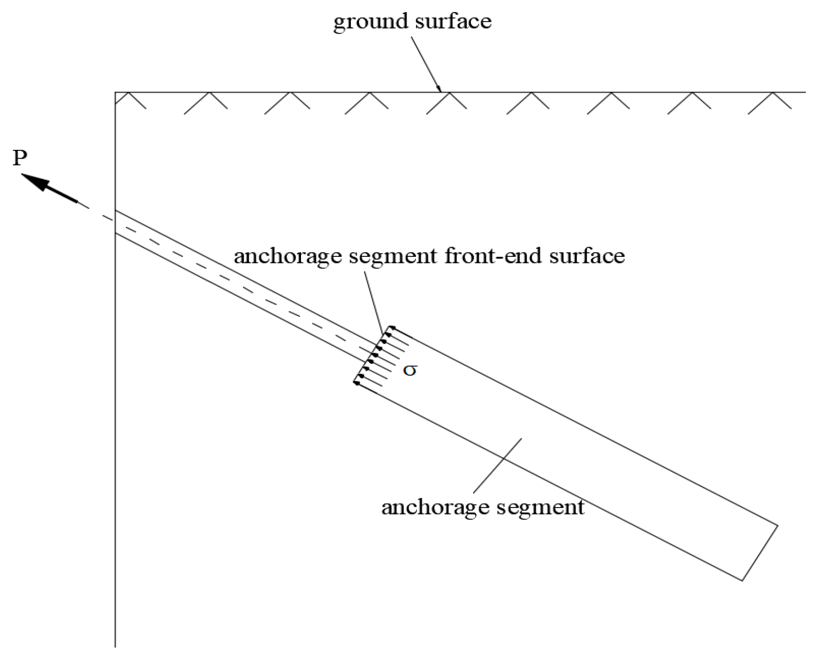
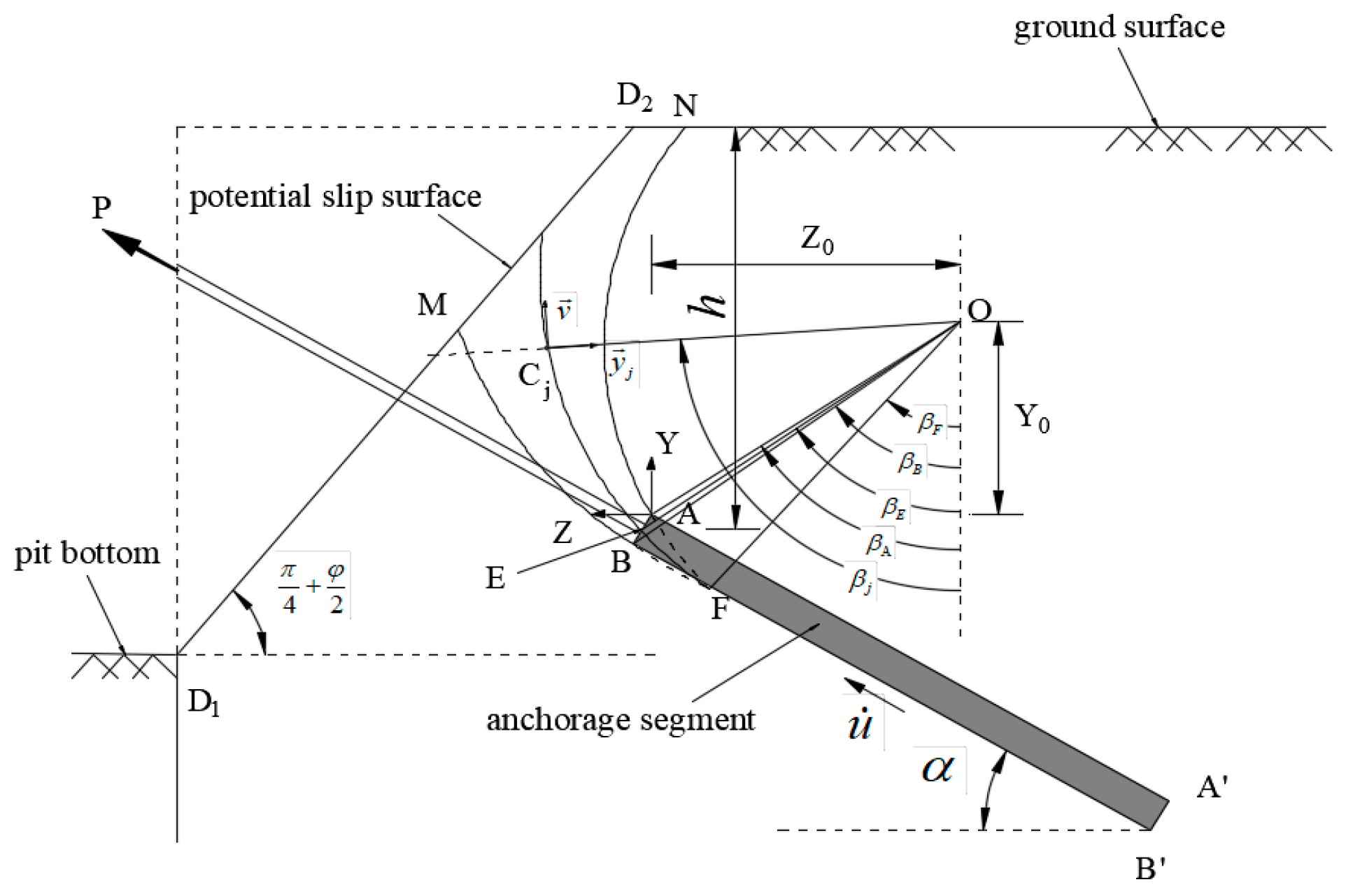
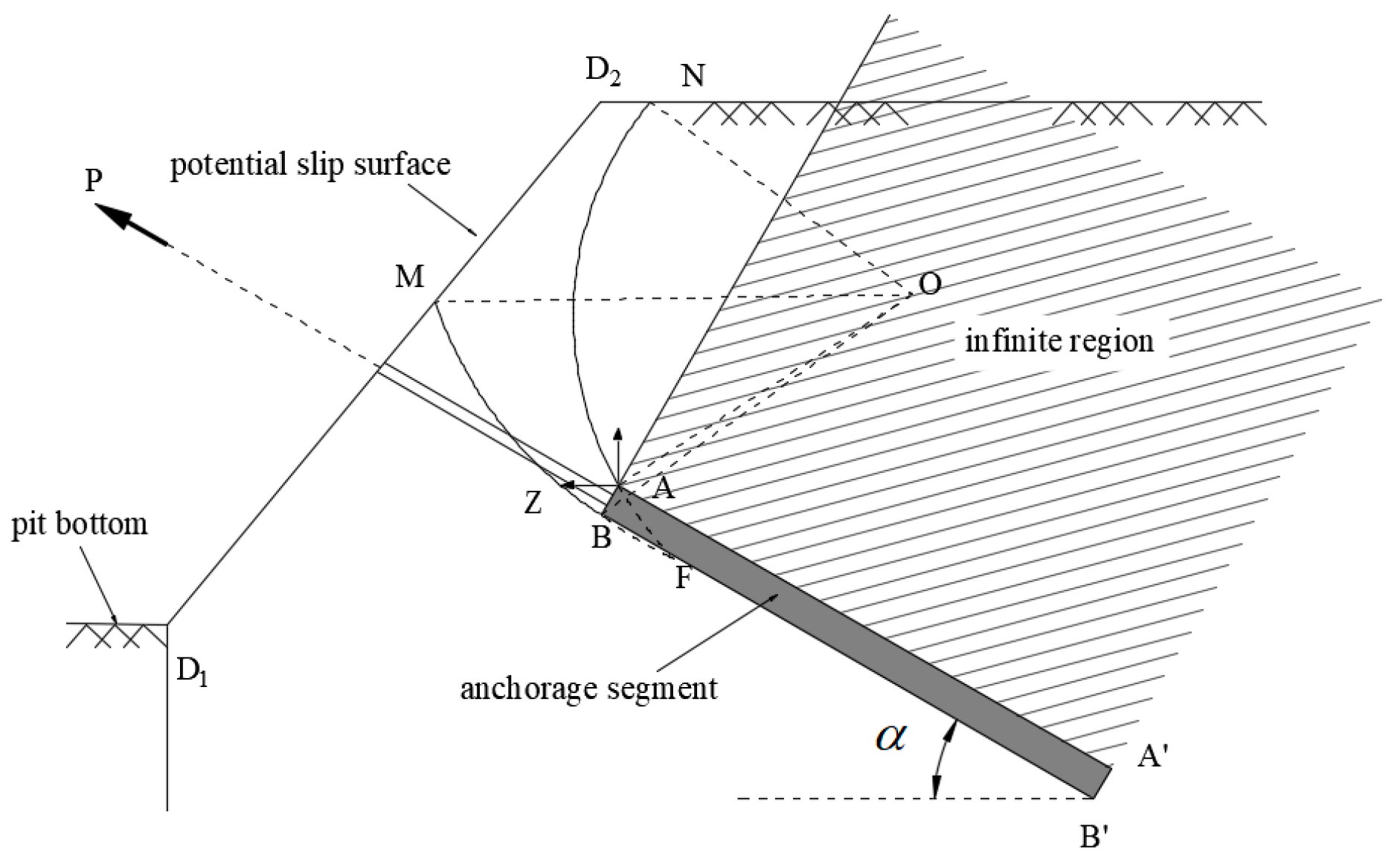
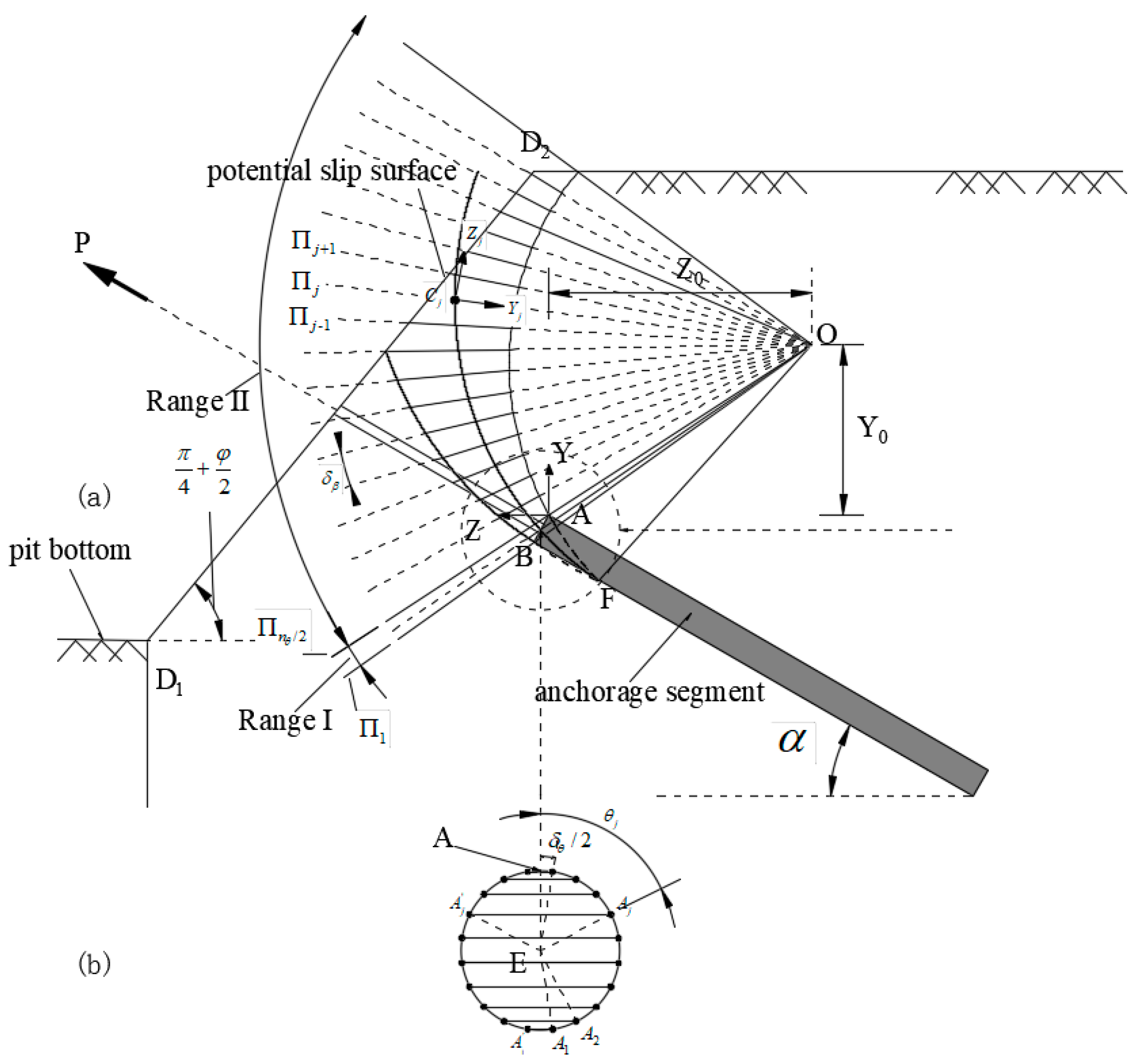
2. Construction of Failure Model

The structure of the expanded anchor cable studied in the present paper is shown in Figure 1. As shown in this figure, the cable’s structure could be divided into two parts (i.e., the free segment and the anchorage segment). The anchorage segment included two bearing bodies and a grouting body. In the present paper, the bearing body near the front-end surface of the anchorage segment and that near the back-end surface are referred to as the first and second bearing bodies, respectively. Each bearing body was anchored with two steel strands that were symmetrically located on both sides of the vertical plane crossing the longitudinal axis of the anchorage segment cylinder. The bearing bodies were firmly linked to the surrounding grouting body to ensure that the pullout force was transmitted to the surrounding soil through the anchorage body. To allow the steel strands to freely deform, isolating pipes were placed outside the steel strands. The pullout capacity provided by the free segment of an anchor cable is much smaller than that of the anchorage segment; hence, it was neglected in the present study. When constructing the failure model of the expanded anchor cable, its individual structures (i.e., bearing bodies and steel strands) were ignored. However, these were taken into account in the numerical simulations presented in the later sections.

It should be noted that we only studied the ultimate pullout capacity of a single expanded anchor cable arranged in a homogeneous soil stratum. We assumed that: (1) the soil was an ideal elastic–plastic material, obeying the Mohr–Coulomb yield criterion and complying with the associated flow rule when yielding; (2) the potential slip surface in the soil area outside the pit was generated due to the construction of the foundation pit and followed Rankine’s active earth pressure theory. It was necessary for the anchorage segment to be buried below the potential slip surface in order to obtain the pullout capacity. Thus, the resistance provided by the soil above the potential slip surface was not considered.

The calculated pullout capacity of the expanded anchor cable consisted of the later resistance and the end resistance, as the pullout capacity provided by the free segment was neglected in the present study. Corresponding to these two forces, the failure model of the expanded anchor cable was divided into two regions (i.e., the soil region at the front surface of the anchorage segment, and the anchorage segment and its surrounding soil, which is also referred to as the anchorage segment region). This is described in further detail in the following sections.

2.1. Failure Model of the Soil Region at the Front Surface of the Anchorage Segment

(1)

Failure mechanism

Under the end resistance of an expanded anchor cable, the strained condition of the soil located in the front-end surface of the anchorage segment (Figure 2) is similar to the condition of the soil in front of a shield tunnel face when the shield pressure is uniformly distributed on the tunnel face. Therefore, referring to the failure mechanism of the soil in a tunnel face [20,21], a three-dimensional logarithmic spiral failure model was adopted for the soil at the front surface of the anchorage segment. The soil region at the front surface of the anchorage segment could be renamed the logarithmic spiral region. To be specific, the logarithmic spiral region represents the soil zone at the front end of the anchorage segment, which is surrounded by three-dimensional logarithmic spirals.

Figure 3 shows the cross-sections of the failure model of the logarithmic spiral region in the vertical plane (YAZ) passing through the cable axis. As shown in Figure 3, the expanded anchor cable with a buried depth of h in a homogeneous stratum is destroyed under the action of pullout capacity P, the cross-section is bounded by two log spirals emerging from A and B with a common center O, the intersection of the side surface of the anchorage segment and the YAZ plane is AA’ and BB’, and D1D2 is the intersection of the potential slip surface and the YAZ plane.

(2)

Velocity field

The velocity field was considered in this study as follows: the logarithmic spiral region was damaged according to the above failure model under the action of pullout capacity P, leading to velocity discontinuity on the rupture surface or the so-called velocity discontinuity surface. Specifically, the logarithmic spiral region presented a three-dimensional rotation failure mechanism generated by rotation around the horizontal axis of point O with a uniform angular velocity $\omega$. Its velocity discontinuity surface intersected the symmetric plane at two logarithmic spirals, AN and BM, with a common rotation center O, as shown in Figure 3. In the YAZ plane, the possible region of the rotation center point O was the region formed by the intersection of the semi-infinite region on the right side of the straight line BA and above the straight line AA′, as shown in Figure 4.

The expressions of the logarithmic spirals AN and BM could be written as follows:

$$r_{AN}=r_A·\exp \left[\left({\beta }_A-\beta \right)·\tan \phi \right]$$

(1)

$$r_{BN}=r_B·\exp \left[\left(\beta -{\beta }_B\right)·\tan \phi \right]$$

(2)

where

$$r_A=\sqrt{Z_0^2+Y_0^2}$$

(3)

$$r_B=\sqrt{{(D_m\sin \alpha -Z_0)}^2+{(D_m\cos \alpha +Y_0)}^2}$$

(4)

$${\beta }_A=\arctan (-\frac{Z_0}{Y_0})$$

(5)

$${\beta }_B=\arctan (-\frac{D_m\sin \alpha -Z_0}{D_m\cos \alpha +Y_0})$$

(6)

In the above expressions, $r_A\mathrm{and} r_B$ are the lengths of OA and OB, respectively; ${\beta }_A$ and ${\beta }_B$ are the angles between the lines OA or OB and the vertical direction, respectively; φ is the internal friction angle of the soil stratum; and $Y_0$ and $Z_0$ are the Y-axis and Z-axis coordinates of the rotation center O in the cartesian coordinate system YAZ, respectively.

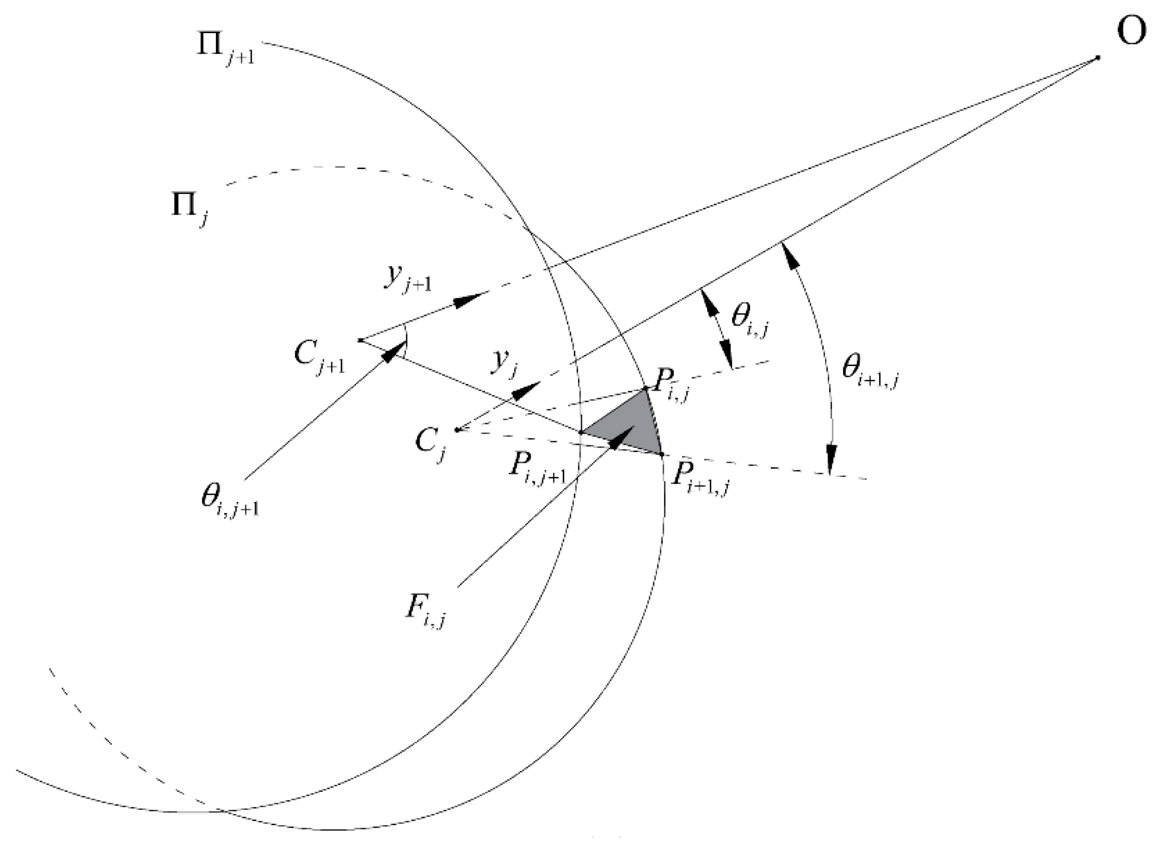
(3)

Geometrical construction of the 3D velocity discontinuity surface in logarithmic spiral region

The spatial discretization technique proposed in [20,21] was adopted to generate the 3D velocity discontinuity surface in the logarithmic spiral region. The basic principles were as follows: the failure model was discretized by several radial planes that all intersected at one point, and the intersection lines of the radial planes and velocity discontinuity surfaces were discretized into a series of points. The discrete points representing the contour of the failure model in any radial plane could be generated through those located in the previous radial plane according to the normality condition between the newly generated points and the points in the previous plane. Following this method, the contours of the failure model were successively generated; hence, the 3D velocity discontinuity surface was also generated.

As shown in Figure 5, each point $P_{i,j}$ of the velocity discontinuity surface was defined by an index $i$, representing the position of this point in a given plane, and an index $j$, corresponding to the plane in which this point was located. The method for the generation of the 3D surface involved computing the coordinates of any point $P_{i,j+1}$ of plane ${\prod }_{j+1}$ using the coordinates of two points, $P_{i,j}$ and $P_{i+1,j}$, in the previous plane ${\prod }_j$. The spatial discretization technique was applied in this paper, as shown in Figure 6. In this case, according to whether the plane passed through the front-end surface of the anchorage segment, the failure range could be divided into Range I or Range II, as shown in Figure 6a. Range I contained the radial plans that intersected with the front-end surface of the anchorage segment, and Range II contained the radial plans that did not intersect the front-end surface of the anchorage segment. In Range I, the generation of new points began with the use of points $A_1$ and $A_1^{\prime }$ of the front-end surface of the anchorage segment (Figure 6b). These two points belonged to plane ${\prod }_1$ and could be renamed $P_{i,1}$ and $P_{i+1,1}$. Then, the new point $P_{i,2}$, which belonged to plane ${\prod }_2$, could be generated by these two points. Similarly, the points $A_2$ and $A_2^{\prime }$, belonging to ${\prod }_2$, could be renamed $P_{i-1,2}$ and $P_{i+1,2}$. Therefore, two new points ($P_{i-1,3}$ and $P_{i,3}$) could be created by the three points $P_{i-1,2}$, $P_{i,2}$, and $P_{i+1,2}$. This operation was repeated until the end of Range I. In each plane ${\prod }_{j+1}$, j points were generated, with two other points located on the contour of the front-end surface of the anchorage segment already present. Thus, the total number of points in plane ${\prod }_{j+1}$ was j+2. In Range II, the contours were successively generated until the end of Range II, following the same method. Finally, the entire velocity discontinuity surface in the logarithmic spiral region was generated. For more details concerning the spatial discretization technique, the reader can refer to [20,21].

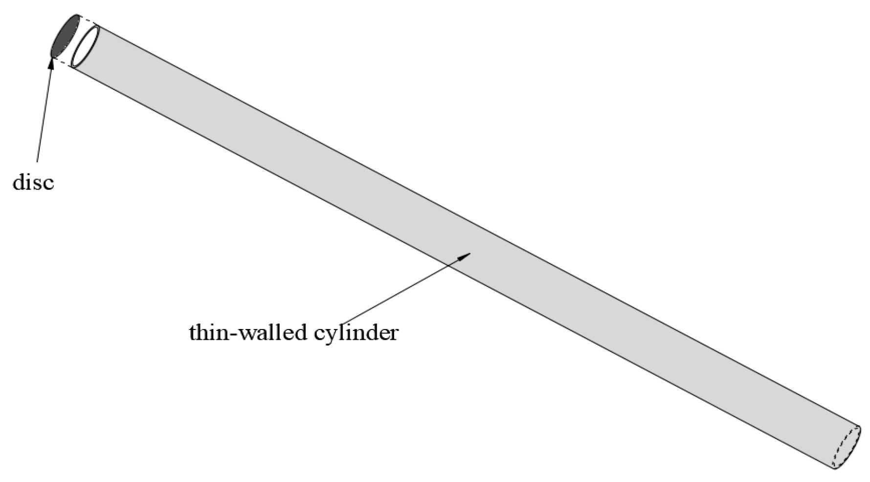
2.2. The Failure Model of the Anchorage Segment Region

(1)

Failure mechanism

When the failure limit of the anchorage segment region occurs, the interface between the anchorage segment and the soil presents shear failure, and its breakage mechanism was assumed to satisfy the slippage model [13].

(2)

Velocity field

The velocity field of the anchorage segment region is shown in Figure 7. The velocity discontinuity surface between the anchorage segment and the soil is referred to as the anchorage segment side surface, which presented as a cylindrical surface [13]. The narrow transition layer of the interface between the anchorage segment and its surrounding soil, which was bounded by two parallel surfaces (i.e., the anchorage side surface and the soil slip surface), was considered in the present study. The relative velocity along the axial direction of the rod body is $\dot{u}$. To satisfy the requirement of the dilatancy effect of Mohr–Coulomb materials on the relative velocity of the two sides of the velocity discontinuity surface, the separation velocity between the two sides of the velocity discontinuity surface should be $\dot{u}\tan \phi$ [22,23]. The front-end surface of the anchorage segment, located at the intersection of the logarithmic spiral region and the anchorage segment region, was assumed to be a disc with infinite stiffness, independent of the cylinder, as shown in Figure 8.

3. Upper-Bound Solution of Ultimate Pullout Capacity of Expanded Anchor Cable

The deduction of the upper-bound solution for the ultimate pullout capacity of the expanded anchor cable based on the upper-bound theorem of limit analysis is presented in this section. Because of the different velocity fields, the power of the logarithmic spiral region and the anchorage segment region were calculated separately; then, the end resistance and lateral resistance were obtained, followed by several algebraic operations. Finally, the ultimate pullout capacity could be computed by summing the end resistance and lateral resistance.

3.1. Calculation Theory of Upper-Bound Theorem of Limit Analysis

The upper-bound theorem of limit analysis was adopted to account for any failure mechanism with kinematic permission. Based on the virtual power theory, a reasonable upper-bound solution for the failure load of any failure model, which can be regarded as the upper limit of the actual ultimate load, can be obtained by equating the rate of work of the external force with the internal energy dissipation [24,25,26]. This reads as follows:

$${\int }_A{T}_i{\dot{u}}_i{}^{*}dA+{\int }_v{F}_i{\dot{u}}_i{}^{*}dv={\int }_A{\sigma }_{ij}{\dot{\epsilon }}_{ij}{}^{*}dv$$

(7)

where $T_i$ and $F_i$ are the surface traction and physical force, respectively; ${\sigma }_{ij}$ is the stress tensor; and ${\dot{u}}_i{}^{*}$ and ${\dot{\epsilon }}_{ij}{}^{*}$ are the virtual velocity and strain rate in the velocity field corresponding to the virtual failure model, respectively.

In this study, the external forces were the weight of the soil included in the failure model and the weight of the expanded anchor cable, and the only source of internal energy dissipation was the soil deformation that occurred along the velocity discontinuity surfaces. The power calculation was divided into two regions (i.e., the logarithmic spiral region and the anchorage segment region), according to the different velocity fields presented in Section 2; then, the lateral resistance and end resistance could be computed, respectively.

For each region, by equating the total rate of work carried out by the external forces with the total rate of internal energy dissipation on the velocity discontinuity surfaces, and by conducting several algebraic operations, the ultimate lateral resistance $P_1$ and ultimate end resistance $P_2$ were determined as follows:

$$P_1=\frac{W_1+W_{G1}}{\dot{u}}$$

(8)

$$P_2=\frac{{\dot{W}}_D+{\dot{W}}_{\gamma }}{\dot{u}}$$

(9)

where P denotes the ultimate pullout capacity; $\dot{u}$ denotes the axial velocity along the cable; $W_1$ denotes the rate of internal energy dissipation of the anchorage segment region; $W_{G1}$ denotes the rate of work carried out by the gravity of the anchorage segment; ${\dot{W}}_D$ denotes the rate of internal energy dissipation of the velocity discontinuity in the logarithmic spiral region; and ${\dot{W}}_{\gamma }$ denotes the rate of work carried out by the gravity of the soil in the logarithmic spiral region.

By summing $P_1$ and $P_2$, the ultimate pullout capacity of the expanded anchor cable could be obtained as follows:

$$P=P_1+P_2$$

(10)

3.2. Ultimate End Resistance Calculation

Through the power calculation of the logarithmic spiral region and several algebraic operations, the ultimate end resistance could be obtained (Equation (9)), and the final solution was determined through the particle swarm optimization (PSO) algorithm. The calculations are discussed in detail in this section.

3.2.1. Power Calculation of Logarithmic Spiral Region

In the logarithmic spiral region, through the calculation method of elementary surfaces and volumes generated by adjacent points [27], the elementary rates of work and rates of internal energy dissipation were obtained. Finally, the computation of the rate of work was achieved by the summation of the elementary rates of work, and the calculation of the internal energy dissipation was carried out by the summation of the elementary energy dissipations along the different elementary surfaces. The rate of work of the soil weight and the rate of internal energy dissipation of the velocity discontinuity surfaces in the logarithmic spiral region could be finally calculated as follows [20]:

$$\begin{array}{ll}{\dot{W}}_{\gamma }& ={\displaystyle {\iiint }_V\overrightarrow{\gamma }\cdot \overrightarrow{v}dV=\underset{i,j}{\Sigma }}(\overrightarrow{\gamma }\cdot {\overrightarrow{v}}_{i,j}\cdot V_{i,j}+\overrightarrow{\gamma }\cdot {\overrightarrow{v}}_{{}_{i,j}}^{\prime }\cdot V_{{}_{i,j}}^{\prime })\\ & =\omega \gamma \underset{i,j}{\Sigma }(R_{i,j}{V}_{i,j}\sin {\beta }_{i,j}+R_{{}_{i,j}}^{\prime }{V}_{{}_{i,j}}^{\prime }\sin {\beta }_{{}_{i,j}}^{\prime })\end{array}$$

(11)

$$\begin{array}{ll}{\dot{W}}_D& ={\displaystyle {\iint }_{S}cv\cos \phi dS=}\underset{i,j}{\Sigma }(c{v}_{i,j}{S}_{i,j}\cos \phi +c{v}_{{}_{i,j}}^{\prime }{S}_{{}_{i,j}}^{\prime }\cos \phi )\\ & =\omega c\cos \phi \underset{i,j}{\Sigma }(R_{i,j}{S}_{i,j}+R_{{}_{i,j}}^{\prime }{S}_{{}_{i,j}}^{\prime })\end{array}$$

(12)

In contrast to the blow-out failure mechanism of the shield tunnel face described in [20], which presented only one type of failure model wherein the velocity discontinuity surfaces all intersected with the ground surface, two typical failure models for the logarithmic spiral region are shown in Figure 8 because the coordinates of the rotation center point O differed, and the potential slip surface was also considered. In the first model, the boundary lines AN and BM of the velocity discontinuity surface in the vertical plane intersect with the ground surface at point N and with the potential slip surface at point M, respectively (Figure 9a); in the second model, the logarithmic spirals AN and BM both intersect with the potential slip surface (Figure 9b).

3.2.2. Determination of Minimum Upper-Bound Solution of End Resistance

The upper-bound solution of the ultimate end resistance was determined by the coordinates of the rotation center point O. It was necessary to decide the coordinates of point O that could minimize the possible upper-bound solution in order to obtain the real upper-bound solution for the ultimate end resistance. In the present study, the particle swarm optimization (PSO) algorithm [28,29] was adopted to identify the optimal upper-bound solution for the ultimate end resistance of the expanded anchor cable and determine the corresponding failure model under the determined ultimate end resistance.

The application of the particle swarm optimization algorithm was as follows: (1) each particle represented the coordinates of the rotation center O, denoted $x_i{}^j(Y_i{}^j,Z_i{}^j)$, with index i representing the number of particles and index j representing the number of iterations; (2) each particle’s fitness, which was represented by the ultimate end resistance corresponding to the rotation center $x_i{}^j(Y_i{}^j,Z_i{}^j)$, could be calculated according to Equation (9). For the initial population number N, each particle had an initial position $x_1{}^0,x_2{}^0,\cdot \cdot \cdot ,x_N{}^0$ and an initial velocity $v_1{}^0,v_2{}^0,\cdot \cdot \cdot ,v_N{}^0$. The particle fitness values calculated from all the initial positions were regarded as the individual optimal solutions $p_1{}^0,p_2{}^0,\cdot \cdot \cdot ,p_N{}^0$, and the minimum value of all the individual optimal solutions was taken as the group optimal solution $p_g{}^0$. In the second step of the iteration, the particle velocity and position were updated according to Equations (13) and (14), respectively, and then the individual optimal solutions $p_1{}^1,p_2{}^1,\cdot \cdot \cdot ,p_N{}^1$ and the group optimal solution $p_g{}^1$ could be obtained following the same method. This process was repeated until G iterations had been completed, and the individual optimal solutions $p_1{}^G,p_2{}^G,\cdot \cdot \cdot ,p_N{}^G$ and group optimal solution $p_{\mathrm{g}}{}^G$ could be obtained. In each iteration, the optimal solution (i.e., minimum upper-bound solution for the end resistance) needed to be compared with the group optimal solution. If the optimal solution was greater than the group optimal solution, the optimal solution was updated with the current group optimal solution. To be specific, in the first iteration, the optimal solution was equal to $p_{\mathrm{g}}{}^0$; after G iterations, the optimal solution was the minimum of $p_g{}^1,p_g{}^2,\cdot \cdot \cdot ,p_g{}^G$. In order to ensure the accuracy of the calculation results, the population number and the number of iterations were determined through a corresponding convergence analysis:

$$v_i^j=w{v}_i^{j-1}+c_1{r}_1(p_i^{j-1}-x_i^{j-1})+c_2{r}_2(p{g}^{j-1}-x_i^{j-1})$$

(13)

$$x_i^j=x_i^{j-1}+v_i^j$$

(14)

where w is the weighting factor; $c_1$ and $c_2$ are the individual learning factor and group learning factor, respectively; and $r_1$ and $r_2$ are two random numbers with a value in the range [0, 1], which were introduced to increase the computation randomness.

3.3. Ultimate Lateral Resistance Calculation

Through the power calculation of the anchorage segment region and several algebraic operations, the ultimate lateral resistance could be obtained (Equation (8)). In the anchorage segment region, the source of internal energy dissipation was the expansion deformation of the soil and the relative motion between the anchorage segment and its surrounding soil, and the rate of work was attributed to the gravity of the anchorage segment. The calculations are discussed in detail in this section.

(1)

Rate of internal energy dissipation of the anchorage segment region

The rate of internal energy dissipation depended on the soil expansion deformation, which could be computed as follows:

$${\dot{W}}_{\epsilon }=T\dot{\mathrm{u}}\tan \phi$$

(15)

where $T$ is the resultant force of the normal pressure acting on the side surface of the anchorage segment; $\dot{u}$ is the axial velocity along the cable; and $\phi$ is the internal friction angle of the contact surface between the anchorage segment and its surrounding soil, which could be taken as approximately equal to that of the surrounding soil.

As depicted in Figure 10, the resultant normal force T could be decomposed into two parts: the resultant normal pressure generated by the vertical component of the soil pressure, denoted as Q herein, and the force generated by the horizontal component of the soil pressure, denoted as P herein.

Thus, the vertical component of the soil pressure $q_v$ could be written as:

$$q_v=\gamma [h-R_m\cos \theta \cos \alpha +L_m\sin \alpha ]$$

(16)

Then, the differential of Q, which denoted the resultant normal pressure corresponding to an infinitesimal area $\mathrm{d}A$, could be computed through the following equation:

$$\begin{array}{ll}dQ& =q_{v}R\mathrm{d}\theta \cos \theta \cos \theta \mathrm{d}L\cos \alpha \cos \alpha \\ & =q_{v}R{\cos }^2\theta {\cos }^2\alpha \mathrm{d}\theta \mathrm{d}L\end{array}$$

(17)

Finally, Q could be obtained through the integral of $\mathrm{d}Q$ over the side surface of the anchorage segment:

$$\begin{array}{ll}Q& ={\displaystyle {\iint }_{\Sigma }\mathrm{d}Q}\\ & =4{\displaystyle {\int }_0^{\frac{\pi }{2}}{\displaystyle {\int }_0^{L_m}{q}_v{R}_m{\cos }^2\theta {\cos }^2\alpha \mathrm{d}L\mathrm{d}\theta }}\\ & =\frac{L_m{R}_m\gamma {\cos }^2\alpha (6\pi h-16R_m\cos \alpha +3\pi L_m\sin (\alpha ))}{6}\end{array}$$

(18)

Similarly, the horizontal component of the soil pressure $q_h$, $\mathrm{d}P$, and P could be computed as follows:

$$q_h=K_0\gamma [h-R_m\cos \theta \cos \alpha +L_m\sin \alpha ]$$

(19)

$$\mathrm{d}P=q_h{R}_m\mathrm{d}\theta \sin \theta \sin \theta \mathrm{d}L=q_v{R}_m{\sin }^2\theta \mathrm{d}\theta \mathrm{d}L$$

(20)

$$\begin{array}{ll}P& ={\displaystyle {\int }_0^{2\pi }{\displaystyle {\int }_0^{L_m}{q}_h{R}_m{\sin }^2\theta \mathrm{d}L\mathrm{d}\theta }}\\ & ={\displaystyle {\int }_0^{2\pi }{\displaystyle {\int }_0^{L_m}{K}_0\gamma [h-R_m\cos \theta \cos \alpha }}+L\sin (\alpha )]R_m{\sin }^2\theta \mathrm{d}L\mathrm{d}\theta \\ & =\frac{K_0{L}_m{R}_m\gamma \pi (2h+L_m\sin \alpha )}{2}\end{array}$$

(21)

where $K_0$ is the lateral pressure coefficient, which could be taken as $K_0=1-\sin \phi$.

By summing Q and P, the total normal force T could be obtained. According to Equations (18) and (21), T could be expressed as:

$$\begin{array}{ll}T& =Q+P\\ & =\frac{L_m{R}_m\gamma {\cos }^2\alpha }{6}[6\pi h-16R_m\cos \alpha +3\pi L_m\sin (\alpha )]\\ & +\frac{K_0{L}_m{R}_m\gamma \pi (2h+L_m\sin \alpha )}{2}\end{array}$$

(22)

Hence, the internal energy dissipation caused by the soil expansion deformation could be computed as:

$$\begin{array}{ll}{\dot{W}}_{\epsilon }& =T\dot{\mathrm{u}}\tan \phi \\ & =\left\{\frac{L_m{R}_m\gamma {\cos }^2\alpha }{6}\right.[6\pi h-16R_m\cos \alpha +3\pi L_m\sin (\alpha )]\\ & +\left.\frac{K_0{L}_m{R}_m\gamma \pi (2h+L_m\sin \alpha )}{2}\right\}\dot{u}\tan \phi \end{array}$$

(23)

where $\gamma$ is the unit weight of the soil. All the other variables in Equations (16)–(23) can be easily identified from Figure 10.

The rate of internal energy dissipation was caused by the relative motion on the narrow transition layer of the interface between the anchorage segment and its surrounding soil. The velocity field on the narrow transition layer can be seen in Figure 7. In the transition layer, the rate of the internal energy dissipation per unit volume could be written as follows:

$$\dot{D}=(\tau \dot{\gamma }-\sigma \dot{\epsilon })t=c\dot{u}$$

(24)

where $\tau$ is the shearing stress; $\sigma$ is the normal stress; $t$ is the thickness of the narrow transition layer; $c$ is the cohesion of the soil; and $\dot{\epsilon }$ and $\dot{\gamma }$ denote the normal strain rate and shear strain rate, respectively. The latter could be written as:

$$\dot{\epsilon }=\frac{\dot{u}}{t}\tan \phi$$

(25)

$$\dot{\gamma }=\frac{\dot{u}}{t}$$

(26)

The summation of the rate of internal energy dissipation over the anchorage side surface was calculated by:

$${\dot{W}}_{D1}=\dot{D}\pi D_m{L}_m=\pi c{D}_m{L}_m\dot{u}$$

(27)

where $D_m$ denotes the anchorage segment diameter, and $L_m$ denotes the anchorage segment length.

The rate of the internal energy dissipation of the anchorage segment could be computed as follows:

$$\begin{array}{ll}{W}_1& ={\dot{W}}_{\epsilon }+{\dot{W}}_{D1}\\ & =\left\{\frac{L_m{R}_m\gamma {\cos }^2\alpha }{6}\right.[6\pi h-16R_m\cos \alpha +3\pi L_m\sin (\alpha )]\\ & +\left.\frac{K_0{L}_m{R}_m\gamma \pi (2h+L_m\sin \alpha )}{2}\right\}\dot{u}\tan \phi +\pi c{D}_m{L}_m\dot{u}\end{array}$$

(28)

(2)

Rate of work of anchorage segment weight

$$W_{G1}={\gamma }_m\pi {(\frac{D_m}{2})}^2{L}_m\dot{u}\sin \alpha$$

(29)

where ${\gamma }_m$ is the unit weight of the anchorage segment.

4. Example Analysis and Solution Validation

4.1. Theoretical Solution

In order to compare the theoretical results with the subsequent numerical simulation results, the three cases shown in

Table 1. Control parameters of expanded anchor cable.

Case	Anchorage Segment Length (m)	Free Segment Length (m)	Anchorage Segment Diameter (m)	Inclination Angle of Anchor Cable (°)	Stratum Friction Angle (°)	Buried Depth (m)
M1	10	9	0.6	30	10.6	7
M2	12	9	0.6	30	10.6	7
M3	10	9	0.6	45	10.6	7

were considered herein. It should be emphasized here that the inclination angle of the anchor cable represents the angle of the cable axis relative to the horizontal ground surface (i.e., $\alpha$ shown in Figure 2). The material properties of the soil used for this study were as follows: the density was 1770 kg/m³, the elastic modulus was 13.5 MPa, the shear modulus was 5 MPa, the friction angle was 10.6°, and the cohesion was 8 kPa.

The particle swarm optimization algorithm was used to obtain the optimal solution, which produced the optimal upper-bound solution for the end resistance (i.e., Equation (9)).

Table 2. Theoretical solutions.

Case	Lateral Resistance P1 (kN)	End Resistance P2 (kN)	Ultimate Pullout Force P (kN)
M1	610.1	217.4	861.7
M2	761.5	217.4	1019.3
M3	580.8	144.9	782.9

presents the calculation results. In this table, the lateral resistance was obtained by Equation (8), and the ultimate pullout capacity was computed by summing the end resistance and lateral resistance.

Only case M3 is presented here as an example, to limit the length of the manuscript. In this case, the values of the calculation parameters in the particle swarm optimization algorithm were as follows: $w =0.8$, $c_1=c_2=0.5$, and $r_1$ and $r_2$ were random variables between 0 and 1. Figure 11 presents the relationship between the optimal solutions (i.e., the ultimate end resistance) and the number of iterations calculated by the particle swarm optimization algorithm in the case M3. It can be seen that when the population number was $N=50$ and the number of iterations was $G=80$, the calculation approached a convergence state. Thus, the best solution value for the ultimate end resistance was about 144.9 kN.

The critical failure model for the logarithmic spiral region obtained from the spatial discretization technique is presented in Figure 12 for the case M3, with the help of MATLAB software. The 3D velocity discontinuity surfaces all intersected with the potential slip surface.

4.2. Numerical Solution

In order to verify the accuracy of the theoretical solution, the finite difference software FLAC3D was adopted to calculate the magnitude of the ultimate pullout capacity of an expanded anchor cable, and the results were compared with the theoretical upper-bound solution.

Corresponding to the theoretical analysis in the above sections, only the ultimate pullout capacity of a single expanded anchor cable arranged in a homogeneous soil stratum was analyzed in the numerical simulations. The three-dimensional numerical model was established according to the conditions of the expanded anchor cable considered in this paper (Figure 1), as shown in Figure 13. In this Figure, the parameters of the anchor cable accorded with those of case M1 listed in Table 1. In addition, the two bearing bodies had the same length of 0.5 m (Figure 14). In order to ensure the simulation accuracy, the length, width, and height of the numerical model were 22.4 m, 20 m, and 17.0 m, respectively (as shown in Figure 13). The boundary conditions were set to normal constraints for all four vertical model planes, and the displacements at the bottom of the model were fixed. On the excavation side of the foundation pit, normal constraints were applied below the bottom of the pit. In the model, 3D grids were used to model the soil, the steel strand, the bearing body, and the grouting body of the anchorage segment. The steel strand and bearing body adopted an elastic constitutive model, and the other 3D grids adopted the Mohr–Coulomb constitutive model. The calculation parameters of the soil and anchor cable are shown in

Table 3. Calculation parameter values.

Material	Density (kg/m3)	Elastic Modulus (MPa)	Shear Modulus (MPa)	Friction Angle (°)	Cohesion (kPa)
Steel strand	7800	200,000	77,000	-	-
Soil	1770	13.5	5	10.6	8.0
Bearing body	7000	22,000	9361.70	-	-
Grouting body	2200	21,897	9317.87	50.2	1960

.

Contact interfaces were established between the grouting body and the soil, the steel strand and the grouting body, and the steel strand and the bearing body to model the mechanical characteristics of the interfaces between the different structures. The normal stiffness and tangential stiffness of these interfaces were 10 times the equivalent stiffness of the soil element, and the cohesion and friction angle of the interface between the grouting body and its surrounding soil were taken as those of the adjacent soil [30]. In addition, the values of the cohesion and friction angle of the contact surface between the steel strand and the bearing body were set large enough to ensure that they were firmly connected, while those between the steel strand and the grouting body were set to zero to simulate the effect of isolating pipes outside the steel strand. The pullout capacity provided by the free segment of the anchor cable was much smaller than that of the anchorage segment; hence, it was neglected in the model. Thus, the cohesion and friction angle of the contact surface between the grouting body and the surrounding soil were also taken as 0 in the free segment.

In the numerical simulation, the pullout process of the expanded anchor cable was simulated by applying the pullout force gradually from a small magnitude to a large magnitude that was uniformly taken on by the four steel strands. The ultimate pullout capacity was determined according to the following computation convergence characteristics: the pullout stage at which the computation stopped converging was first determined, and then the pullout force in the previous pullout stage could be considered as the ultimate pullout capacity.

Figure 15 depicts the relationship between the pullout force P and the slipping displacement S of the anchorage segment in case M1. As can be seen in Figure 15, when the pullout force applied to the steel strands was small, the displacement of the anchorage segment was small; when the applied pullout force was close to the ultimate pullout capacity, the anchorage segment presented significant slip; indeed, when the pullout force exceeded the ultimate pullout capacity, the slipping displacement of the anchorage segment could not achieve a convergence state. To be specific, when the pullout force was less than 750 kN, the slipping displacement was small; when reaching 750 kN, the slipping displacement of the anchorage segment was only 42.9 mm; when the pulling force continued to increase and reached the ultimate pullout capacity of 800 kN, a large slip with a magnitude of 570 mm occurred in the anchorage segment, but the anchor-cable–soil system could still approach an equilibrium state; when the pullout force reached 850 kN, the computation could not approach a convergence state. Thus, it could be concluded that the ultimate pullout capacity of the expanded anchor cable was 800 kN.

4.3. Solution Validation

The theoretical calculation and numerical simulation results of the three considered cases are summarized in

Table 4. Comparison between ultimate pullout capacity according to numerical and theoretical solutions.

Case	Lateral Resistance P1 (kN)			End Resistance P2 (kN)			Ultimate Pullout Capacity P (kN)
	Numerical	Theoretical	Error (%)	Numerical	Theoretical	Error (%)	Numerical	Theoretical	Error (%)
M1	575.5	610.1	6.0	176.5	217.4	23.2	800	861.7	7.71
M2	724.6	761.5	5.1	170.8	217.4	27.3	950	1019.3	7.29
M3	608.9	580.8	4.6	146.7	144.9	1.2	830	782.9	5.67

. It should be noted that in the numerical simulation, the lateral resistance $P_1$ and end resistance $P_2$ were all obtained through the Fish programming language embedded in FLAC3D. The results showed that the error between the numerical solution and the theoretical solution for the lateral resistance in the three cases was only 6.0%, whereas that for the end resistance was relatively large; however, it was still within 30%, and so the maximum error of the ultimate pullout capacity was 7.7%. This indicated that the proposed theoretical model demonstrated high reliability in the analysis of the ultimate pullout capacity of the expanded anchor cable.

In order to further illustrate the reliability and superiority of the present calculation method, the theoretical formula for the ultimate pullout capacity of an expanded anchor cable described in [18] was used for calculation, and the results were compared and discussed.

Zeng et al. [18] proposed an algorithm for the ultimate pullout capacity of an expanded anchor cable that could be divided into three parts, as follows:

$$T=T_1+T_2+T_3$$

(30)

where $T$ denotes the ultimate pullout capacity (i.e., $P$); $T_1$ denotes the ultimate lateral resistance of the free segment, which was neglected in the present paper; $T_2$ denotes the ultimate lateral resistance of the anchorage segment (i.e., $P_1$); and $T_3$ denotes the ultimate end resistance (i.e., $P_2$). $T_2$ and $T_3$ are given by:

$$T_2=\pi D_2{L}_2{\tau }_{fd}$$

(31)

$$T_3=\frac{\pi }{4}(D_2^2-D_1^2)P_D$$

(32)

All the variables in Equations (31) and (32) are identified in [18]. The values of the variables were as follows: $D_1=0.2\mathrm{m}$, ${\tau }_{fd}=31\mathrm{kPa}$, $\xi =0.5K_a$, and the values for the other variables are provided in Section 4.1. The results of the three considered cases are summarized in

Table 5. Comparison between numerical solutions and theoretical solutions based on [18].

Case	Lateral Resistance P1 (kN)			End Resistance P2 (kN)			Ultimate Pullout Capacity P (kN)
	Numerical	Zeng [18]	Error (%)	Numerical	Zeng [18]	Error (%)	Numerical	Zeng [18]	Error (%)
M1	575.5	587.9	2.15	176.5	54.8	68.95	800	642.7	19.67
M2	724.6	705.4	2.64	170.8	54.8	67.92	950	760.2	19.97
M3	608.9	587.9	3.45	146.7	54.8	62.65	830	642.7	22.57

.

According to this table, the results showed that the error between the numerical solution and the theoretical solution based on [18] for the lateral resistance in the three cases was only 3.45%. However, the error for the end resistance was relatively large, resulting in a maximum error of 68.95%, which was mainly due to the high value of $\xi$, in the range of $(0.5~0.95)K_a$. Combined, the maximum error of the ultimate pullout capacity was 22.57%, which was significantly higher than the error between the numerical simulation and the theoretical solution proposed in this paper. Compared with the technique presented in [18], the calculation method for the ultimate pullout capacity of the expanded anchor cable proposed in this paper was more accurate and reasonable, and has high applicability in practical engineering.

5. Model Application

In this section, the proposed model was adopted to analyze the influence of the key parameters on the ultimate pullout capacity of the expanded anchor cable. The influence of each variable on the ultimate lateral resistance, end resistance, and pullout capacity was investigated, and the values of the other parameters were based on those of case M1. When the anchorage segment diameter changed from 0.4 m to 0.8 m with a spacing of 0.1 m, the anchorage segment length changed from 6 m to 14 m with a spacing of 2 m, the free segment length changed from 6 m to 14 m with a spacing of 2 m, the inclination angle of the anchor cable change from 10° to 50° with a spacing of 10°, and the buried depth of the anchor cable changed from 6 m to 10 m with a spacing of 1 m.

5.1. Effect of Anchorage Segment Diameter

Figure 16 presents the ultimate pullout capacity, lateral resistance, and end resistance variation curves according to changes in the anchorage segment diameter. From this figure, it can be seen that the lateral resistance, end resistance, and ultimate pullout capacity all increased linearly with the increase in the anchorage segment diameter. When the diameter increased from 0.4 m to 0.8 m, the lateral resistance increased from 407.9 kN to 811.2 kN by about 99%, the end resistance increased from 184.9 kN to 251.4 kN by about 40%, and the ultimate pullout capacity increased from 592.8 kN to 1062.6 kN by about 79%. This indicated that the change in the anchorage segment diameter had a greater influence on the lateral resistance than on the end resistance. This was because the change in the anchorage segment diameter had a greater influence on the side surface area than on the three-dimensional velocity discontinuity surfaces in the logarithmic spiral region.

5.2. Effect of Anchorage Segment Length

Figure 17 presents the ultimate pullout capacity, lateral resistance, and end resistance variation curves according to an increase in the anchorage segment length. As can be seen, the anchorage segment length had a great influence on the lateral resistance, while it had nearly no influence on the end resistance. To be specific, when the anchorage segment length increased from 6 m to 14 m, i.e., the anchorage segment length increased by 133%, the lateral resistance increased from 336.7 kN to 922.6 kN by about 174%. This was because the increase in the anchorage segment length brought about a sharp increase in the lateral surface and the average buried depth of the anchorage segment. This led to a sharp increase in the normal soil pressure acting on the anchorage segment, but did not have any influence on the three-dimensional velocity discontinuity surfaces in the logarithmic spiral region. Therefore, the change in the anchorage segment length only affected the lateral resistance of the expanded anchor cable.

5.3. Effect of the Inclination Angle of the Anchor Cable

Figure 18 presents the ultimate pullout capacity, lateral resistance, and end resistance variation curves according to an increase in the inclination angle of the anchor cable. It can be seen from this figure that initially, the lateral resistance gradually increased, before gradually decreasing with the increase in the inclination angle of the anchor cable, reaching a maximum of about 610.1 kN when the inclination angle was 30 degrees. However, in general, the change in the inclination angle had a relatively small impact on the ultimate lateral resistance. With the increase in the inclination angle of the anchor cable, the end resistance and ultimate pullout capacity decreased. Specifically, when the inclination angle increased from 10° to 50°, the end resistance and ultimate pullout capacity decreased from 290.6 kN to 120.1 kN by about 58.7% and from 872.5 kN to 684.4 kN by about 21.6%, respectively.

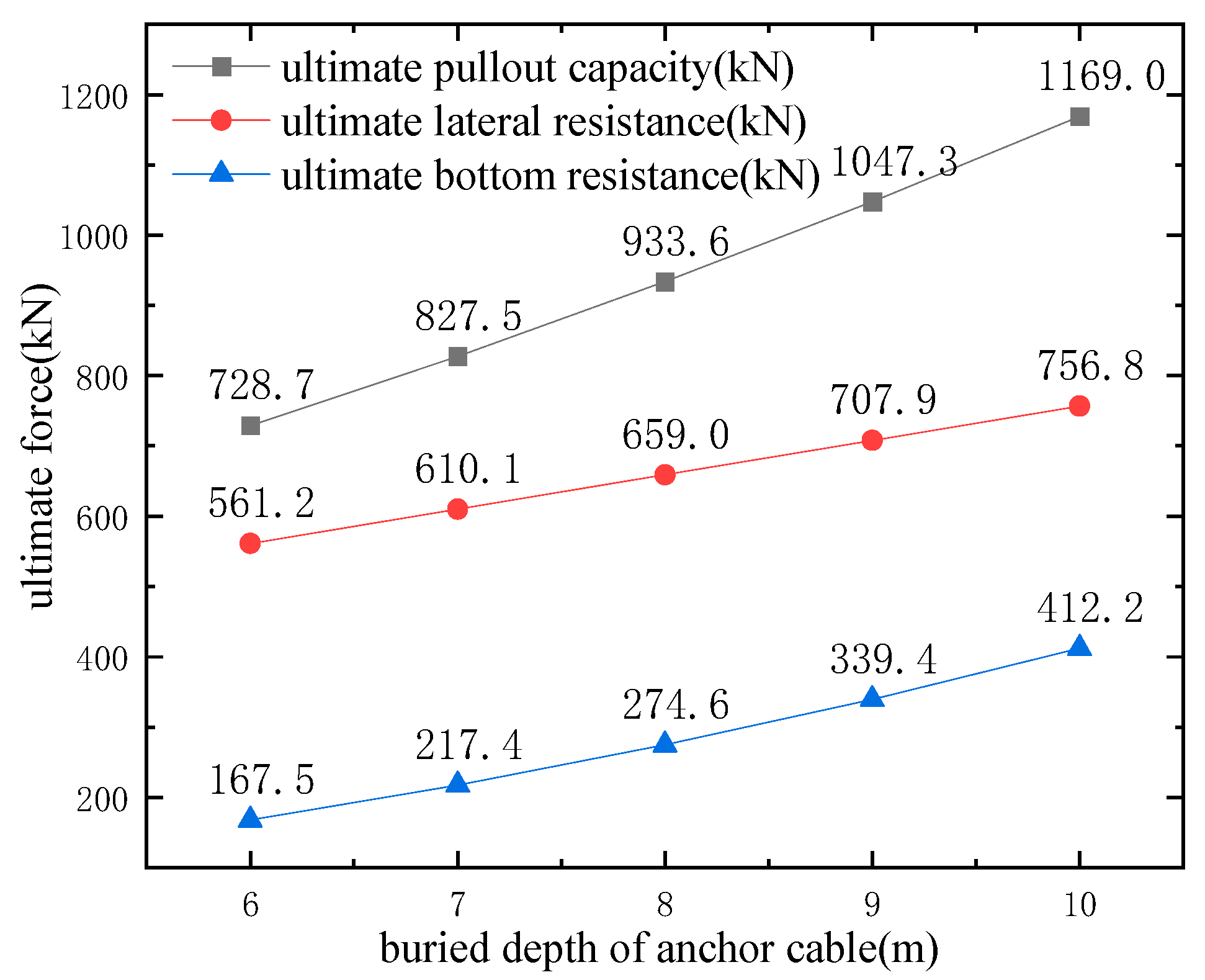
5.4. Effect of the Buried Depth of the Anchor Cable

Figure 19 presents the ultimate pullout capacity, lateral resistance, and end resistance variation curves according to the change in the buried depth of the anchor cable. The figure clearly shows that the lateral resistance, end resistance, and ultimate pullout capacity increased with the increase in the buried depth of the anchor cable. When the buried depth increased from 6 m to 10 m, the lateral resistance increased from 561.2 kN to 756.8 kN by about 35%, the end resistance increased from 167.5 kN to 412.2 kN by about 146%, and the ultimate pullout capacity increased from 728.7 kN to 1169.0 kN by about 60%.

6. Conclusions

A failure model based on the upper-bound theorem of limit analysis was presented in this paper. The expressions of the upper-bound solution for the ultimate lateral resistance and the ultimate end resistance were derived according to the principle of virtual power, and the final solution for the ultimate end resistance was determined by the particle swarm optimization algorithm. The upper-bound solution for the ultimate pullout capacity was obtained by summing the ultimate lateral resistance and ultimate end resistance. The accuracy of the proposed analytical solution was verified through a comparison with three-dimensional numerical simulations, which were calculated by the finite difference software FLAC3D. In addition, the superiority of the proposed analytical solution was well demonstrated through a comparison with an existing theoretical method. Regarding the application of the failure model, the influence of the anchor cable’s key parameters on the ultimate lateral resistance, end resistance, and ultimate pullout capacity was discussed in detail. The following conclusions could be drawn:

(1)

A failure model of an expanded anchor cable located in a homogeneous stratum was constructed. The logarithmic spiral failure model was used as the failure model of the soil region at the front surface of the anchorage segment, representing the first time that this model has been implemented to calculate the end resistance of an expanded anchor cable. The failure mechanism of the anchorage side surface was assumed to satisfy the slippage model. The expressions of the ultimate lateral resistance and ultimate end resistance could be derived, respectively, from the power calculations for the two models and several algebraic operations. Due to the particularity of the boundary conditions in this paper, the rotation center points of the logarithmic spiral lines were uncertain. Therefore, the particle swarm optimization algorithm was used to determine the optimal solution of the end resistance.

(2)

The theoretical calculation results were compared with the numerical simulation in three cases. The results showed that the error between the numerical solution and the theoretical solution for the lateral resistance in the three cases was only 6.0%; however, the error for the end resistance was relatively large, though still within 30%, and so the maximum error for the ultimate pullout capacity was 7.7%. These errors were much smaller than the errors between the numerical simulation and the theoretical calculation method proposed in [18] for the same cases. This indicated that the proposed theoretical model had high reliability and superiority in the analysis of the ultimate pullout capacity of the expanded anchor cable.

(3)

The ultimate lateral resistance and total ultimate pullout capacity increased significantly with the increase in the anchorage segment diameter, anchorage segment length, and buried depth of the expanded anchor cable. The ultimate end resistance increased significantly with the buried depth, increased slightly with the anchorage segment diameter, and was almost unaffected by the anchorage segment length.

(4)

With the increase in the inclination angle of the anchor cable, the end resistance and the ultimate pullout capacity gradually decreased, while the lateral resistance increased first and then decreased. However, in general, the change in the inclination angle of the anchor cable had a relatively small effect on the ultimate lateral resistance.

References

- Qian, Q.; Chen, X. Fully Developing and Utilizing Underground Space to Construct Resource-saving and Environment-friendly City. Chin. Civil Air Defence. 2007, 9, 15–18. [Google Scholar]
- Sun, Y.S.; Li, Z.M. Analysis of Deep Foundation Pit Pile-Anchor Supporting System Based on FLAC3D. Geofluids 2022, 2022, 1699292. [Google Scholar] [CrossRef]
- Fujita, K. A method to predict the load-displacement relationship of ground anchors. In Proceeding of the 9th International Conference on Soil Mechanics and Foundation Engineering; The Japanese Society of Soil: Tokyo, Japan, 1977; pp. 58–62. [Google Scholar]
- Barley, A.D.; Hossain, D.; Liao, H.J.; Hsu, S.T. Should grouted anchors have short tendon bond Length? J. Geotech. Geoenvironmental Eng. 1999, 125, 808–812. [Google Scholar] [CrossRef]
- Peng, H.; Xiao, X.Q.; Dong, Z.Y. Study on Deformation Influence of Deep Foundation Pit Pile-anchor Supporting System Nearby Metro Structure. Appl. Mech. Mater. 2014, 638–640, 1190–1194. [Google Scholar] [CrossRef]
- Liu, Z.; Guo, G. Application of innovation underreamed ground anchorage with capsule. In Proceedings of the International Conference Organized by the Deep Foundations Institute, Melbourne, Australia, 4–7 December 2017; pp. 310–319. [Google Scholar]
- Lin, G.; Zhang, L.; Wen, Z. Numerical Simulation on Expanded Anchor rod Supporting System for Deep Foundation Pit. Subgrade Eng. 2015, 92–98+111. [Google Scholar] [CrossRef]
- Evans, T.M.; Nan, Z. Three-Dimensional Simulations of Plate Anchor Pullout in Granular Materials. Int. J. Geomech. 2019, 19. [Google Scholar] [CrossRef]
- Hsu, S.T.; Wang, C.C.; Wu, S.; Tung, H.C. Computer simulation on the uplift behavior of an arrayed under-reamed anchor group in dense sand. In Proceedings of the International Conference on Systems and Informatics, Hangzhou, China, 11–13 November 2017; pp. 546–551. [Google Scholar]
- Hsu, S.T. A numerical study on the uplift behavior of underreamed anchors in silty sand. Adv. Mater. Res. 2011, 189–193, 2013–2018. [Google Scholar] [CrossRef]
- Serrano, A.; Olalla, C.; Gonzalez, J. Ultimate bearing capacity of rock masses based on the modified Hoek-Brown criterion. Int. J. Rock Mech. Min. Sci. 2000, 37, 1013–1018. [Google Scholar] [CrossRef]
- Liu, B.; Zhang, G.; Yang, W.; Ren, X.; Song, C. Mechanical Characters of Bit Expanded Anchor Rods in Saturated Fine Sand Stratum. Chin. J. Undergr. Space Eng. 2016, 12, 412–419. [Google Scholar]
- Wang, Z.; Wang, Q.-k.; Ma, S.-j.; Xue, Y.; Xu, S.-f. A method for calculating ultimate pullout force of recoverable under-reamed prestressed anchor cable. Rock Soil Mech. 2018, 39, 202–208. [Google Scholar]
- Ma, H.-C.; Tan, X.-H.; Qian, J.-Z.; Hou, X.-L. Theoretical analysis of anchorage mechanism for rock bolt including local stripping bolt. Int. J. Rock Mech. Min. Sci. 2019, 122, 104080. [Google Scholar] [CrossRef]
- Gang, G.; Zhong, L.; Aiping, T.; Yibing, D.; Jiqiang, Z.; Roman, W.-W. Model Test Research on Bearing Mechanism of Underreamed Ground Anchor in Sand. Math. Probl. Eng. 2018, 2018, 9746438. [Google Scholar]
- Guo, G.; Yang, D.; Zhong, G.; Xue, Z.Z. Test and design method for the performance of anchor nodes between an underreamed anti-floating anchor and the bottom structure. Environ. Earth Sci. 2019, 371, 022079. [Google Scholar] [CrossRef]
- Zhang, J.; Jiang, Z. On-field Testing Bearing and Deformation Characteristics of Underreamed Compression Anchors. Chin. J. Undergr. Space Eng. 2018, 14, 554–558. [Google Scholar]
- Zeng, Q.-y.; Yang, X.-y.; Yang, C.-y. Mechanical mechanism and calculation method of bit expanded anchor rods. Rock Soil Mech. 2010, 31, 1359–1367. [Google Scholar]
- Liang, Y. Study on Anchoring Mechanism of Under-Reammed Pressive Ground Anchor; China Academy of Railway Sciences: Beijing, China, 2012. [Google Scholar]
- Mollon, G.; Dias, D.; Soubra, A.-H. Rotational failure mechanisms for the face stability analysis of tunnels driven by a pressurized shield. Int. J. Numer. Anal. Methods Geomech. 2011, 35, 1363–1388. [Google Scholar] [CrossRef]
- Mollon, G.; Phoon, K.K.; Dias, D.; Soubra, A.-H. Validation of a new 2D failure mechanism for the stability analysis of a pressurized tunnel face in a spatially varying sand. J. Eng. Mech. 2011, 137, 8–21. [Google Scholar] [CrossRef]
- Chen, W.F. Limit Analysis and Soil Plasticity; Elsevier: Amsterdam, The Netherlands, 1975. [Google Scholar]
- Zhang, F.; Gao, Y.F.; Wu, Y.X.; Zhang, N. Upper-bound solutions for face stability of circular tunnels in undrained clays. Géotechnique 2018, 68, 76–85. [Google Scholar] [CrossRef]
- Michalowski, R.L.; Drescher, A. Three-dimensional stability of slopes and excavations. Geotechnique 2009, 59, 839–850. [Google Scholar] [CrossRef]
- Tang, X.W.; Liu, W.; Albers, B.; Savidis, S. Upper bound analysis of tunnel face stability in layered soils. Acta Geotech. 2014, 9, 661–671. [Google Scholar] [CrossRef]
- Zou, J.F.; Chen, G.H.; Qian, Z.H. Tunnel face stability in cohesion-frictional soils considering the soil arching effect by improved failure models. Comput. Geotech. 2019, 106, 1–17. [Google Scholar] [CrossRef]
- Mollon, G.; Dias, D.; Soubra, A.-H. Face stability analysis of circular tunnels driven by a pressurized shield. J. Geotech. Geoenvironmental Eng. 2010, 136, 215–229. [Google Scholar] [CrossRef]
- Kennedy, J.; Eberhart, R. Particle swarm optimization. In Proceedings of the ICNN’95—International Conference on Neural Networks, Perth, WA, Australia, 27 November–1 December 1995. [Google Scholar]
- Pan, J.H.; Wang, H.; Yang, X.G. A random particle swarm optimization algorithm with application. Adv. Mater. Res. 2013, 634–638, 3940–3944. [Google Scholar] [CrossRef]
- Cheng, Y.; Xu, D. Foundation and Engineering Example of FLAC/FLAC3D; China Water & Power Press: Beijing, China, 2013. [Google Scholar]