Image Analysis System for Early Detection of Cardiothoracic Surgery Wound Alterations Based on Artificial Intelligence Models

Abstract

Cardiothoracic surgery patients have the risk of developing surgical site infections which cause hospital readmissions, increase healthcare costs, and may lead to mortality. This work aims to tackle the problem of surgical site infections by predicting the existence of worrying alterations in wound images with a wound image analysis system based on artificial intelligence. The developed system comprises a deep learning segmentation model (MobileNet-Unet), which detects the wound region area and categorizes the wound type (chest, drain, and leg), and a machine learning classification model, which predicts the occurrence of wound alterations (random forest, support vector machine and k-nearest neighbors for chest, drain, and leg, respectively). The deep learning model segments the image and assigns the wound type. Then, the machine learning models classify the images from a group of color and textural features extracted from the output region of interest to feed one of the three wound-type classifiers that reach the final binary decision of wound alteration. The segmentation model achieved a mean Intersection over Union of 89.9% and a mean average precision of 90.1%. Separating the final classification into different classifiers was more effective than a single classifier for all the wound types. The leg wound classifier exhibited the best results with an 87.6% recall and 52.6% precision.

1. Introduction

Cardiovascular diseases (CVDs) are the leading cause of death globally. WHO estimated that 17.9 million people died from CVDs in 2019, representing one-third of global mortality. The incidence and prevalence of cardiothoracic diseases are increasing globally, and it is estimated that every year 2 million open heart surgeries are performed [1].

Cardiothoracic surgery patients have a substantial risk of developing surgical site infections (SSIs). These infections cause an increase in morbidity, mortality, costs, prolonged hospital stays, and the need for other surgical procedures [2,3,4]. SSIs are often detected after patients are discharged from the hospital. Hence, they require an early diagnosis and treatment to prevent further complications. Since hospitalization is getting shorter, post-discharge surveillance with feedback information has proved to be an important way of reducing and treating SSIs [5]. Therefore, this work focuses on creating an automatic system that predicts the risk of post-surgical infections.

This work is part of a research project funded by Fundação para a Ciência e Tecnologia, which aims to design and implement a post-surgical digital telemonitoring service for cardiothoracic surgery patients. The main goals of the research project are: to study the impact of daily telemonitoring on early diagnosis, to reduce hospital readmissions, and to improve patient safety, during the 30-day period after hospital discharge. This remote follow-up involves a digital remote patient monitoring kit which includes a sphygmomanometer, a scale, a smartwatch, and a smartphone, allowing daily patient data collection. One of the daily outcomes was the daily photographs taken by patients regarding surgical wounds. Every day, the clinical team had to analyze the image of each patient, which could take a long time. The automatic analysis of these images would allow implementing an alert related to the detection of wound modifications that could represent a risk of infection. Such an alert would spare time for the clinical team in follow-up care.

SSIs are a complication of cardiac surgery varying in different reports between 3.5 to 26.8% of patients. The incidence of deep sternal wound infections is between 1 and 5% and is associated with increased length of stay, readmissions, increased costs, and mortality that can reach 20%. The clinical manifestations of mediastinitis are redness, exudate, subcutaneous fluid collections, and sternum instability. Surgical infections of surgical wounds can occur 90 days after surgery. Most of the infections manifest after discharge, which usually occurs during the first week after the procedure. The objective of this study is to detect the risk of infection earlier. The earlier diagnoses permit a more precocious treatment with better results. The length of stay and costs will be diminished by wound vigilance [6].

Recently, the advances in machine learning (ML) and deep learning (DL) algorithms increased the number of studies on medical image analysis, which has many applications, such as segmentation, location, classification, and detection. One of the most developed areas is wound analysis regarding pressure ulcers, skin lesions, and burns. However, the use of DL or ML algorithms for the automatic examination of cardiothoracic surgical sites has not been investigated.

In this study, we developed a system based on deep learning and machine learning methods to segment the wounds from daily patient photographs and to classify each wound as altered or not altered. The aim of the proposed system is to detect worrying wound alterations. Such a system will support the implementation of an alert system to prevent further infections, allowing the intervention of the clinical team to initiate an early response and treatment. The paper is organized as follows: the literature review is detailed in Section 2. Section 3 examines the data collection procedure and the proposed approach for image segmentation and wound classification The results obtained are reported in Section 4, and the results and limitations are discussed in Section 5. Finally, Section 6 remarks on the findings of this paper.

2. Related Work

Over the years, many studies have focused on automatic wound assessment methods to diminish possible complications. The application of fast and accurate systems that attempt to solve this problem has increased with technological advances and the growth of computational power. Despite the popularity growth in DL applications, conventional ML algorithms continue to be studied, mainly due to their more straightforward nature and higher model interpretability. A vast number of image processing methods for wound segmentation using DL are discussed next. A system based on DL to calculate the area of wound surfaces was proposed by [7]. The image segmentation step was performed using a convolutional neural network (CNN) variant, the convolutional encoder–decoder, to segment the wound region from the background in an end-to-end style. An automatic segmentation using a pre-trained fully convolutional neural network model in a pixel-wise manner, where each pixel is attributed to a class, was proposed by [8]. Even with the promising results, this segmentation method is less accurate when distinguishing small wounds and has the tendency to draw smooth contours, which is incompatible with the irregular nature of the wound’s borders. A two-tier transfer learning was used to be more effective, with the CNN models trained on the ImageNet dataset [9] and Pascal VOC dataset. Multiple studies developed a system built upon a MobileNet framework [10,11,12]. Liu et al. proposed an efficient and accurate framework named WoundSeg, based on an adapted MobileNet architecture with different numbers of channels along with VGG-16 as a baseline [11]. One major drawback of this developed annotation tool is that it was based on a watershed algorithm; hence, the model is learning the watershed annotations instead of the annotations from a specialist. After the segmentation, a post-processing step based on traditional methods removes the background of the images and corrects the segmentation results by removing small noise objects and filling the inner holes from the segmentation masks. Other frameworks, such as Unet, Segnet, and LinkNet, were also used in wound segmentation problems [13,14].

In wound image analysis, following wound segmentation comes wound classification to analyze only the wound area itself. Traditional ML algorithms are widely chosen by authors for medical image classification. One reason for its wide application is the lack of an amount of labeled wound images, which makes DL inappropriate and over-expensive for this case.

In recent years, several authors tried to address burn assessment with ML methods [15,16,17]. Suvarna et al. focused on the classification of scalding burns into different categories with support vector machine (SVM) and k-nearest neighbors (KNN) classifiers [16]. Color and texture features were extracted from the LAB color space. SVM classifier gave the best classification results with 85% in first-degree burns, 87.5% in second-degree burns, and 92.5% in third-degree burns.

Several research works compared traditional ML algorithms to determine the best model for their specific dataset and problem. Regarding the diagnosis of pressure ulcers, three different ML approaches (artificial neural networks, SVM, and random forest (RF)) were compared to classify each segmented region as a specific tissue type [18]. They extracted color, texture, morphological, and topological characteristics and selected them with a wrapper approach with recursive feature elimination. Moreover, four different classifiers were also evaluated: linear discriminant analysis (LDA), RF, naive Bayes (NB), and decision trees (DT) [19]. A classification system with NB and SVM algorithms to describe granulation, necrotic, and slough tissues was proposed in [20]. A total of 5 color and 10 texture features were extracted from 45 color channels, from which only 50 had statistical significance. SVM is widely regarded as the best algorithm for classification and is considered very appropriate for these types of problems. As in image segmentation, hand-crafted features are difficult to tune due to uncontrolled conditions, and these schemes show a low performance on new cases due to little generalization power. The main limitation of the previous classification algorithm is that their employed datasets do not focus specifically on cardiothoracic surgical sites. Although ML algorithms are widely used for wound classification due to their simplicity and good performance, DL and hybrid approaches started to surface when the extraction of hand-crafted features for specific problems gave a poor performance. Therefore, the current work aims to find an optimal and combined segmentation and classification framework to be applied to the identification of complications ensuing from cardiothoracic surgery.

3. Materials and Methods

3.1. Dataset

The dataset comprises surgical site RGB images from 34 cardiothoracic surgery patients of Hospital de Santa Marta. The photographs correspond to the evolution of each patient’s surgical wounds during a 30-day follow-up. Initially, there were 1443 images collected by the front or back camera of a Xiaomi Mi A2 Lite smartphone. As such, the images’ resolution varied among samples, but the majority had a 1920 × 1080 pixel resolution.

The image acquisition protocol was not defined to keep the procedure as simple as possible for the patients and to emulate collection in different places. This resulted in images with several different conditions, such as differences in illumination, patient position, orientation, and background. For this reason, images with poor illumination conditions or heavily blurred with unrelated images taken by accident were eliminated from the dataset. After the image removal process, the final dataset had 1337 images.

The acquired images could have three types of wounds: chest wound (CW), drainage wound (DW), and leg wound (LW). An example of each wound type is illustrated in Figure 1. Regarding the type of wounds that are shown in the images, 77.5% of images had CW, 67.0% DW, and 20.8% LW. The sum of these three types is higher than 100% because each image could have more than one wound type. In addition, the wounds can be categorized into binary labels, where zero indicates the wound does not have any concerning alterations, and one means that an alteration is present in the wound. Only 10.7% of such images had displayed wounds with alterations, resulting in a rather imbalanced dataset.

Data Annotation

For image segmentation, manual annotation was performed on the full dataset with the recourse to a graphical image annotation tool Labelme [21]. The annotation consists of categorizing the wound type and delineating the surgical site. For each image annotation, a ground-truth mask was created with an established pixel intensity for each wound type.

An infected wound presents specific local signs, such as redness, disunion, pus, and exudation. These signs indicate that the wound has a risk of being infected, but the evaluation of infection in the wound must be supported by microbiological data, so it cannot be visually detected because it needs the confirmation of a positive culture of bacteria. As such, the images with a risk of infection were labeled with the help of clinical experts. Every wound was classified with one of two options: YES or NO, corresponding to one or zero. The YES label meant that the wound had an alarmist alteration that could later lead to wound infection. In contrast, the NO label meant there were no alarmist signs or characteristics in the wound that could compromise its healing process. An example of each wound category is illustrated in Figure 2.

3.2. System Pipeline

The proposed approach consists of two stages: wound segmentation with a CNN architecture and a binary classification with traditional ML algorithms. The proposed processing pipeline, described below, is illustrated in Figure 3.

3.2.1. Pre-Processing

The quality of digital wound images is damaged due to noise because of inappropriate illumination, shadows, and camera flash [22]. Therefore, the quality of the images was enhanced, prior to image segmentation, in two pre-processing stages: color correction and noise removal. Color correction was performed by a hybrid approach combining gray world assumption and retinex theory [23], which are the most common techniques used in the literature. The gray world assumption method is based on the average intensity value of the color channels, while retinex theory is based on maximum intensity values [24]. The hybrid approach maximizes each method’s efficacy by finding the correlation coefficients that will simultaneously satisfy both methods. Due to noise in digital images caused by reflections and shadows, noise removal is vital to removing white and black pixels in the images. For this reason, a median filter was applied to all images since it is a compelling method for removing salt and pepper noise while preserving the surgical site’s edges. The results of pre-processing are displayed in Figure 4.

3.2.2. Segmentation Model

A DL approach is proposed to perform wound segmentation due to the nature of the problem. Traditional methods tend to fail for irregular boundaries where DL approaches achieve a better performance when employed with a dataset of considerable size. The dataset for image segmentation is divided into input RGB images and the corresponding segmentation masks, previously annotated.

A segmentation toolkit from Keras, called keras-segmentation [25], was used to define the segmentation model. This toolkit uses Keras API, built-in TensorFlow, and contains several well-known pre-trained models for application that can be combined with different decoders. The proposed semantic segmentation algorithm was built by combining typical segmentation networks and backbones, namely, MobileNet [26] and ResNet50 [27]. The Unet [28] and Segnet [29] image segmentation architectures were evaluated for semantic segmentation. These architectures consist of two paths: encoder and decoder. For the encoder part of the network, the transfer learning technique was used to take common neural networks that perform well on image classification tasks and retrain only the top layers. Therefore, four models, MobileNet-Unet, MobileNet-SegNet, ResNet50-SegNet, and ResNet50-Unet, were trained and evaluated for the corresponding problem. Transfer learning was used in the DL base models to make the training process more effective. Both base models, ResNet50 and MobileNet, pre-trained on the ImageNet dataset, were loaded before training.

The dataset was split into three sets with a nested cross-validation technique: 60% for training, 20% for validation, and 20% for evaluation. For model selection, the training set was split randomly with four-fold cross-validation into a training set and validation set, creating the inner loop. The final evaluation was performed on the outer loop with the best model from the validation set, with the five never-seen test sets. The four-fold cross-validation procedure for model selection was nested inside the five-fold cross-validation for model evaluation. This process is shown in Figure 5.

During training and validation, all the models were trained with the same hyperparameters: 50 epochs, 2 batch-size, and Adam optimizer. After validation, the model with the best mean IOU, MobileNet-Unet, was selected and evaluated with five-test folds to tune several hyperparameters and optimize the network’s performance. The hyperparameters optimized during this stage were the following: number of epochs, batch size, and optimizer.

A different experiment besides the hyperparameter search was made to investigate the changes in the model’s performance with data augmentation. After finding the best hyperparameters for the MobileNet-Unet architecture, a different experiment was conducted to investigate the changes in the model’s performance with data augmentation. Three experiments with different combinations of transformations were applied in the training dataset to investigate if augmentation could optimize the model’s performance. The image augmentation tool, Imgaug [30], was used to create geometric transformations, color modifications, and a hybrid technique with both transformations.

3.2.3. Post-Processing

After segmentation, undesirable results such as inner holes, small noise regions, and mistaken regions may appear. Given the final segmented output masks, a post-processing step was performed to improve the robustness of the segmentation model and correct these unwanted results. First, a morphological operation of hole filling was used to remove the inner holes, followed by dilation with a 3 × 3 cross-shaped mask to grow and smooth the wound boundaries. In order to remove the small noise areas, regions with a pixel area inferior to 2000 pixels were excluded. Lastly, the final segmented images, as illustrated in Figure 6, were obtained through pixel-wise multiplication between the post-processed binary masks and the original input image.

3.2.4. Evaluation of the Segmentation Model

Since the dataset has an uneven class distribution regarding the different wound types, utilizing appropriate metrics was crucial to tackle class imbalance. To overcome this limitation, intersection over union (IoU) (Equation (1)) and Dice coefficient (Equation (2)); were chosen as the evaluation metrics for the wound segmentation problem, giving preference to the mean IoU (average IoU of all classes), which considers the segmentation performance and pixel-wise classification for each class.

$$IoU=\frac{TP}{FP+TP+FN}$$

(1)

$$Dice=\frac{2TP}{2TP+FN+FP}$$

(2)

Lastly, the final segmentation model’s precision was calculated with the Microsoft COCO challenge’s primary metric [31], which evaluates the mean average precision at specific IoU thresholds, ranging from 0.5 to 0.95 with 0.05 increments. For calculating the precision, only the mean class-wise IoU without the background class was taken into account because it is important to evaluate if the system performs the wounds’ segmentation and the classification of the wound types well.

$$Precision=\frac{TP}{TP+FP}$$

(3)

The precision score (Equation (3)) is calculated from the true positives (TP) and false positives (FP). In this case, a TP was observed when the overlap area between the ground truth and the predicted mask gives an IoU greater or equal to the threshold. If a segmented region does not meet the mentioned criterion with the ground truth, it is considered a false positive (FP). Lastly, a false negative (FN) indicates that the ground-truth mask has no overlapping with the predicted mask.

3.3. Wound Alteration Classification Model

For classifying the presence of concerning alterations in the wound images, the problem was divided into three classifiers, one for each type of wound. This division was made because each wound type could have different characteristics, which could penalize the final classification model performance. However, a comparison between one model with all wound types and the three proposed models was made to obtain the better option.

3.3.1. Pre-Processing

The final output of the segmentation model has some wrong segmented images: misclassified wound classes and segments from non-wound regions. These images are not meant to enter the classification dataset since they may negatively impact the model training process. Accordingly, only images with an IoU over 0.5 were selected to enter the classification dataset.

The final segmented images were separated into single wound regions through the location of the segmentation masks, originating from the full dataset with 3146 wounds distributed over the three wound type classes. The DW type had the highest number of wounds, with 1738, then CW had 1037 wounds, and LW had 371 wounds.

3.3.2. Feature Extraction

Once the images were fully segmented, color and texture descriptors were extracted from each segmented region. The combination of textural and color indicators gave a total of 182 features extracted from the dataset, with the help of the Pyfeats library [32].

Color is one of the most important features of this kind of image because the main alterations that can occur on a post-operative wound while healing is related to the coloration present in the suture’s borders. The feature extraction process was performed on multiple color spaces, such as RGB, LAB, Haematoxylin-Eosin-DAB, CIE, XYZ, HSV, YCbCr, YDbDr, YUV, YPbPr, and YIQ [33]; 4 features (mean, standard deviation, skewness, energy) were extracted for each color channel component, giving a total of 132 in all color models. The color features extracted are listed with the corresponding equation in

Table A1. Equation of color features.

Feature Name	Equation
Mean	$$E_i=\sum _{j=1}^N\frac{1}{N}{P}_{ij}$$ (A1)
Standard deviation	$${\sigma }_i=\sqrt{\frac{1}{N}\sum _{j=1}^N{(p_{ij}-E_i)}^2}$$ (A2)
Skewness	$$\frac{m_3}{m_2^{3/2}}where{m}_i=\frac{1}{N}\sum _{n=1}^N{(pixel\left(n\right)-mean)}^i$$ (A3)
Energy	$$E=\frac{1}{N}\sum _{i=1}^{N}pixel{\left(i\right)}^2$$ (A4)

.

Whereas color features are a great measure for wound alterations regarding the redness of infection, other alteration indicators are hardly measured with color features. Purulent discharge, swelling, and exudation are important characteristics that represent a change in the texture of the surgical site. Accordingly, other types of features are necessary to further differentiate between these alterations, such as textural features.

Textural features can be divided into statistical and structural. Three types of statistical features were extracted from the wound regions: first-order statistics (FOS), features derived from gray level co-occurrence Matrix (GLCM), and local binary pattern (LBP). These features describe the texture as a measure of low-level statistics of gray-level images. The FOS features extracted from the image converted into grayscale are represented in

Table A2. First order statistics texture features.

Feature Name	Equation
Mean	$$\mu =\sum _i^{}i{H}_i$$ (A5)
Standard Deviation	$$\sigma =\sqrt{\sum _i^{}{(i-\mu )}^2{H}_i}$$ (A6)
Median	$$\sum _{i=0}^{f_3}{H}_i=0.5$$ (A7)
Mode	$$argma{x}_i\left\{Hi\right\}$$ (A8)
Skewness	$$\sum _i^{}{\left(\frac{i-\mu }{\sigma }\right)}^3{H}_i$$ (A9)
Kurtosis	$$\sum _i^{}{\left(\frac{i-\mu }{\sigma }\right)}^4{H}_i$$ (A10)
Energy	$$\sum _i^{}{H}_i^2$$ (A11)
Minimal Grey Level	$$min\left\{f(x,y)\right\}\ast$$ (A12)
Maximal Grey Level	$$max\left\{f(x,y)\right\}\ast$$ (A13)
Coefficient of Variation	$$\frac{\sigma }{\mu }$$ (A14)
Percentiles (10, 25, 75, 90)	$$f_n=\sum _{i=0}^{f_n}{H}_i=c\ast$$ (A15)
Histogram Width	$$f_4-f_1$$ (A16)

. The GLCM is a second-order statistical feature that uses a dependency matrix based on the relationship among the gray levels. GLCM, which was proposed by [34], is based on the estimation of the second-order joint conditional probability density function. For a chosen distance of one, four angles ($\pi$, $\pi /4$, $\pi /2$, $3\ast \pi /4$) were considered to build the corresponding matrices. Hence, for each feature, four values are obtained in which the mean and range of each parameter are calculated. These averaged mean and range of the four values comprise a set of 28 features. The corresponding equations are displayed in

Table A3. The gray-level co-occurrence matrix (GLCM) textural features used in this study.

Feature Name	Equation
Angular Second Moment	$$f_1=\sum _{i=0}^{N-1}\sum _{i=0}^{N-1}p{(i,j)}^2$$ (A18)
Contrast	$$f_2=\sum _{i=0}^{N-1}{n}^2\left\{\sum _{i=0\left|i-j\right|=n}^{N-1}\sum _{j=0}^{N-1}P(i,j)\right\}$$ (A19)
Correlation	$$f_3=\sum _{i=0}^{N-1}\sum _{j=0}^{N-1}\left(\frac{i-{\mu }_x}{{\sigma }_x}\right)\left(\frac{j-{\mu }_y}{{\sigma }_y}\right)p(i,j)$$ (A20)
Sum of Squares: Variance	$$\sum _{i=0}^{N-1}\sum _{i=0}^{N-1}{(i-\mu )}^{2}p(i,j)$$ (A21)
Homogeneity	$$f_5=\sum _{i=0}^{N-1}\sum _{i=0}^{N-1}\frac{p(i,j)}{1+\left|i-j\right|}$$ (A22)
Sum Average	$$f_6=\sum _{k=1}^{2N-1}k{p}_{x+y}\left(k\right)$$ (A23)
Sum Variance	$$f_7=\sum _{k=1}^{2N-1}{(i-{\mu }_{x-y})}^2{p}_{x+y}\left(k\right)$$ (A24)
Sum Entropy	$$f_8=-\sum _{k=1}^{2N-1}{p}_{x+y}\left(k\right)ln\left[p_{x+y}\left(k\right)\right]$$ (A25)
Entropy	$$f_9=-\sum _{i=0}^{2N-1}\sum _{i=0}^{N-1}p(i,j)log\left[p(i,j)\right]$$ (A26)
Difference Variance	$$f_{10}=\sum _{k=0}^{N-1}{(k-{\mu }_{x-y})}^2{p}_{x-y}\left(k\right)$$ (A27)
Difference Entropy	$$f_{11}=-\sum _{k=0}^{N-1}{p}_{x-y}\left(ik\right)log\left[p_{x-y}\left(k\right)\right]$$ (A28)
Information Measures of Correlation	$$f_{12}=\frac{HXY-HXY1}{max\left\{HX,HY\right\}}$$ (A29) and $$f_{13}={(1-exp(-2.0[HXY2-HXY]))}^{1/2}$$ (A30)
	$HX=-{\sum }_{i=0}^{N-1}{p}_x\left(i\right)log\left[p_x\left(i\right)\right]$
	$HY=-{\sum }_{j=0}^{N-1}{p}_y\left(j\right)log\left[p_y\left(j\right)\right]$
	$HXY=-{\sum }_{i=0}^{N-1}{\sum }_{j=0}^{N-1}p(i,j)log\left[p(i,j)\right]$
	$HXY1=-{\sum }_{i=0}^{N-1}{\sum }_{j=0}^{N-1}p(i,j)log\left[p_x(i,j)p_y(i,j)\right]$
	$HXY2=-{\sum }_{i=0}^{N-1}{\sum }_{j=0}^{N-1}p(i,j)log{\left[p_x(i,j)p_y(i,j)\right]}^2$
Maximal Correlation Coefficient	$$f_{14}={\left(SecondlargestEigenvalueofQ\right)}^{1/2}$$ (A31) Where $Q(i,j)={\sum }_{k=0}^{N-1}\frac{p(i,k)p(j,k)}{p_x\left(i\right)p_y\left(k\right)}$

. LBP is a simple and robust method that describes textural information. It is computed by analyzing the circular neighborhood of radius R surrounding a central pixel P. In binary encoding, all the pixels with gray values less than P are encoded as 0 while the others are encoded as 1. These binary-coded values are converted to decimal numbers for building a histogram, thus obtaining a feature vector [35]. LBP features were obtained by choosing circles with a different radius around the central pixel and constructing separate LBP histograms. Energy and entropy of the LBP correspond to the final features, constructed over different combinations of radius and pixel count. The different sequences of points and radius (R = 1, 2, 3 with corresponding pixel count P = 8, 16, 24) constructed 6 features.

3.3.3. Binary Model Classification

The final binary classification was divided into three separate classifiers for each wound type. The segmented wounds are fed as input to one of the three models depending on the output class given by the segmentation model. The final model was separated into three classifiers due to the differences in the distinct types of wounds, considering all wound types could have unique characteristics and healing stages.

After the pre-processing stage, the dataset for classification consisted of 3146 wounds, of which only 140 suffered from alterations. There is a high imbalance in the binary classes’ distribution, given that the number of data points in the negative class (majority class) is outnumbered by the positive class (minority class).

To mitigate the effect of class imbalance, a data synthesis technique was implemented with the synthetic minority oversampling technique (SMOTE) and a combination of SMOTE with random undersampling to verify which of the techniques improves the models’ performance. SMOTE is an oversampling technique in which synthetic samples are generated for the minority class from the existing data [36].

Originally, the CW dataset had 985 negative samples and 52 positive samples, while after the application of the SMOTE + Undersampling technique, this dataset was reduced to a total of 680 samples, with 368 belonging to the negative class and the remaining 295 to the positive class. The DW dataset was very unbalanced, with only 26 altered wounds from a total of 1738 wounds. This was addressed with the reduction of the full dataset to 1154 wounds with the SMOTE + Undersampling technique, in which 641 were negative and 513 were positive. Lastly, the ratio between the negative and positive class for the LW samples was the smallest presented, with 309 non-altered wounds to 62 altered wounds. After the application of the SMOTE + Undersampling approach, the dataset consisted of 115 negative samples and 92 positive samples.

3.3.4. Feature and Model Selection

After the extraction of a high dimensional feature vector, the number of input variables needs to be reduced in order to decrease the computational cost and improve the model’s performance. To select the optimal features, the principal component analysis (PCA) technique was employed to reduce dataset dimensionality by removing the predictors with low variance.

A nested cross-validation technique was applied to optimize the model’s hyperparameters along with model selection and evaluation to overcome the optimistically biased evaluation with only cross-validation. A three-time repeated five-fold stratified cross-validation was applied as the outer loop in which the final model is evaluated. The hyperparameters search was conducted on the inner loop by four-fold stratified cross-validation, returning the optimized pipeline with the ideal number of feature components.

The choice of the number of folds relied on the dataset division of 60% training, 20% validation, and 20% test, where a stratified k-fold was applied instead of standard k-fold cross-validation due to the problem of class imbalance. This stratification divides the dataset into folds while preserving the percentage of samples for each class.

A total of seven ML models were considered for model selection, such as SVM, LDA, KNN, NB, RF, DT, and logistic regression. Each of these ML algorithms has changeable hyperparameters, which can modify the algorithm’s behavior towards the specific dataset and final performance.

The optimization was performed with a grid search for the three classification models and the full dataset model, along with the PCA for feature reduction.

The hyperparameter search was performed to optimize two scoring parameters, F1 and F2, due to the imbalance class problem since accuracy gives us a biased evaluation of the model. These two metrics evaluate the system by combining precision and recall. While F1 balances the two metrics, F2 adds more weight to recall, minimizing FN. The ideal system would have high F1 and F2 scores while balancing out both precision and recall, but in practice, it is more important to have fewer FN because overlooking an alteration would be harmful to patients.

The training phase occurred for multiple experiments, such as evaluating the oversampling techniques and with a single classifier for all wound types. As such, for every model type, 2 score optimizations were made for 3 experiments: with no oversampling, with oversampling, and with a combination of oversampling and undersampling, giving a total of 18 training steps with an additional 3 for the single classifier. For each grid search, the final pipeline model with the best hyperparameters and the optimal feature number used was obtained.

Finally, the model evaluation is obtained by averaging the chosen metrics along the outer loop test folds. Other metrics, such as accuracy, precision, recall, F1, and F2, were used to prevent a biased interpretation of the model’s performance. The metrics are expressed in Equations (3)–(8). Moreover, the receiver operating characteristics (ROC) curve ROC were used for evaluating the performance of the machine learning classifier. The graphical plot of the ROC curve includes a true-positive rate (also called recall) y-axis and a false-positive rate x-axis (Equation (6)). This performance can be quantitatively evaluated using the area under the ROC curve (AUC) [37].

$$Accuracy=\frac{TP+TN}{FP+FN+TP+TN}$$

(4)

$$Recall=\frac{TP}{FN+TP}$$

(5)

$$FalsePositiveRate=\frac{FP}{FP+TN}$$

(6)

$$F_1=2\frac{precision·recall}{precision+recall}=\frac{TP}{TP+\frac{1}{2}(FP+FN)}$$

(7)

$$F_2=\frac{(1+2^2)(precision·recall)}{2^2·precision+recall}$$

(8)

4. Results

4.1. Wound Segmentation

4.1.1. Model Selection

Table 1. Performance of the DL segmentation models for the evaluation metrics, mean IoU, and mean Dice coefficient.

Metric	MobileNet-SegNet	MobileNet-Unet	ResNet50-SegNet	ResNet50-Unet
Mean IoU%	$77.48\pm 0.61$	$81.03\pm 0.17$	$55.43\pm 0.16$	$44.65\pm 0.73$
Dice%	$87.17\pm 0.41$	$89.51\pm 0.11$	$71.27\pm 0.13$	$61.40\pm 0.65$

reports the performance results of every model with the mean IoU and mean Dice coefficient. This table shows that MobileNet-Unet achieves the best performance of all architectures with the same hyperparameters following the procedure described in Section 3.2.2. The MobileNet base models show a high mean IoU, whereas for ResNet50, the metric does not exceed the 60% value. Between segmentation models with the ResNet50 base network, SegNet had a better performance, while Unet showed a poor segmentation result. However, the inverse is noted for MobileNet, in which Unet achieved better scores than SegNet.

4.1.2. Hyperparameters Grid-Search

The results for the hyperparameter combinations across the five validation sets for the three experimented number of epochs are shown in

Table 2. Comparison of the MobileNet-Unet performance with the various hyperparameters combinations for 40, 50, and 60 epochs.

Number of Epochs	Optimizer	Batch Size	Mean IoU%
40	Adam	16	81.3 ± 0.19
		32	80.7 ± 0.14
		64	80.0 ± 0.09
	SGD	16	76.8 ± 0.08
		32	73.6 ± 0.11
		64	69.4 ± 1.06
50	Adam	16	82.1 ± 0.13
		32	82.5 ± 0.04
		64	80.9 ± 0.40
	SGD	16	77.8 ± 0.10
		32	74.8 ± 0.09
		64	71.1 ± 0.12
60	Adam	16	80.8 ± 0.31
		32	81.7 ± 0.20
		64	82.1 ± 0.17
	SGD	16	78.0 ± 0.07
		32	75.5 ± 0.10
		64	72.5 ± 0.11

. This table shows the variation in the model’s performance for the different parameters. There is an increase of the mean IoU along with the number of epochs and a slight increase of the metric from 40 to 50 epochs, with a stabilization around the gap between 50 and 60 epochs, where the values settled.

Regarding the optimizer, it is clear that the adaptive moment estimation (Adam) optimizer performs better for every experiment with the same parameters than stochastic gradient descent (SGD). The optimizer’s performance does not alter with the increase in the number of epochs.

Regarding the batch size for the SGD optimizer, there is a minor reduction in the mean IoU when the batch size increases. However, the same is not reported for the Adam optimizer, in which the score increases almost every time with a 32 batch size and decreases with 64. Nonetheless, with 60 epochs and the Adam optimizer, the score improves with the gradual increase of batches.

4.1.3. Data Augmentation

The evaluation of all augmentation procedures and with the non-augmented dataset is reported in

Table 3. Performance comparison of the dataset with no augmentation and with the three different types of augmentations.

Metric	No Augmentation	Geometrical + Color	Color	Geometrical
Mean IoU%	$82.5\pm 0.04$	$82.5\pm 0.24$	$79.3\pm 0.10$	$80.4\pm 0.09$
Dice%	$90.4\pm 0.02$	$90.4\pm 0.15$	$88.5\pm 0.06$	$89.1\pm 0.06$

. It shows that none of the three experiments conducted with data augmentation improved the model’s performance. The use of geometrical and color modifications slightly reduced the presented metric to 79.3% and 80.4%, respectively. The best augmentation method was the combination of both geometrical and color modifications, which randomly applied flipping, cropping, and blurring along with color modifications in terms of brightness, saturation, and contrast. However, the best augmentation method did not improve the model’s performance even with a good result. Hence, the augmentation was discarded for the final model since it only increased the computational cost and did not show any benefits to the model.

4.1.4. Wound Segmentation Model Results

Lastly,

Table 4. Evaluation of the segmentation model.

Mean IoU%	Dice%	Precision%
89.9 ± 0.40	94.6 ± 0.30	90.1 ± 0.01

displays the precision, mean IoU, and mean Dice coefficient for the segmentation model MobileNet-Unet with optimized hyperparameters. The final mean IoU score after post-processing had a considerable increase to 89.9%, which corroborates the importance of post-processing in these segmentation problems.

4.2. Results of Wound Classification Model

4.2.1. Addressing Class Imbalance

The dataset for post-operative wound classification suffered from a severe class imbalance problem addressed with an oversampling technique called SMOTE, as described in Section 3.3.3. Two types of alternatives were tried to equalize the class distribution, a combination of SMOTE and undersampling and the single SMOTE application. Figure 7 exhibits three subfigures showing the class distribution before and after the two addressed approaches. The rating of the oversampling approaches was performed for all models and combination of hyperparameters, where for each technique, the best hyperparameters, number of features, and model were chosen.

Table 5. Models’ performance for the oversampling techniques regarding both optimization metrics and their respective score.

	Metric	No SMOTE	SMOTE	SMOTE + Undersampling
CW	F1%	47.5 ± 6.1	52.9 ± 5.3	56.6 ± 5.7
	F2%	52.8 ± 6.4	54.3 ± 7.2	59.7 ± 5.0
DW	F1%	32.1 ± 6.9	32.7 ± 5.7	34.1 ± 5.5
	F2%	32.2 ± 5.3	34.8 ± 6.0	56.4 ± 7.2
LW	F1%	56.4 ± 5.2	67.0 ± 4.0	63.4 ± 5.8
	F2%	71.7 ± 4.5	77.3 ± 3.7	76.9 ± 4.6

shows the results of the models’ performance with the aforementioned oversampling techniques.

4.2.2. Hyperparameter Search and Model Selection

After selecting the oversampling technique for each model,

Table 6. Results of the hyperparameter search and the performance achieved by the best models with the corresponding number of feature components.

Wound Type Model	Optimized Metric	${\mathit{F}}_{\mathit{\beta }}$-Score%	Algorithm	Hyperparameters	Feature Components
CW	F1	56.6 ± 5.7	RF	max_features=‘sqrt’, n_estimators=1000, criterion=“gini”	30
	F2	59.7 ± 5.0	RF	max_features= auto, n_estimators=1000, criterion=‘entropy’	20
DW	F1	34.1 ± 5.5	SVM	C=50, kernel=‘rbf’, gamma=‘scale’	70
	F2	56.4 ± 7.2	SVM	C=1, kernel=‘rbf’, gamma=‘auto’	70
LW	F1	67.0 ± 4.0	KNN	metric=‘manhattan’, n_neighbors=5, weights=‘uniform’	60
	F2	77.3 ± 3.7	KNN	metric=‘minkowski’, n_neighbors=5, weights=‘uniform’	50

, reports the best hyperparameters for the selected ML algorithms while optimizing the F-score metrics and the number of ideal feature components selected by PCA.

The three best ML algorithms were selected for each type of classifier; RF, SVM, and KNN achieved the best scores for CW, DW, and LW, respectively. The best algorithms remained the same for each wound type, but the optimal hyperparameters varied within the optimization metric. There are combinations of hyperparameters that achieve a better performance when giving preference to the F2 metric and others for F1.

4.2.3. Model Evaluation

After performing the hyperparameter search, the multiple test folds obtained by cross-validation predicted the outcomes that were then evaluated using several metrics: accuracy, precision, recall, F1, F2, and area under the curve (AUC).

Table 7. Final evaluation metrics for the best optimized algorithm regarding F1-score optimization.

Wound Type Model	Accuracy%	Precision%	Recall%	F1%	F2%	AUC%
CW	95.6 ± 1.2	62.7 ± 7.4	51.5 ± 5.7	56.6 ± 5.7	53.4 ± 6.3	68.4 ± 6.0
DW	97.6 ± 1.1	34.6 ± 7.6	33.8 ± 7.2	34.1 ± 5.5	34.0 ± 5.6	57.9 ± 8.5
LW	87.2 ± 1.9	61.5 ± 4.5	73.7 ± 5.3	67.0 ± 4.0	70.9 ± 5.0	80.1 ± 5.7
Full dataset	95.4 ± 2.0	51.1 ± 7.3	46.2 ± 6.9	48.6 ± 5.8	47.2 ± 6.8	71.8 ± 3.9

and

Table 8. Final evaluation metrics for the best optimized algorithm regarding F2-score optimization.

Wound Type Model	Accuracy%	Precision%	Recall%	F1%	F2%	AUC%
CW	91.8 ± 1.4	36.0 ± 4.3	71.4 ± 5.4	47.8 ± 4.7	59.7 ± 5.0	81.8 ± 7.0
DW	91.0 ± 2.5	33.2 ± 6.6	68.4 ± 7.4	44.7 ± 6.7	56.4 ± 7.2	69.4 ± 13.2
LW	87.2 ± 2.4	52.6 ± 4.0	87.6 ± 4.5	65.7 ± 3.6	77.3 ± 3.7	82.7 ± 6.3
Full dataset	94.2 ± 3.3	43.3 ± 7.5	59.1 ± 8.1	49.9 ± 6.5	55.5 ± 7.3	75.5 ± 5.7

report the final results achieved for the three classifiers and for a single classifier, optimized regarding the F1 and F2 metric, respectively. Moreover, the receiver operator characteristic (ROC) curves of the classifiers are shown in Figure 8.

5. Discussion

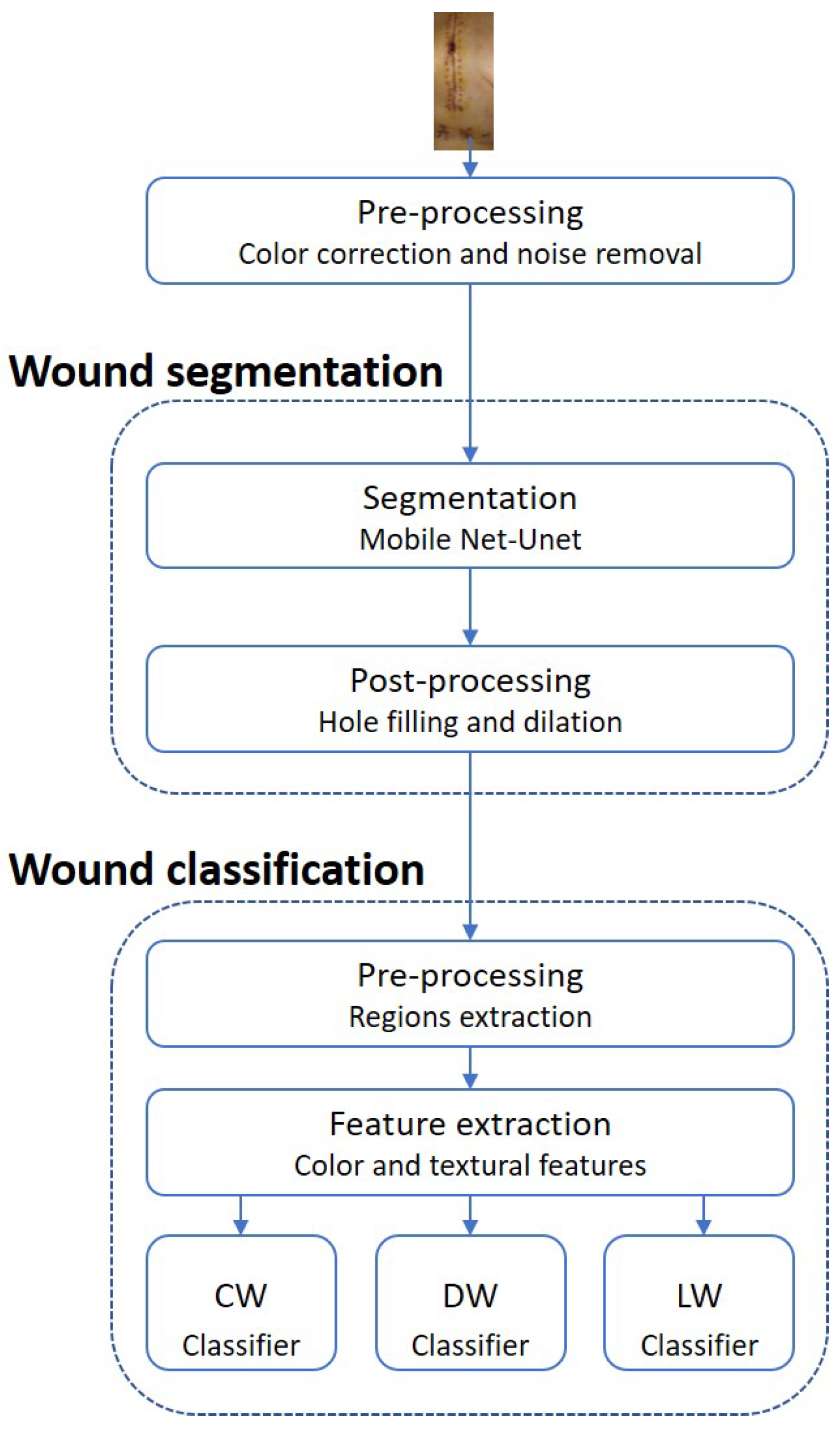
5.1. Wound Segmentation

MobileNet-Unet was the selected architecture for the wound segmentation model due to its good performance and advantageous characteristics. It achieved 82.06% ± 0.55% mean IoU when tested on the five test folds. MobileNet is a widely used structure with low memory requirements, high processing speed, and fewer parameters than other networks, which can be highly beneficial for this specific type of problem and for the future applications of this work. In terms of the decoder’s frameworks, there is no way to distinguish the best network because SegNet had a significantly better score than Unet for ResNet50 but worse for MobileNet, in which there is only a slight variance between both.

The reported results demonstrate that the Adam optimizer’s best batch size is 32, which is corroborated by [38], who suggested a 32 batch size was a reasonable default value. Commonly, larger batch sizes lead to poor generalization and can take a long to reach the optimal minimum. On the other hand, smaller batch sizes have shown faster convergence because they allow the model to start learning before seeing all data. Nevertheless, the model may never reach the optimal minimum. The presented outcomes on smaller batch sizes agree with several authors [39,40], which stated that a smaller batch size should be used. In addition, there is a high correlation between the learning rate and the batch size, where larger batch sizes perform better with high learning rates. In the present segmentation model, there was no optimization regarding the learning rate; the default values were 0.001 and 0.01 for Adam and SGD, respectively. Hence, these low learning rates demonstrated their better performance with the experimented small batch sizes. Regarding the optimizer’s choice, Adam is already an upgrade of SGD, which was proven for this dataset with the exhibited mean IoU. Regarding the reported results, the MobileNet-Unet architecture achieved its best performance with the Adam optimizer, a 32 batch size, and 50 epochs.

Data augmentation aims to improve the generalization of a model by artificially inflating the training dataset size with transformed data, introducing more information for the model to learn. However, the results remained the same with and without augmentation, concluding that the augmentation had no significant effect on the dataset. There are two possible explanations for this occurrence: a large number of data samples and the misrepresenting image transformations. Other combinations of geometrical and color modifications can be tried in the future to see if the model improves beyond its achieved performance.

Regarding the wound segmentation model, since the IoU metric penalizes the badly classified instances harder, it is the best metric to evaluate the proposed system along with the final mean average precision. It is vital not to have bad segmentation results since these can penalize and lead to wrong final classifications, such as FN, which can cause a wound with actual alterations to be overlooked by clinicians. Hence, it can be concluded that the segmentation system achieved a good score and performed well on the proposed task. The final average precision of the segmentation, 90.1%, shows promising results in the pixel-wise classification made by the segmentation model, which is extremely important for dividing the several wounds along the three classifiers. In addition, it indicates that the system seems suitable for our purpose.

5.2. Wound Classification

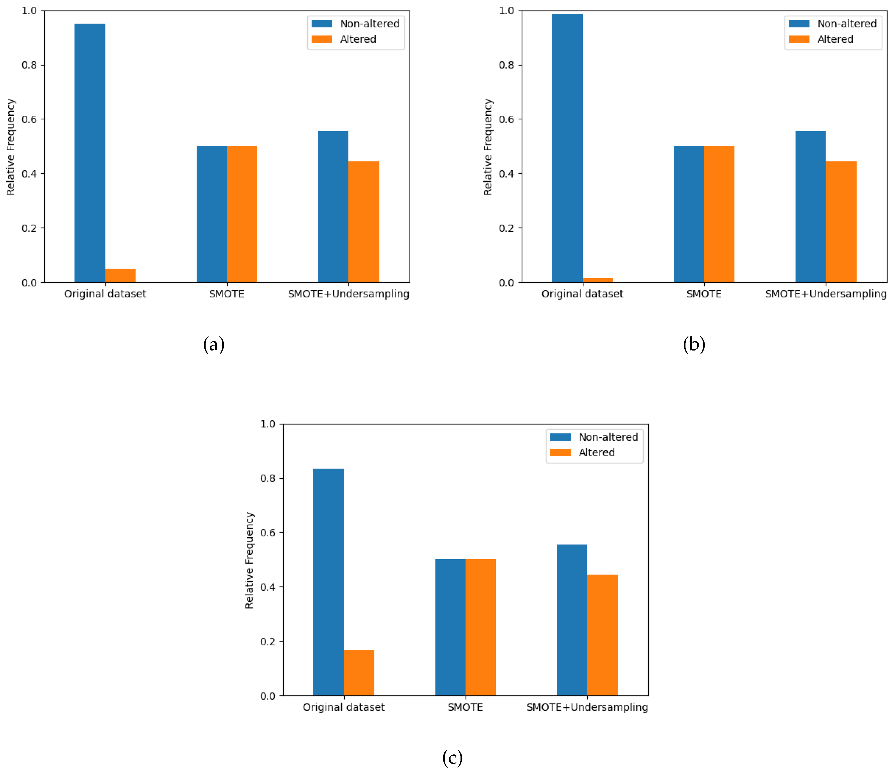
Applying methods that address class imbalance improves the performance of the models. In terms of the two trials conducted to balance the class distribution, the SMOTE technique combined with undersampling achieved better overall results than the single SMOTE method. However, the best type of technique to balance data is not equal for every classifier. The SMOTE technique had better scores for the LW classifier, while for CW and DW, the SMOTE + Undersampling was better. As the number of LW samples and the ratio between classes are smaller than in other wound types, the undersampling may eliminate important information regarding the negative class. Thus, the performance is slightly lower when compared to the use of SMOTE alone.

On the other hand, the CW and DW datasets are more extensive, so removing data points is less critical because there is more information regarding the majority class. Even though the oversampling techniques improved the model’s performance, some flaws must be considered. SMOTE generates a lot of noisy artificial samples in the feature space, which can increase the number of data points in the boundaries between the two classes, confusing the classification algorithm. In addition, the increase in samples may result in overfitting the model.

The number of features varies within each wound type classifier, suggesting that every wound type could have different representative features. Certain features may be more appropriate to characterize a specific wound type than another. However, the variance in the feature number is visible within the same type of classifier. Table 6, shows that the CW algorithm needs less number of components, 20 and 30, compared with the other types, indicating that the boundaries between the two classes are well-defined and that the alterations in the wounds are visually notorious.In contrast, DW needs more features to predict changes in the wound correctly and reports a lower performance when compared with the other classifiers. This can be interpreted as the substantial portion of the features extracted sharing similar values between the positive and negative classes, which can be explained by the few DW alterations being very hard to differentiate. Lastly, the LW algorithm varies the number of needed components from 50 to 60. It shows the best performance among the three classifiers, suggesting that the variations in the images between both classes are considerable and well-categorized.

The reported metrics of the wound alteration classifier show a high standard deviation, except for accuracy, due to the high number of obtained folds for validation and testing. Hence, the selection bias is minimal, but the evaluation performance variance is considerable. As expected, the models optimized with the F1 score have more balance between precision and recall, while the optimization with the F2 score compromises the precision to obtain a higher recall. All models achieved a good accuracy, but as mentioned, it is a biased metric even after the application of oversampling because the test data is unaltered; so, there is still a superior number of samples for the negative class.

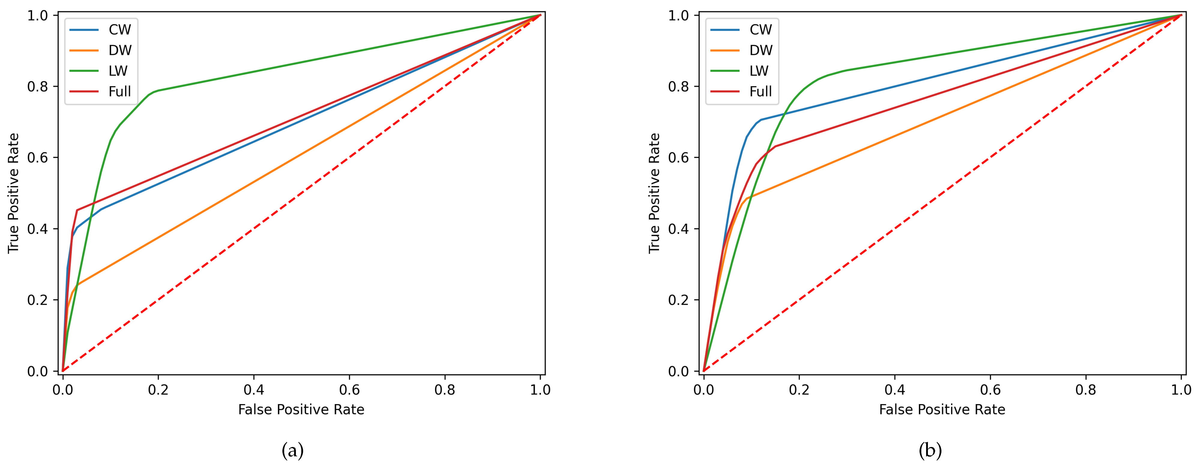
From all model types, the DW classifiers had the worst performance for both metrics, while LW achieved the best scores. Regarding the F1-optimization, DW obtained poor results, below 50%, for precision, recall, F1, and F2. The performance slightly improved for the F2-score, reaching a recall of 68.4%; however, the remaining metrics, except accuracy, still showed bad results. The poor results for the DW classifier can have two possible explanations: the significant discrepancy in the number of data samples between classes in the test set and the few differences presented between characteristics of positive and negative classes. The quantity of DW that has an alteration is low, meaning there are few examples of DW alterations. In CW, the scores already surpass the 50% barrier, except for the precision for the F2-optimization. The differences between F1 and F2 scores for both optimizers are low, while precision and recall are higher. Ultimately, the LW showed a higher overall score for all metrics and a recall of 87.6% for the F2-optimizer. However, it has the worst accuracy, which may be because LW has the lowest ratio between positive and negative classes; as such, the accuracy metric is less biased and corresponds more to reality.

The better performances by the LW and CW can be interpreted by the more considerable visual variances between the positive and negative classes, where the alterations of the wounds are more visible than in DW. It also corroborates that characteristics that indicate wound alterations can differ for each wound type, confirming the need to separate the wound classification problem into three classifiers.

Lastly, by comparing the performance between a single classifier and the three proposed, it can be concluded that the single classifier achieves a worse performance. Thus, it cannot be considered the final classification model.

The reported results and the discussion have some essential points of information that need to be addressed. As previously mentioned, a high number of FNs can be highly prejudicial to the proposed system, causing worrying alterations to be overlooked by the clinicians. For this reason, the best ML algorithms were selected based on the F2 optimization since it gives a higher weight to the recall metric. Hence, for the CW classifier, the RF algorithm with 50 feature components had the best performance with the following hyperparameters, entropy criterion, 1000 number of estimators, and with auto maximization of features. The SVM algorithm with regularization parameter (C) of 1, with rbf kernel type and an auto kernel coefficient (gamma), gave the best scores for the DW classifier with a total of 70 features. Lastly, the LW classifier utilized 60 features and elected the KNN algorithm with 5 nearest neighbors. The distance between them was measured by the minkowski metric, and the uniform weight function was used to make the predictions.

In summary, the LW clearly had the best performance, while the CW and DW need some improvements to obtain good predictions. As such, the LW classifier is acceptable for being implemented in the system, but overall, the classification needs improvement to be integrated into a real context. The use of oversampling techniques addresses the class imbalance problem by creating synthetic samples. However, the application of the SMOTE algorithm has to be cautious because artificially synthesized data may create unrealistic data samples that diverge from the actual dataset. Another essential consideration to consider is the lack of generalization present in the classification dataset. Besides the low amount of wounds belonging to the positive class, this reduced number is very biased because the same wound alteration is repeated for the same individual in the following images until a proposed treatment starts to have effects.

To the best of our knowledge, this is the first research work that applies artificial intelligent methods to assess surgical site infection in cardiac surgery based on images collected by patients themselves in a remote patient monitoring service. Related works were not trained with our type of wounds; most of them are related to burns or ulcers, which is the reason for not being able to present a fair comparison of our results with other related work.

5.3. Limitations

The size of the dataset may somewhat limit these findings. The dataset has a total of 1337 images. However, these belonged to a limited number of 34 patients, which may make the dataset redundant or ambiguous, showing slight variance among images. In addition, the number of images with alterations was significantly reduced, which constitutes a problem for ML algorithms because they have few examples to learn. Another limitation regarding the images was the uncontrolled illumination conditions when the images were taken, which could distort the results since one of the main characteristics of wound alterations is color. Even with these variances in illumination bringing robustness to the system, photographs with awful lighting conditions are detrimental to the system.

5.4. Future Work

Further research should be undertaken to investigate the use of other features for the wound alteration classification model, such as scale-invariant feature transform and histogram of oriented gradients, to verify their variance between the two classes and increase the performance of the classification model. Moreover, other undersampling techniques could be explored with the combination of SMOTE, such as Tomek links and edited nearest neighbour. Another possible solution would be a hybrid approach that extracts the features from the CNN layers and later feeds them into an ML algorithm.

In future investigations, it might be possible to assess a temporal evolution-based system that for each patient compares the daily image with the previous ones to assess the healing process regressed by analyzing if the wound shows more redness or abnormal coloration.

6. Conclusions

A system based on deep learning and machine learning methods for segmenting the wounds from daily patient photographs and classifying each post-surgical site as altered or not altered to prevent the risk of infection was designed and developed. The proposed system consists of two separate models, wound segmentation and wound classification, combining DL and traditional ML techniques. The segmentation model extracts the wound’s region areas and categorizes each of those regions with the corresponding wound type. This segmentation architecture showed promising results, with 89.9% of mean IoU after post-processing and a 90.1% mean average precision. A group of color and textural features was extracted from the output region of interest to feed one of the three wound-type classifiers that reached the final binary decision. Separating the final classification into separate classifiers was more effective than a single classifier for all the wound types. After hyperparameter search and model selection, the selected ML algorithms were RF, SVM, and KNN for CW, DW, and LW classifiers, respectively. The models were optimized in function of the F2 in order to favor the recall metric and of the F1 to find a balance solution with precision and recall. The best classifier (LW) obtained an 87.6% recall, 52.6% precision, 65.7% F1, and 77.3% F2. The appearance of FN could be a big issue for the system since it could overlook wound alterations and detect them negatively, preventing the intervention of the clinicians and increasing the risk of developing an infection. As such, the optimization with F2 was favored instead of F1.

References

1. Pezzella, A.T. Global Aspects of Cardiothoracic Surgery with Focus on Developing Countries. Asian Cardiovasc. Thorac. Ann. 2010, 18, 299–310. [Google Scholar] [CrossRef]
2. Segers, P.; de Jong, A.; Kloek, J.; Spanjaard, L.; de Mol, B. Risk control of surgical site infection after cardiothoracic surgery. J. Hosp. Infect. 2006, 62, 437–445. [Google Scholar] [CrossRef]
3. Jonkers, D. Prevalence of 90-days postoperative wound infections after cardiac surgery. Eur. J. Cardio-Thorac. Surg. 2003, 23, 97–102. [Google Scholar] [CrossRef] [PubMed]
4. L’Ecuyer, P.B.; Murphy, D.; Little, J.R.; Fraser, V.J. The Epidemiology of Chest and Leg Wound Infections Following Cardiothoracic Surgery. Clin. Infect. Dis. 1996, 22, 424–429. [Google Scholar] [CrossRef]
5. Ridderstolpe, L.; Gill, H.; Granfeldt, H.; Åhlfeldt, H.; Rutberg, H. Superficial and deep sternal wound complications: Incidence, risk factors and mortality. Eur. J. Cardio-Thorac. Surg. 2001, 20, 1168–1175. [Google Scholar] [CrossRef]
6. Zukowska, A.; Zukowski, M. Surgical Site Infection in Cardiac Surgery. J. Clin. Med. 2022, 11, 6991. [Google Scholar] [CrossRef] [PubMed]
7. Wang, C.; Yan, X.; Smith, M.; Kochhar, K.; Rubin, M.; Warren, S.M.; Wrobel, J.; Lee, H. A unified framework for automatic wound segmentation and analysis with deep convolutional neural networks. In Proceedings of the 2015 37th Annual International Conference of the IEEE Engineering in Medicine and Biology Society (EMBC), Milan, Italy, 25–29 August 2015. [Google Scholar] [CrossRef]
8. Goyal, M.; Yap, M.H.; Reeves, N.D.; Rajbhandari, S.; Spragg, J. Fully convolutional networks for diabetic foot ulcer segmentation. In Proceedings of the 2017 IEEE International Conference on Systems, Man, and Cybernetics (SMC), Banff, AB, Canada, 5–8 October 2017. [Google Scholar] [CrossRef]
9. Russakovsky, O.; Deng, J.; Su, H.; Krause, J.; Satheesh, S.; Ma, S.; Huang, Z.; Karpathy, A.; Khosla, A.; Bernstein, M.; et al. ImageNet Large Scale Visual Recognition Challenge. Int. J. Comput. Vis. 2015, 115, 211–252. [Google Scholar] [CrossRef]
10. Li, F.; Wang, C.; Liu, X.; Peng, Y.; Jin, S. A Composite Model of Wound Segmentation Based on Traditional Methods and Deep Neural Networks. Comput. Intell. Neurosci. 2018, 2018, 1–12. [Google Scholar] [CrossRef] [PubMed] [Green Version]
11. Liu, X.; Wang, C.; Li, F.; Zhao, X.; Zhu, E.; Peng, Y. A framework of wound segmentation based on deep convolutional networks. In Proceedings of the 2017 10th International Congress on Image and Signal Processing, BioMedical Engineering and Informatics (CISP-BMEI), Shanghai, China, 14–16 October 2017. [Google Scholar] [CrossRef]
12. Wang, C.; Anisuzzaman, D.M.; Williamson, V.; Dhar, M.K.; Rostami, B.; Niezgoda, J.; Gopalakrishnan, S.; Yu, Z. Fully automatic wound segmentation with deep convolutional neural networks. Sci. Rep. 2020, 10, 1–9. [Google Scholar] [CrossRef]
13. Cui, C.; Thurnhofer-Hemsi, K.; Soroushmehr, R.; Mishra, A.; Gryak, J.; Dominguez, E.; Najarian, K.; Lopez-Rubio, E. Diabetic Wound Segmentation using Convolutional Neural Networks. In Proceedings of the 2019 41st Annual International Conference of the IEEE Engineering in Medicine and Biology Society (EMBC), Berlin, Germany, 23–27 July 2019. [Google Scholar] [CrossRef]
14. Ohura, N.; Mitsuno, R.; Sakisaka, M.; Terabe, Y.; Morishige, Y.; Uchiyama, A.; Okoshi, T.; Shinji, I.; Takushima, A. Convolutional neural networks for wound detection: The role of artificial intelligence in wound care. J. Wound Care 2019, 28, S13–S24. [Google Scholar] [CrossRef]
15. Yadav, D.P.; Sharma, A.; Singh, M.; Goyal, A. Feature Extraction Based Machine Learning for Human Burn Diagnosis From Burn Images. IEEE J. Transl. Eng. Health Med. 2019, 7, 1–7. [Google Scholar] [CrossRef] [PubMed]
16. Suvarna, M.; Toney, G.; Swastik, G.B. Classification of scalding burn using image processing methods. In Proceedings of the 2017 International Conference on Intelligent Computing, Instrumentation and Control Technologies (ICICICT), Kerala, India, 6–7 July 2017. [Google Scholar] [CrossRef]
17. Beena, B.; Kumar, P. Diagnosis and Detection of Automatic Skin Burn Area Color Images Identification of Burn Area Depth in Color Images. Int. J. Eng. Trends Technol. 2017, 48, 48–54. [Google Scholar] [CrossRef]
18. Veredas, F.J.; Luque-Baena, R.M.; Martín-Santos, F.J.; Morilla-Herrera, J.C.; Morente, L. Wound image evaluation with machine learning. Neurocomputing 2015, 164, 112–122. [Google Scholar] [CrossRef]
19. Chakraborty, C. Computational approach for chronic wound tissue characterization. Informatics Med. Unlocked 2019, 17, 100162. [Google Scholar] [CrossRef]
20. Mukherjee, R.; Manohar, D.D.; Das, D.K.; Achar, A.; Mitra, A.; Chakraborty, C. Automated Tissue Classification Framework for Reproducible Chronic Wound Assessment. BioMed Res. Int. 2014, 2014, 1–9. [Google Scholar] [CrossRef] [Green Version]
21. Wada, K. labelme: Image Polygonal Annotation with Python. 2018. Available online: https://github.com/wkentaro/labelme (accessed on 27 November 2022).
22. Marijanović, D.; Filko, D. A systematic overview of recent methods for non-contact chronic wound analysis. Appl. Sci. 2020, 10, 7613. [Google Scholar] [CrossRef]
23. Land, E.H. The Retinex Theory of Color Vision The Retinex Theory of Color Vision of radiant energy but correlated with. Sci. Am. 1977, 237, 108–128. [Google Scholar] [CrossRef]
24. Kavitha, I.; Suganthi, S.S.; Ramakrishnan, S. Analysis of Chronic Wound Images Using Factorization Based Segmentation and Machine Learning Methods. In Proceedings of the 2017 International Conference on Computational Biology and Bioinformatics—ICCBB; ACM Press: New York, NY, USA, 2017. [Google Scholar] [CrossRef]
25. Gupta, D. Image Segmentation Keras: Implementation of Segnet, FCN, UNet, PSPNet and Other Models in Keras. 2019. Available online: https://github.com/divamgupta/image-segmentation-keras (accessed on 27 November 2022).
26. Howard, A.G.; Zhu, M.; Chen, B.; Kalenichenko, D.; Wang, W.; Weyand, T.; Andreetto, M.; Adam, H. MobileNets: Efficient Convolutional Neural Networks for Mobile Vision Applications. arXiv 2017, arXiv:1704.04861. [Google Scholar] [CrossRef]
27. He, K.; Zhang, X.; Ren, S.; Sun, J. Deep Residual Learning for Image Recognition. In Proceedings of the 2016 IEEE Conference on Computer Vision and Pattern Recognition (CVPR), Las Vegas, NV, USA, 27–30 June 2016. [Google Scholar] [CrossRef]
28. Ronneberger, O.; Fischer, P.; Brox, T. U-Net: Convolutional Networks for Biomedical Image Segmentation. IEEE Access 2015, 9, 16591–16603. [Google Scholar] [CrossRef]
29. Badrinarayanan, V.; Kendall, A.; Cipolla, R. Segnet: A deep convolutional encoder-decoder architecture for image segmentation. IEEE Trans. Pattern Anal. Mach. Intell. 2017, 39, 2481–2495. [Google Scholar] [CrossRef]
30. Jung, A.B.; Wada, K.; Crall, J.; Tanaka, S.; Graving, J.; Reinders, C.; Yadav, S.; Banerjee, J.; Vecsei, G.; Kraft, A.; et al. Imgaug. 2020. Available online: https://github.com/aleju/imgaug (accessed on 1 February 2020).
31. Lin, T.Y.; Maire, M.; Belongie, S.; Hays, J.; Perona, P.; Ramanan, D.; Dollár, P.; Zitnick, C.L. Microsoft COCO: Common Objects in Context. In Proceedings of the Computer Vision—ECCV 2014; Fleet, D., Pajdla, T., Schiele, B., Tuytelaars, T., Eds.; Springer International Publishing: Cham, Switzerland, 2014; pp. 740–755. [Google Scholar]
32. Giakoumoglou, N. PyFeats: Open Source Software for Image Feature Extraction. 2021. Available online: https://github.com/giakou4/pyfeats (accessed on 27 November 2022).
33. Stoecker, W.V.; Wronkiewiecz, M.; Chowdhury, R.; Stanley, R.J.; Xu, J.; Bangert, A.; Shrestha, B.; Calcara, D.A.; Rabinovitz, H.S.; Oliviero, M.; et al. Detection of granularity in dermoscopy images of malignant melanoma using color and texture features. Comput. Med. Imaging Graph. 2011, 35, 144–147. [Google Scholar] [CrossRef]
34. Haralick, R.M.; Shanmugam, K.; Dinstein, I. Textural Features for Image Classification. IEEE Trans. Syst. Man Cybern. 1973, SMC-3, 610–621. [Google Scholar] [CrossRef]
35. Liu, L.; Fieguth, P.; Guo, Y.; Wang, X.; Pietikäinen, M. Local binary features for texture classification: Taxonomy and experimental study. Pattern Recognit. 2017, 62, 135–160. [Google Scholar] [CrossRef] [Green Version]
36. Chawla, N.; Bowyer, K.; Hall, L.O.; Kegelmeyer, W.P. SMOTE: Synthetic Minority Over-sampling Technique. J. Artif. Intell. Res. 2002, 16, 321–357. [Google Scholar] [CrossRef]
37. Fawcett, T. An introduction to ROC analysis. Pattern Recognit. Lett. 2006, 27, 861–874. [Google Scholar] [CrossRef]
38. Bengio, Y. Practical Recommendations for Gradient-Based Training of Deep Architectures. In Lecture Notes in Computer Science; Springer: Berlin/Heidelberg, Germany, 2012; pp. 437–478. [Google Scholar] [CrossRef]
39. Kandel, I.; Castelli, M. The effect of batch size on the generalizability of the convolutional neural networks on a histopathology dataset. ICT Express 2020, 6, 312–315. [Google Scholar] [CrossRef]
40. Masters, D.; Luschi, C. Revisiting Small Batch Training for Deep Neural Networks. arXiv 2018, arXiv:1804.07612. [Google Scholar] [CrossRef]
Figure 1. Different types of wounds: (a) example of chest wound labelled as CW; (b) example of drainage wound labelled as DW; (c) example of leg wound labelled as LW.
Applsci 13 02120 g001
Figure 2. Example of wound categories: (a) example of chest wound without alarmist alteration labelled as NO; (b) example of chest wound with alarmist alteration, labelled as YES.
Applsci 13 02120 g002
Figure 3. Process of the flowchart of the proposed system. CW is chest wound, DW drainage wound, and LW leg wound.
Applsci 13 02120 g003
Figure 4. Example of image result from the pre-processing step: (a) original image before pre-processing; (b) image after pre-processing.
Applsci 13 02120 g004
Figure 5. Representation of the nested cross-validation procedure.
Applsci 13 02120 g005
Figure 6. Example of a final output image from the segmentation model.
Applsci 13 02120 g006
Figure 7. Class distribution over the three wound types, before and after the approaches to address class imbalance: (a) CW type; (b) DW type; (c) LW type.
Applsci 13 02120 g007
Figure 8. Receiving operating characteristic (ROC) curves of each classifier model: CW is chest wound, DW drainage wound, LW leg wound, and full dataset: (a) ROC curves optimized regarding F1 score; (b) ROC curves optimized regarding F2 score.
Applsci 13 02120 g008