
Deep Cellular Automata-Based Feature Extraction for Classification of the Breast Cancer Image


Abstract
:1. Introduction
2. Background
2.1. Deep Feature Learning in Images
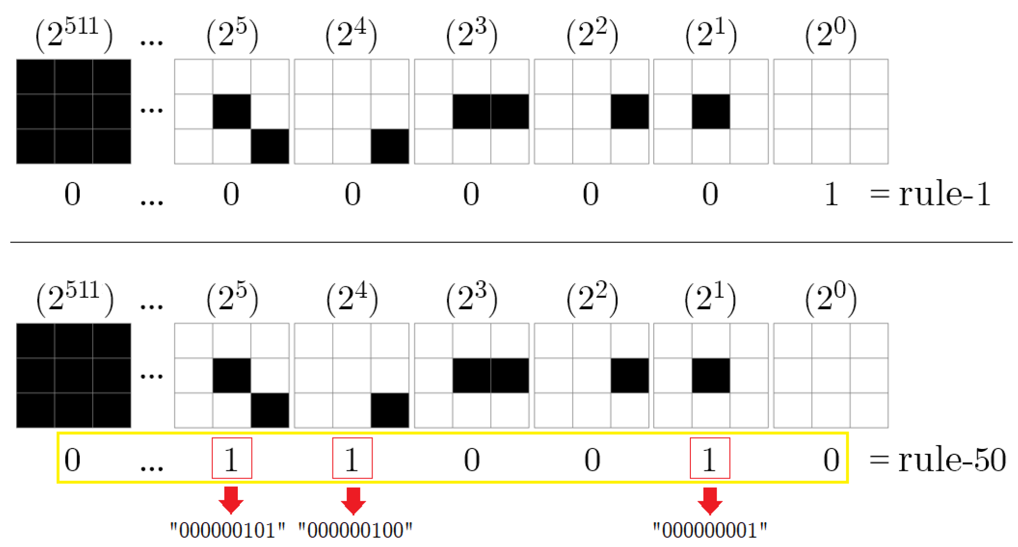
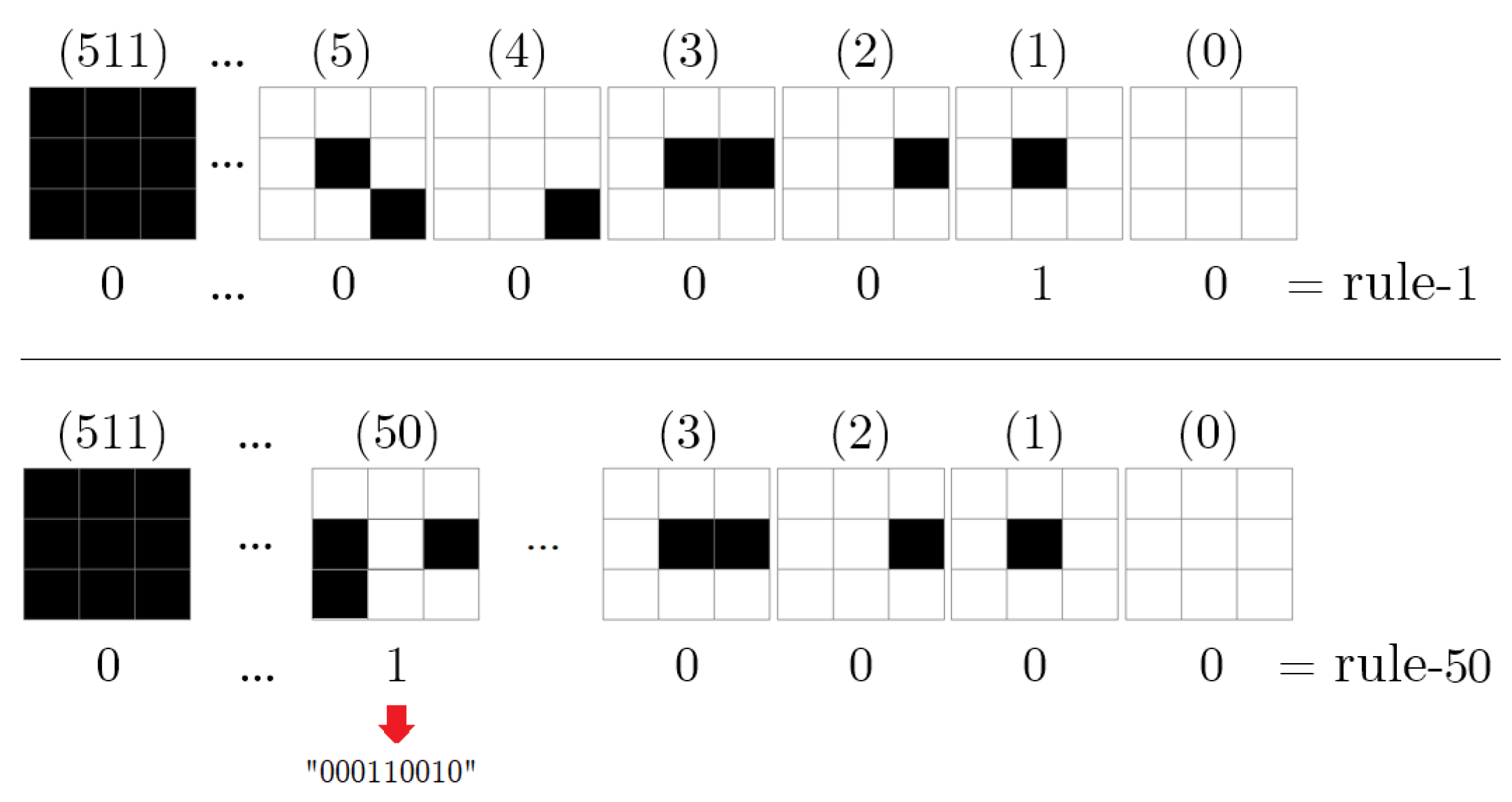
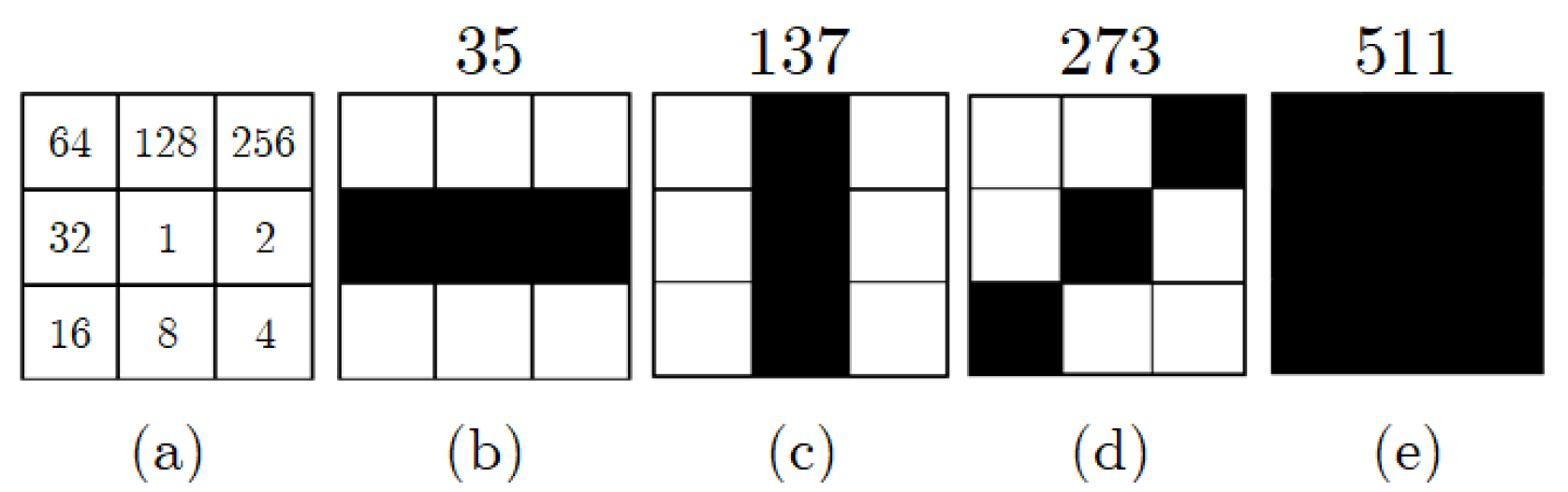
2.2. Cellular Automata (CA)
3. Proposed Method
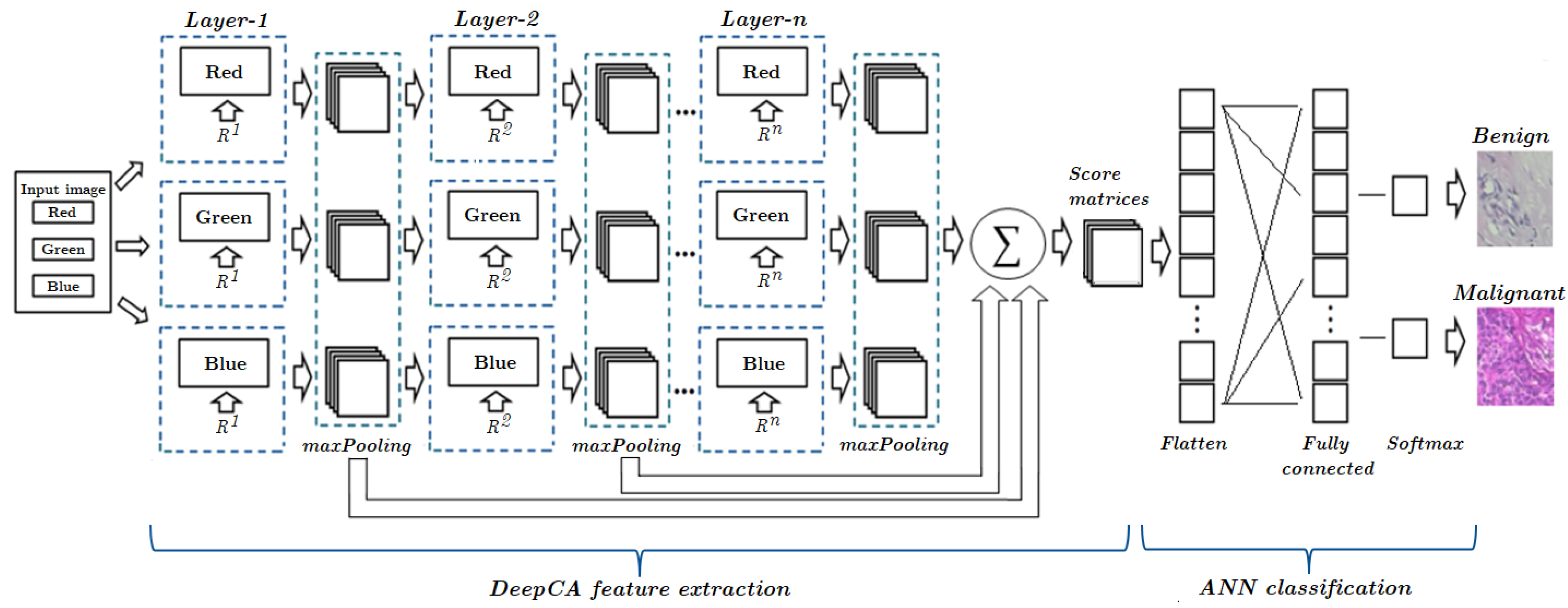
3.1. Basics of DeepCA Feature Extraction
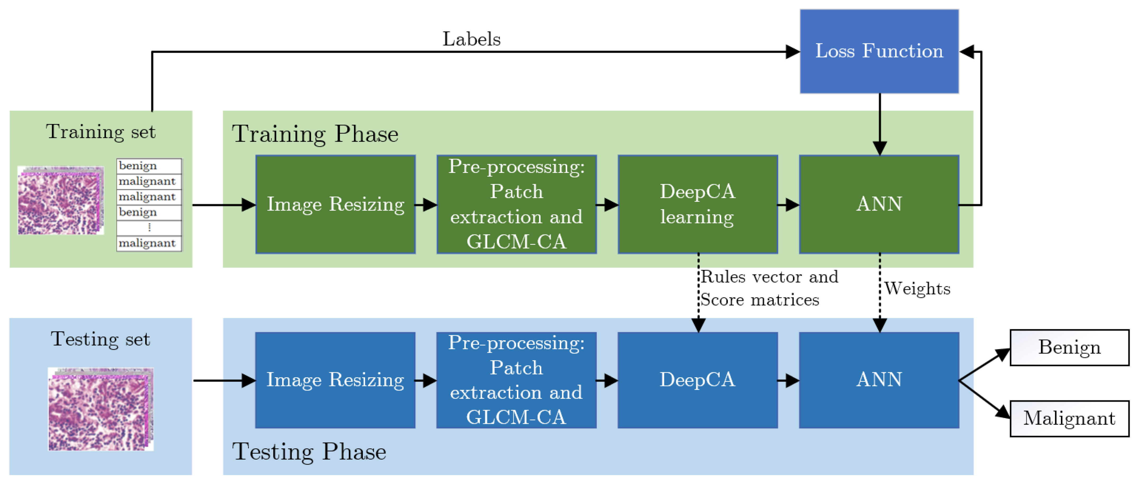
3.2. Proposed Framework
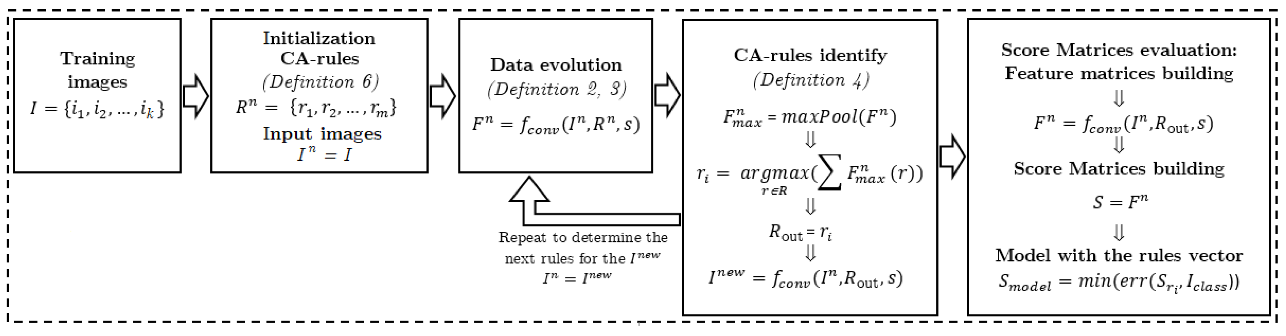
| Algorithm 1: Training algorithm for DeepCA. |
 |
3.3. DeepCA Training
4. Experiments and Results
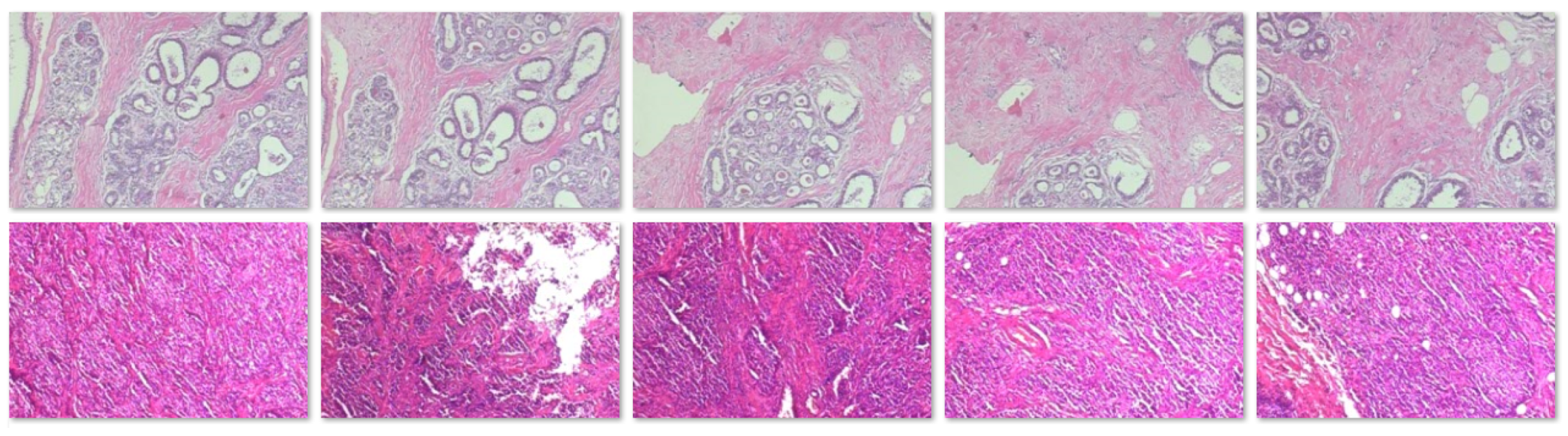
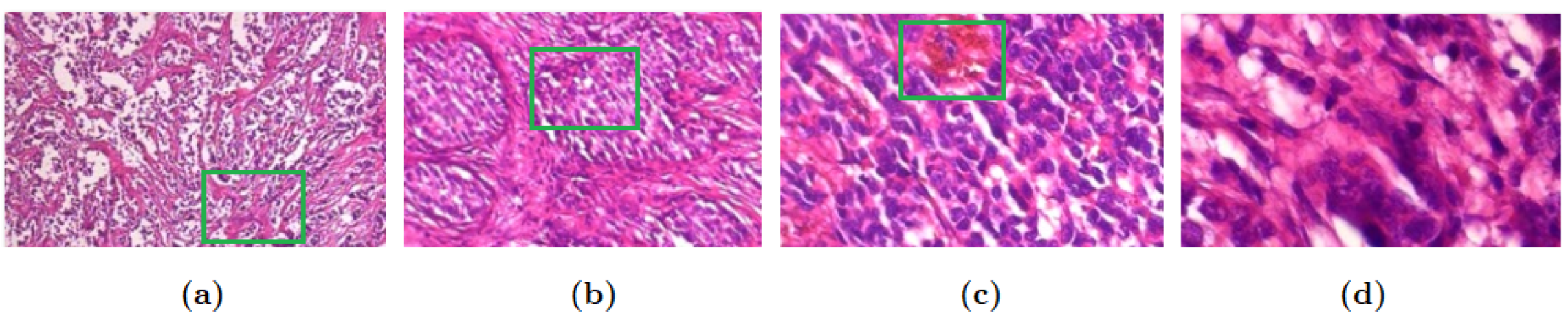
4.1. Dataset
4.2. Training Parameters of the Classifier
4.3. Performance Evaluation
4.4. Results
4.5. Discussions
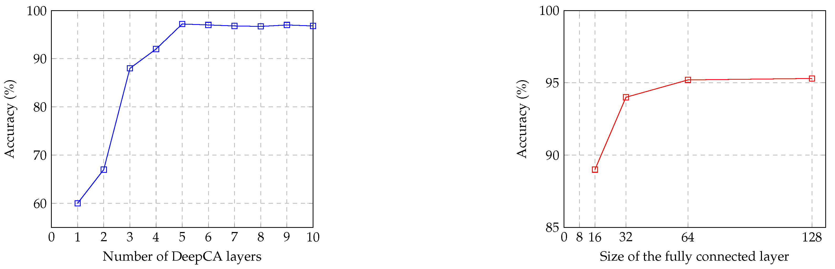
4.6. Parameter Sensitivity
5. Conclusions
Author Contributions
Funding
Institutional Review Board Statement
Informed Consent Statement
Data Availability Statement
Acknowledgments
Conflicts of Interest
Abbreviations
| 1-NN | 1-nearest neighbor |
| ANN | Artificial Neural Network |
| CA | Cellular Automata |
| CAT | Computer-Aided Tomography |
| CLBPs | Completed local binary patterns |
| CNN | Convolutional Neural Networks |
| CSAE | Convolutional sparse autoencoder |
| DBT | Digital breast tomosynthesis |
| DCNN | Deep convolutional neural networks |
| DeepCA | Deep cellular automata |
| ECA | Elementary cellular automaton |
| FCNNs | Fully connected neural networks |
| GLCMs | Grey-level co-occurrence matrices |
| LBPs | Local binary patterns |
| MIL | Multiple-instance learning |
| MLP | Multilayer perceptrons (MLP) |
| MRI | Magnetic Resonance Imaging |
| PFTASs | Threshold adjacency statistics |
| QDA | Quadratic linear analysis |
| RF | Random forest |
| SSAE | Stacked sparse autoencoder |
| SVMs | Support vector machines |
| VLAD | Vector of locally aggregated descriptors |
References
- Skandalakis, J.E. Embryology and anatomy of the breast. In Breast Augmentation; Springer: Berlin/Heidelberg, Germany, 2009; pp. 3–24. [Google Scholar] [CrossRef]
- Ellis, H.; Colborn, G.L.; Skandalakis, J.E. Surgical embryology and anatomy of the breast and its related anatomic structures. Surg. Clin. North Am. 1993, 73, 611. [Google Scholar] [CrossRef] [PubMed]
- Rubin, R.; Strayer, D.S.; Rubin, E. Rubin’s Pathology: Clinicopathologic Foundations of Medicine; Lippincott Williams & Wilkins: Philadelphia, PA, USA, 2008. [Google Scholar]
- Lakhani, S.R.; Ellis, I.O.; Schnitt, S.; Tan, P.H.; van de Vijver, M. WHO Classification of Tumours of the Breast; IARC: Lyon, France, 2012. [Google Scholar]
- Spanhol, F.A.; Oliveira, L.S.; Petitjean, C.; Heutte, L. A dataset for breast cancer histopathological image classification. IEEE Trans. Biomed. Eng. 2015, 63, 1455–1462. [Google Scholar] [CrossRef] [PubMed]
- Haralick, R.M.; Shanmugam, K.; Dinstein, I.H. Textural features for image classification. IEEE Trans. Syst. Man Cybern. 1973, 6, 610–621. [Google Scholar] [CrossRef]
- Ojala, T.; Pietikainen, M.; Maenpaa, T. Multiresolution gray-scale and rotation invariant texture classification with local binary patterns. IEEE Trans. Pattern Anal. Mach. Intell. 2002, 24, 971–987. [Google Scholar] [CrossRef]
- Hamilton, N.A.; Pantelic, R.S.; Hanson, K.; Teasdale, R.D. Fast automated cell phenotype image classification. BMC Bioinform. 2007, 8, 110. [Google Scholar] [CrossRef]
- Ojansivu, V.; Heikkilä, J. Blur insensitive texture classification using local phase quantization. In Proceedings of the International Conference on Image and Signal Processing, Cherbourg-Octeville, France, 1–3 July 2008; Springer: Berlin/Heidelberg, Germany, 2008; pp. 236–243. [Google Scholar] [CrossRef]
- Guo, Z.; Zhang, L.; Zhang, D. A completed modeling of local binary pattern operator for texture classification. IEEE Trans. Image Process. 2010, 19, 1657–1663. [Google Scholar] [CrossRef]
- Rublee, E.; Rabaud, V.; Konolige, K.; Bradski, G. ORB: An efficient alternative to SIFT or SURF. In Proceedings of the 2011 International Conference on Computer Vision, Barcelona, Spain, 6–13 November 2011; pp. 2564–2571. [Google Scholar] [CrossRef]
- Agarwal, N.; Ford, K.H.; Shneider, M. Sentence boundary detection using a maxEnt classifier. Proc. MISC 2005, 1–6. [Google Scholar]
- Mohammed, N.F.; Omar, N. Arabic named entity recognition using artificial neural network. J. Comput. Sci. 2012, 8, 1285. [Google Scholar]
- Perboli, G.; Gajetti, M.; Fedorov, S.; Giudice, S.L. Natural language processing for the identification of human factors in aviation accidents causes: An application to the SHEL methodology. Expert Syst. Appl. 2021, 186, 115694. [Google Scholar] [CrossRef]
- Sompong, C.; Wongthanavasu, S. An efficient brain tumor segmentation based on cellular automata and improved tumor-cut algorithm. Expert Syst. Appl. 2017, 72, 231–244. [Google Scholar] [CrossRef]
- Zhang, Z.; Wu, Z.; Jiang, Q.; Du, L.; Hu, L. Co-saliency Detection Based on Superpixel Matching and Cellular Automata. TIIS 2017, 11, 2576–2589. [Google Scholar] [CrossRef]
- Liu, Y.; Yuan, P. Saliency Detection Using Global and Local Information Under Multilayer Cellular Automata. IEEE Access 2019, 7, 72736–72748. [Google Scholar] [CrossRef]
- LeCun, Y.; Bottou, L.; Bengio, Y.; Haffner, P. Gradient-based learning applied to document recognition. Proc. IEEE 1998, 86, 2278–2324. [Google Scholar] [CrossRef]
- Krizhevsky, A.; Sutskever, I.; Hinton, G.E. Imagenet classification with deep convolutional neural networks. In Proceedings of the Advances in Neural Information Processing Systems, San Francisco, CA, USA, 30 November–3 December 1992; pp. 1097–1105. [Google Scholar]
- LeCun, Y.; Bengio, Y.; Hinton, G. Deep learning. Nature 2015, 521, 436–444. [Google Scholar] [CrossRef]
- Nichele, S.; Molund, A. Deep learning with cellular automaton-based reservoir computing. Complex Systems 2017, 26, 319–340. [Google Scholar] [CrossRef]
- Tangsakul, S.; Wongthanavasu, S. Single Image Haze Removal Using Deep Cellular Automata Learning. IEEE Access 2020, 8, 103181–103199. [Google Scholar] [CrossRef]
- Zhang, B. Breast cancer diagnosis from biopsy images by serial fusion of Random Subspace ensembles. In Proceedings of the 2011 4th International Conference on Biomedical Engineering and Informatics (BMEI), Shanghai, China, 15–17 October 2011; Volume 1, pp. 180–186. [Google Scholar] [CrossRef]
- Dimitropoulos, K.; Barmpoutis, P.; Zioga, C.; Kamas, A.; Patsiaoura, K.; Grammalidis, N. Grading of invasive breast carcinoma through Grassmannian VLAD encoding. PLoS ONE 2017, 12, e0185110. [Google Scholar] [CrossRef]
- Alirezazadeh, P.; Hejrati, B.; Monsef-Esfahani, A.; Fathi, A. Representation learning-based unsupervised domain adaptation for classification of breast cancer histopathology images. Biocybern. Biomed. Eng. 2018, 38, 671–683. [Google Scholar] [CrossRef]
- Albarqouni, S.; Baur, C.; Achilles, F.; Belagiannis, V.; Demirci, S.; Navab, N. Aggnet: Deep learning from crowds for mitosis detection in breast cancer histology images. IEEE Trans. Med. Imaging 2016, 35, 1313–1321. [Google Scholar] [CrossRef]
- Suzuki, S.; Zhang, X.; Homma, N.; Ichiji, K.; Sugita, N.; Kawasumi, Y.; Ishibashi, T.; Yoshizawa, M. Mass detection using deep convolutional neural network for mammographic computer-aided diagnosis. In Proceedings of the 2016 55th Annual Conference of the Society of Instrument and Control Engineers of Japan (SICE), Tsukuba, Japan, 20–23 September 2016; pp. 1382–1386. [Google Scholar]
- Ertosun, M.G.; Rubin, D.L. Probabilistic visual search for masses within mammography images using deep learning. In Proceedings of the 2015 IEEE International Conference on Bioinformatics and Biomedicine (BIBM), Washington, DC, USA, 9–12 November 2015; pp. 1310–1315. [Google Scholar] [CrossRef]
- Spanhol, F.A.; Oliveira, L.S.; Cavalin, P.R.; Petitjean, C.; Heutte, L. Deep features for breast cancer histopathological image classification. In Proceedings of the 2017 IEEE International Conference on Systems, Man, and Cybernetics (SMC), Banff, AB, Canada, 5–8 October 2017; pp. 1868–1873. [Google Scholar] [CrossRef]
- Xu, J.; Xiang, L.; Hang, R.; Wu, J. Stacked Sparse Autoencoder (SSAE) based framework for nuclei patch classification on breast cancer histopathology. In Proceedings of the 2014 IEEE 11th International Symposium on Biomedical Imaging (ISBI), Beijing, China, 29 Apri–2 May 2014; pp. 999–1002. [Google Scholar] [CrossRef]
- Jia, Y.; Shelhamer, E.; Donahue, J.; Karayev, S.; Long, J.; Girshick, R.; Guadarrama, S.; Darrell, T. Caffe: Convolutional architecture for fast feature embedding. In Proceedings of the 22nd ACM International Conference on Multimedia, Orlando, FL, USA, 3–7 November 2014; pp. 675–678. [Google Scholar] [CrossRef]
- Dhungel, N.; Carneiro, G.; Bradley, A.P. Deep structured learning for mass segmentation from mammograms. In Proceedings of the 2015 IEEE International Conference on Image Processing (ICIP), Quebec City, QC, Canada, 27–30 September 2015; pp. 2950–2954. [Google Scholar] [CrossRef]
- Deng, J.; Dong, W.; Socher, R.; Li, L.J.; Li, K.; Fei-Fei, L. Imagenet: A large-scale hierarchical image database. In Proceedings of the 2009 IEEE Conference on Computer Vision and Pattern Recognition, Miami, FL, USA, 20–25 June 2009; pp. 248–255. [Google Scholar] [CrossRef]
- Kallenberg, M.; Petersen, K.; Nielsen, M.; Ng, A.Y.; Diao, P.; Igel, C.; Vachon, C.M.; Holland, K.; Winkel, R.R.; Karssemeijer, N.; et al. Unsupervised deep learning applied to breast density segmentation and mammographic risk scoring. IEEE Trans. Med. Imaging 2016, 35, 1322–1331. [Google Scholar] [CrossRef]
- Kim, D.H.; Kim, S.T.; Ro, Y.M. Latent feature representation with 3-D multi-view deep convolutional neural network for bilateral analysis in digital breast tomosynthesis. In Proceedings of the 2016 IEEE International Conference on Acoustics, Speech and Signal Processing (ICASSP), Shanghai, China, 20–25 March 2016; pp. 927–931. [Google Scholar] [CrossRef]
- Swiderski, B.; Kurek, J.; Osowski, S.; Kruk, M.; Barhoumi, W. Deep learning and non-negative matrix factorization in recognition of mammograms. In Proceedings of the Eighth International Conference on Graphic and Image Processing (ICGIP 2016), Tokyo, Japan, 29–31 October 2016; International Society for Optics and Photonics: Bellingham, WA, USA, 2017; Volume 10225, p. 102250B. [Google Scholar] [CrossRef]
- Sudharshan, P.; Petitjean, C.; Spanhol, F.; Oliveira, L.E.; Heutte, L.; Honeine, P. Multiple instance learning for histopathological breast cancer image classification. Expert Syst. Appl. 2019, 117, 103–111. [Google Scholar] [CrossRef]
- Saini, M.; Susan, S. Deep transfer with minority data augmentation for imbalanced breast cancer dataset. Appl. Soft Comput. 2020, 97, 106759. [Google Scholar] [CrossRef]
- Saxena, S.; Shukla, S.; Gyanchandani, M. Breast cancer histopathology image classification using kernelized weighted extreme learning machine. Int. J. Imaging Syst. Technol. 2021, 31, 168–179. [Google Scholar] [CrossRef]
- Li, X.; Shen, X.; Zhou, Y.; Wang, X.; Li, T.Q. Classification of breast cancer histopathological images using interleaved DenseNet with SENet (IDSNet). PLoS ONE 2020, 15, e0232127. [Google Scholar] [CrossRef]
- Sharma, S.; Kumar, S. The Xception model: A potential feature extractor in breast cancer histology images classification. ICT Express 2022, 8, 101–108. [Google Scholar] [CrossRef]
- Hao, Y.; Zhang, L.; Qiao, S.; Bai, Y.; Cheng, R.; Xue, H.; Hou, Y.; Zhang, W.; Zhang, G. Breast cancer histopathological images classification based on deep semantic features and gray level co-occurrence matrix. PLoS ONE 2022, 17, e0267955. [Google Scholar] [CrossRef]
- Atban, F.; Ekinci, E.; Garip, Z. Traditional machine learning algorithms for breast cancer image classification with optimized deep features. Biomed. Signal Process. Control. 2023, 81, 104534. [Google Scholar] [CrossRef]
- Neumann, J.; Burks, A.W. Theory of self-reproducing automata; University of Illinois Press Urbana: Champaign, IL, USA, 1966; Volume 1102024. [Google Scholar]
- Ulam, S. Some ideas and prospects in biomathematics. Annu. Rev. Biophys. Bioeng. 1972, 1, 277–292. [Google Scholar] [CrossRef] [PubMed]
- Wolfram, S. Computation theory of cellular automata. Commun. Math. Phys. 1984, 96, 15–57. [Google Scholar] [CrossRef]
- Sahin, U.; Uguz, S.; Sahin, F. Salt and pepper noise filtering with fuzzy-cellular automata. Comput. Electr. Eng. 2014, 40, 59–69. [Google Scholar] [CrossRef]
- Wongthanavasu, S.; Sadananda, R. A CA-based edge operator and its performance evaluation. J. Vis. Commun. Image Represent. 2003, 14, 83–96. [Google Scholar] [CrossRef]
- Kumar, T.; Sahoo, G. A novel method of edge detection using cellular automata. Int. J. Comput. Appl. 2010, 9, 38–44. [Google Scholar] [CrossRef]
- Rosin, P.L.; Sun, X. Edge detection using cellular automata. In Cellular Automata in Image Processing and Geometry; Springer: Cham, Switzerland, 2014; pp. 85–103. [Google Scholar] [CrossRef]
- Diwakar, M.; Patel, P.K.; Gupta, K. Cellular automata based edge-detection for brain tumor. In Proceedings of the 2013 International Conference on Advances in Computing, Communications and Informatics (ICACCI), Mysore, India, 22–25 August 2013; pp. 53–59. [Google Scholar] [CrossRef]
- Tourtounis, D.; Mitianoudis, N.; Sirakoulis, G.C. Salt-n-pepper noise filtering using cellular automata. arXiv 2017, arXiv:1708.05019. [Google Scholar]
- Qadir, F.; Shoosha, I.Q. Cellular automata-based efficient method for the removal of high-density impulsive noise from digital images. Int. J. Inf. Technol. 2018, 10, 529–536. [Google Scholar] [CrossRef]
- Priego, B.; Prieto, A.; Duro, R.J.; Chanussot, J. A cellular automata-based filtering approach to multi-temporal image denoising. Expert Syst. 2018, 35, e12235. [Google Scholar] [CrossRef]
- Qin, Y.; Feng, M.; Lu, H.; Cottrell, G.W. Hierarchical cellular automata for visual saliency. Int. J. Comput. Vis. 2018, 126, 751–770. [Google Scholar] [CrossRef]
- Liu, Y.; Chen, Y.; Han, B.; Zhang, Y.; Zhang, X.; Su, Y. Fully automatic Breast ultrasound image segmentation based on fuzzy cellular automata framework. Biomed. Signal Process. Control. 2018, 40, 433–442. [Google Scholar] [CrossRef]
- Li, C.; Liu, L.; Sun, X.; Zhao, J.; Yin, J. Image segmentation based on fuzzy clustering with cellular automata and features weighting. EURASIP J. Image Video Process. 2019, 2019, 1–11. [Google Scholar] [CrossRef]
- Wali, A.; Saeed, M. Biologically inspired cellular automata learning and prediction model for handwritten pattern recognition. Biol. Inspired Cogn. Archit. 2018, 24, 77–86. [Google Scholar] [CrossRef]
- Packard, N.H.; Wolfram, S. Two-dimensional cellular automata. J. Stat. Phys. 1985, 38, 901–946. [Google Scholar] [CrossRef]
- Khan, A.R.; Choudhury, P.P.; Dihidar, K.; Mitra, S.; Sarkar, P. VLSI architecture of a cellular automata machine. Comput. Math. Appl. 1997, 33, 79–94. [Google Scholar] [CrossRef]
- Uguz, S.; Akin, H.; Siap, I.; Sahin, U. On the irreversibility of Moore cellular automata over the ternary field and image application. Appl. Math. Model. 2016, 40, 8017–8032. [Google Scholar] [CrossRef]
- Jana, B.; Pal, P.; Bhaumik, J. New image noise reduction schemes based on cellular automata. Int. J. Soft Comput. Eng. 2012, 2, 98–103. [Google Scholar]
- Murphy, K.P. Machine Learning: A Probabilistic Perspective; MIT Press: Cambridge, MA, USA, 2012. [Google Scholar]
- Spanhol, F.A.; Oliveira, L.S.; Petitjean, C.; Heutte, L. Breast cancer histopathological image classification using convolutional neural networks. In Proceedings of the 2016International Joint Conference on Neural Networks (IJCNN), Vancouver, BC, Canada, 24–29 July 2016; pp. 2560–2567. [Google Scholar] [CrossRef]
- Bayramoglu, N.; Kannala, J.; Heikkilä, J. Deep learning for magnification independent breast cancer histopathology image classification. In Proceedings of the 2016 23rd International Conference on Pattern Recognition (ICPR), Cancun, Mexico, 4–8 December 2016; pp. 2440–2445. [Google Scholar] [CrossRef]
- Mehra, R. Automatic magnification independent classification of breast cancer tissue in histological images using deep convolutional neural network. In Proceedings of the International Conference on Advanced Informatics for Computing Research, Shimla, India, 14–15 July 2018; Springer: Singapore, 2018; pp. 772–781. [Google Scholar] [CrossRef]
- Nahid, A.A.; Kong, Y. Histopathological breast-image classification using local and frequency domains by convolutional neural network. Information 2018, 9, 19. [Google Scholar] [CrossRef]


| Magnification | Benign | Malignant | Total |
|---|---|---|---|
| 40× | 625 | 1370 | 1995 |
| 100× | 644 | 1437 | 2081 |
| 200× | 623 | 1390 | 2013 |
| 400× | 588 | 1232 | 1820 |
| Total | 2480 | 5429 | 7909 |
| Patients | 24 | 58 | 82 |
| Methods | Size of the Input Layer | No. and Sizes of Fully Connected Layers | Size of the Ooutput Layer |
|---|---|---|---|
| Proposed method 1 | 12,288 | 1:64 | 2 |
| Proposed method 2 | 12,288 | 2:64, 64 | 2 |
| Proposed method 3 | 12,288 | 3:64, 64, 32 | 2 |
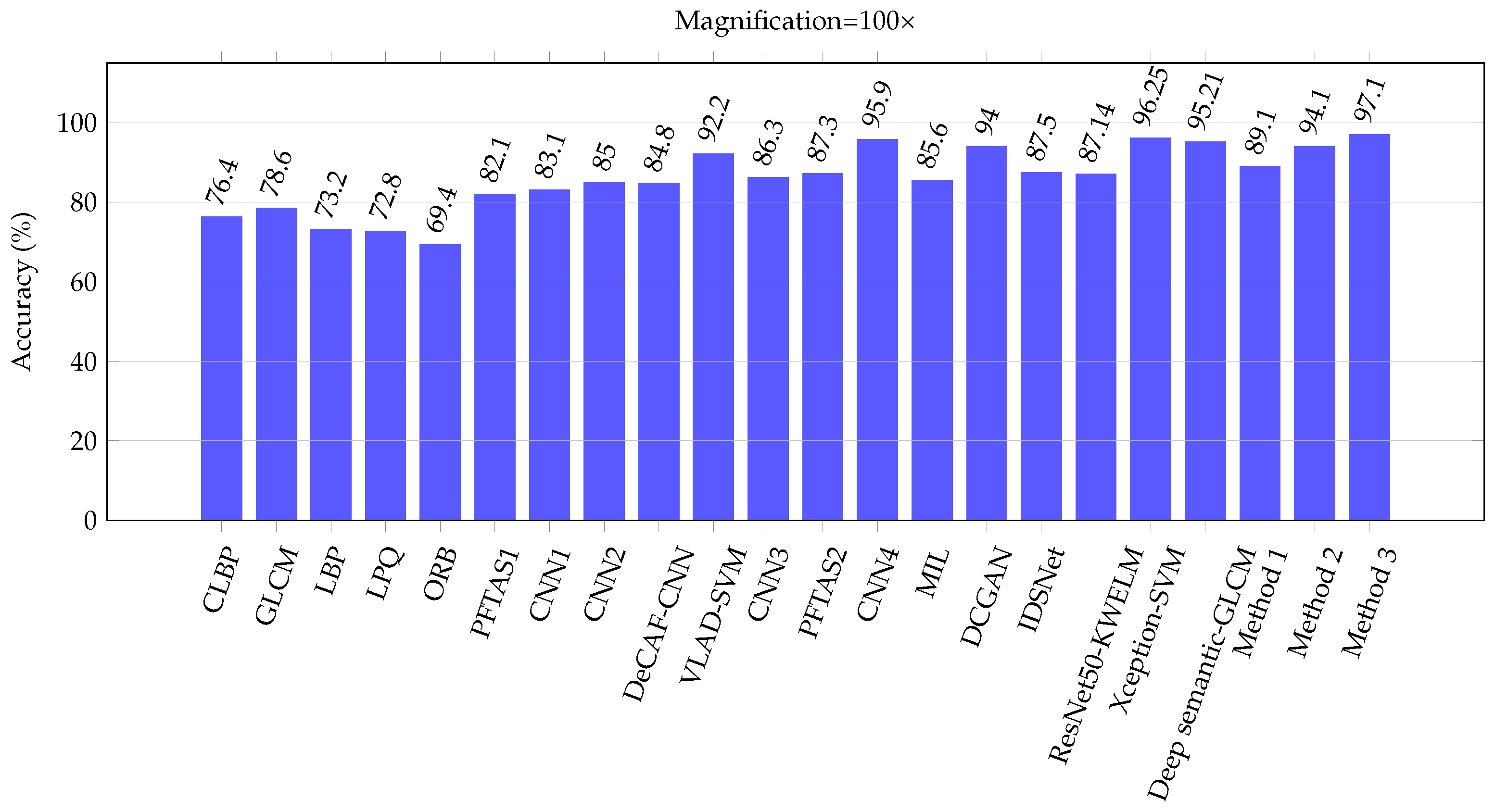
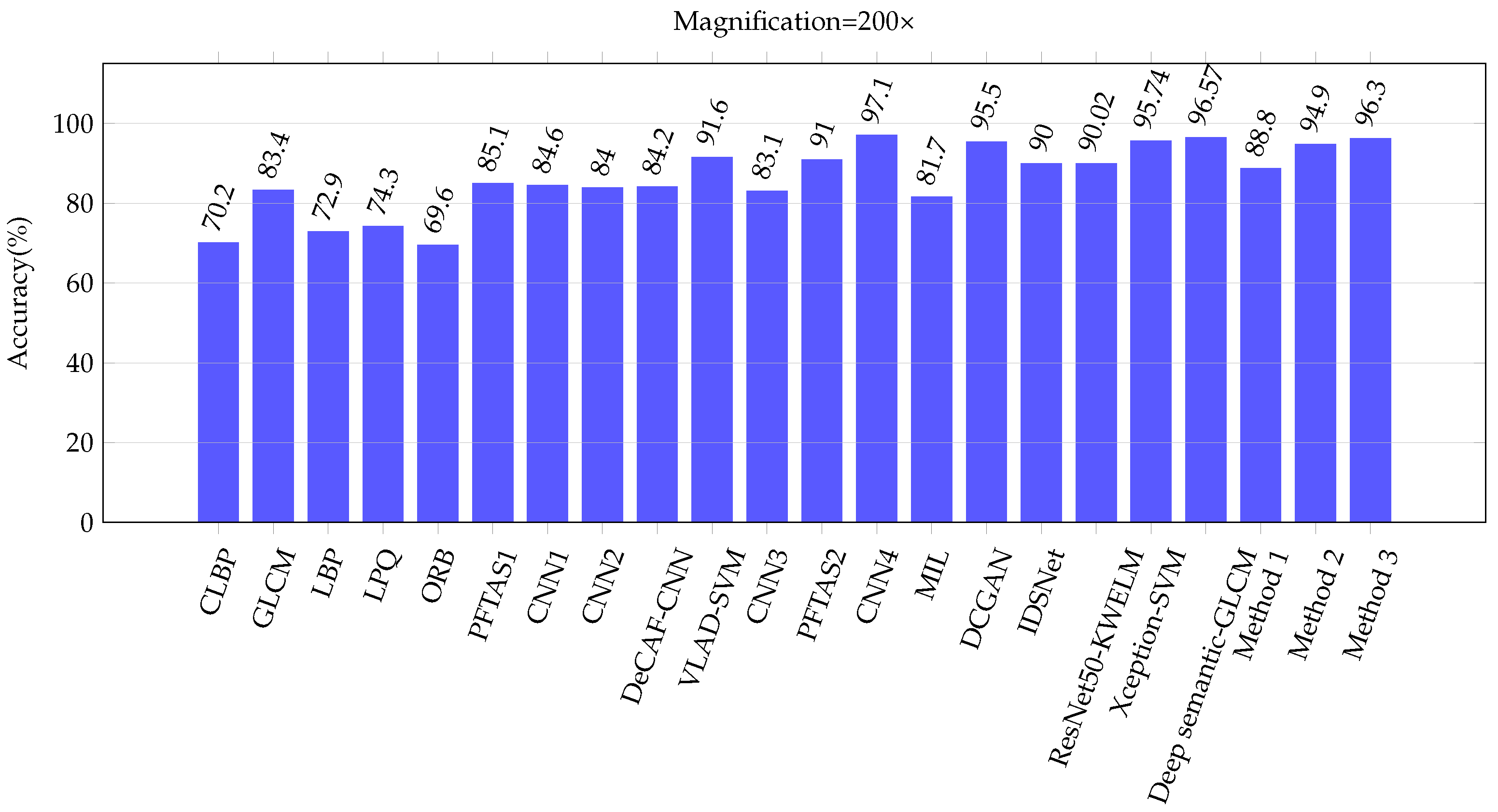
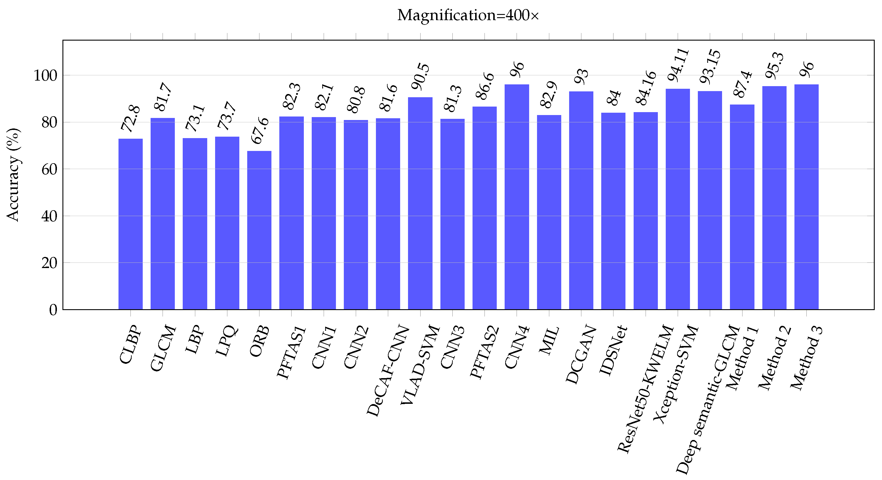
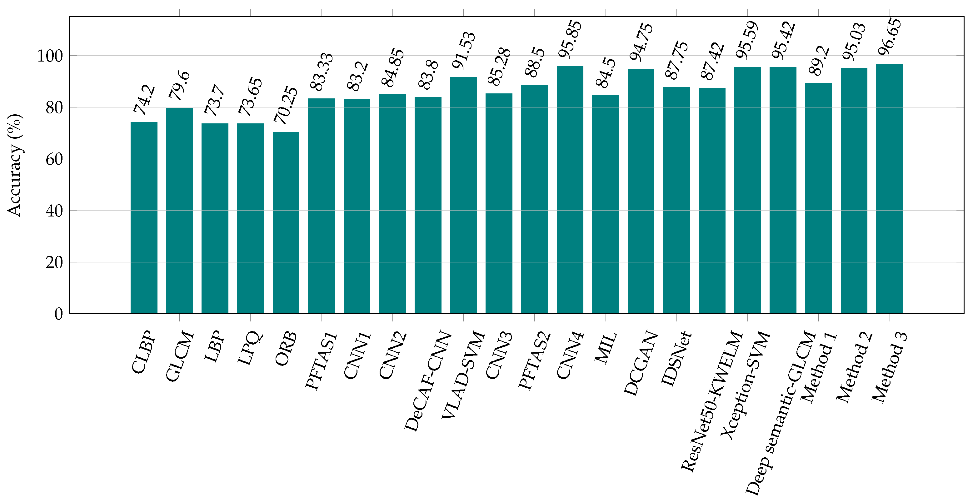
| Methods | Authors | Magnification Factors | Average | |||
|---|---|---|---|---|---|---|
| 40× | 100× | 200× | 400× | |||
| CLBP | [5] | 77.4 | 76.4 | 70.2 | 72.8 | 74.20 |
| GLCM | [5] | 74.7 | 78.6 | 83.4 | 81.7 | 79.60 |
| LBP | [5] | 75.6 | 73.2 | 72.9 | 73.1 | 73.70 |
| LPQ | [5] | 73.8 | 72.8 | 74.3 | 73.7 | 73.65 |
| ORB | [5] | 74.4 | 69.4 | 69.6 | 67.6 | 70.25 |
| PFTAS1 | [5] | 83.8 | 82.1 | 85.1 | 82.3 | 83.33 |
| CNN1 | [65] | 83.1 | 83.2 | 84.6 | 82.1 | 83.20 |
| CNN2 | [64] | 89.6 | 85.0 | 84.0 | 80.8 | 84.85 |
| DeCAF-CNN | [29] | 84.6 | 84.8 | 84.2 | 81.6 | 83.80 |
| VLAD-SVM | [24] | 91.8 | 92.2 | 91.6 | 90.5 | 91.53 |
| CNN3 | [66] | 90.4 | 86.3 | 83.1 | 81.3 | 85.28 |
| PFTAS2 | [25] | 89.1 | 87.3 | 91.0 | 86.6 | 88.50 |
| CNN4 | [67] | 94.4 | 95.9 | 97.1 | 96.0 | 95.85 |
| MIL | [37] | 87.8 | 85.6 | 81.7 | 82.9 | 84.50 |
| DCGAN | [38] | 96.5 | 94.0 | 95.5 | 93.0 | 94.75 |
| IDSNet | [40] | 89.5 | 87.5 | 90.0 | 84.0 | 87.75 |
| ResNet50-KWELM | [39] | 88.36 | 87.14 | 90.02 | 84.16 | 87.42 |
| Xception-SVM | [41] | 96.25 | 96.25 | 95.74 | 94.11 | 95.59 |
| Deep semantic-GLCM | [42] | 96.75 | 95.21 | 96.57 | 93.15 | 95.42 |
| Proposed method 1 | 91.5 | 89.1 | 88.8 | 87.4 | 89.20 | |
| Proposed method 2 | 95.8 | 94.1 | 94.9 | 95.3 | 95.03 | |
| Proposed method 3 | 97.2 | 97.1 | 96.3 | 96.0 | 96.65 | |
| Methods | Authors | Magnification Factors | Average | Improvement | |||||
|---|---|---|---|---|---|---|---|---|---|
| 40× | 100× | 200× | 400× | Proposed Method 1 | Proposed Method 2 | Proposed Method 3 | |||
| PFTAS1 | [5] | 83.8 ± 4.1 | 82.1 ± 4.9 | 85.1 ± 3.1 | 82.3 ± 3.8 | 83.33 | 5.87 | 11.70 | 13.32 |
| CNN1 | [65] | 83.08 ± 2.08 | 83.17 ± 3.51 | 84.63 ± 2.72 | 82.10 ± 4.42 | 83.25 | 5.95 | 11.78 | 13.40 |
| CNN2 | [64] | 89.6 ± 6.5 | 85.0 ± 4.8 | 84.0 ± 3.2 | 80.80 ± 3.1 | 84.80 | 4.35 | 10.18 | 11.80 |
| DeCAF-CNN | [29] | 84.6 ± 2.9 | 84.8 ± 4.2 | 84.2 ± 1.7 | 81.6 ± 3.7 | 83.80 | 5.40 | 11.23 | 12.85 |
| VLAD-SVM | [24] | 91.8 | 92.2 | 91.6 | 90.5 | 91.53 | -2.33 | 3.50 | 5.12 |
| CNN3 | [66] | 90.4 ± 1.5 | 86.3 ± 3.3 | 83.1 ± 2.2 | 81.3 ± 3.5 | 85.28 | 3.92 | 9.75 | 11.37 |
| PFTAS2 | [25] | 89.1 | 87.3 | 91.0 | 86.6 | 88.50 | 0.70 | 6.53 | 8.15 |
| CNN4 | [67] | 94.4 | 95.9 | 97.1 | 96.0 | 95.85 | −6.65 | −0.82 | 0.80 |
| MIL | [37] | 87.8 ± 5.6 | 85.6 ± 4.3 | 81.7 ± 4.4 | 82.9 ± 4.1 | 84.50 | 4.70 | 10.53 | 12.15 |
| DCGAN | [38] | 96.5 | 94.0 | 95.5 | 93.0 | 94.75 | −5.55 | 0.28 | 1.90 |
| IDSNet | [40] | 89.5 ± 2.0 | 87.5 ± 2.9 | 90.0 ± 5.3 | 84.0 ± 2.9 | 87.75 | 1.45 | 7.28 | 8.9 |
| ResNet50-KWELM | [39] | 88.36 | 87.14 | 90.02 | 84.16 | 87.42 | 1.78 | 7.61 | 9.23 |
| Xception-SVM | [41] | 96.25 | 96.25 | 95.74 | 94.11 | 95.59 | −6.39 | −0.56 | 1.06 |
| Deep semantic-GLCM | [42] | 96.75 ± 1.96 | 95.21 ± 2.18 | 96.57 ± 1.82 | 93.15 ± 2.30 | 95.42 | −6.22 | −0.4 | 1.23 |
| Proposed method 1 | 91.5 ± 2.29 | 89.1 ± 3.9 | 88.8 ± 4.36 | 87.4 ± 4.77 | 89.20 | - | - | - | |
| Proposed method 2 | 95.8 ± 0.39 | 94.1 ± 0.45 | 94.9 ± 0.3 | 95.3 ± 0.34 | 95.03 | - | - | - | |
| Proposed method 3 | 97.2 ± 0.13 | 97.1 ± 0.2 | 96.3 ± 0.18 | 96.0 ± 0.23 | 96.65 | - | - | - | |
| Improvement Average | 0.5 | 6.33 | 7.95 | ||||||
| Methods | Magnifications | Precision | Recall | F-Score |
|---|---|---|---|---|
| ResNet50 + KWELM [39] | 40× | 87.2 | 86.2 | 86.6 |
| 100× | 85.2 | 88.0 | 86.1 | |
| 200× | 88.6 | 89.2 | 88.7 | |
| 400× | 82.1 | 84.2 | 82.8 | |
| Xception-SVM [41] | 40× | 96.0 | 96.0 | 96.0 |
| 100× | 96.0 | 96.0 | 96.0 | |
| 200× | 95.0 | 95.0 | 95.0 | |
| 400× | 95.0 | 93.0 | 93.0 | |
| Deep semantic-GLCM [42] | 40× | 97.5 | 96.9 | 97.2 |
| 100× | 97.5 | 96.0 | 96.7 | |
| 200× | 97.9 | 97.4 | 97.7 | |
| 400× | 96.4 | 94.0 | 95.1 | |
| Proposed method 1 | 40× | 89.3 | 84.5 | 86.8 |
| 100× | 87.7 | 79.2 | 83.3 | |
| 200× | 88.0 | 78.5 | 83.0 | |
| 400× | 78.4 | 81.2 | 81.2 | |
| Proposed method 2 | 40× | 93.0 | 93.9 | 93.4 |
| 100× | 91.3 | 89.8 | 90.5 | |
| 200× | 92.3 | 91.4 | 91.9 | |
| 400× | 92.1 | 92.7 | 92.7 | |
| Proposed method 3 | 40× | 95.4 | 95.8 | 95.6 |
| 100× | 94.4 | 96.2 | 95.3 | |
| 200× | 95.2 | 93.2 | 94.2 | |
| 400× | 94.2 | 93.9 | 93.9 |
Disclaimer/Publisher’s Note: The statements, opinions and data contained in all publications are solely those of the individual author(s) and contributor(s) and not of MDPI and/or the editor(s). MDPI and/or the editor(s) disclaim responsibility for any injury to people or property resulting from any ideas, methods, instructions or products referred to in the content. |
© 2023 by the authors. Licensee MDPI, Basel, Switzerland. This article is an open access article distributed under the terms and conditions of the Creative Commons Attribution (CC BY) license (https://creativecommons.org/licenses/by/4.0/).
Share and Cite
Tangsakul, S.; Wongthanavasu, S. Deep Cellular Automata-Based Feature Extraction for Classification of the Breast Cancer Image. Appl. Sci. 2023, 13, 6081. https://doi.org/10.3390/app13106081
Tangsakul S, Wongthanavasu S. Deep Cellular Automata-Based Feature Extraction for Classification of the Breast Cancer Image. Applied Sciences. 2023; 13(10):6081. https://doi.org/10.3390/app13106081
Chicago/Turabian StyleTangsakul, Surasak, and Sartra Wongthanavasu. 2023. "Deep Cellular Automata-Based Feature Extraction for Classification of the Breast Cancer Image" Applied Sciences 13, no. 10: 6081. https://doi.org/10.3390/app13106081