A Lightweight Transfer Learning Model with Pruned and Distilled YOLOv5s to Identify Arc Magnet Surface Defects

Abstract

Surface defects in arc magnets constitute the main culprit for performance degradation and safety hazards in permanent magnet motors. Machine-vision methods offer the possibility to identify surface defects automatically. However, the current methods still do not adequately solve the problems of low identification accuracy, excessive dependency on training data, and sizeable computational complexity. This paper proposes a lightweight YOLOv5s-based transfer learning model with network pruning and knowledge distillation to address these issues. Our model was derived from a pre-trained YOLOv5s for general object detection. A transfer learning mechanism was designed to obtain the optimal surface defect identification accuracy of the model from fewer training samples. Network pruning and knowledge distillation were combined to compress the transferred model. The transferred model serves as the teacher model of knowledge distillation, while its pruned model acts as the student model. To weaken the loss of the accuracy after model compression, a new λ factor was introduced into the confidence loss function of the student model to increase the sensitivity of identifying the defects. The experimental results show that our model’s performance is higher than other regular lightweight models. The identification accuracy for different defective arc magnets could reach 100%, the model size could achieve 1.921 MB, and the average inference time was 9.46 ms. Our model also has high accuracy in other defect identification applications besides arc magnets.

1. Introduction

An arc magnet [1] generally refers to a curved, magnetic object made of ferrite, NdFeB, AlNiCo, etc. It is mounted on the stator or rotor of the motor and is essential to generate a constant magnetic field in a permanent magnet motor. Surface defects, such as cracks, blowholes, fray, break, unevenness, and blot, may appear on an arc magnet due to the complex manufacturing process. These defects tend to seriously affect the mechanical strength and magnetic properties of an arc magnet, leading to abnormal motor operation and even safety accidents [2]. The current widely used surface defect detection method for arc magnets still relies on manual observation methods under visible light. However, such methods require extensive manual experience and are characterized by vague detection criteria, unstable recognition accuracy, low execution efficiency, and weak automation [3]. In order to ensure the large-scale production of diverse high-quality arc magnets, it is particularly urgent and important to develop accurate, fast, and automated identification methods for arc magnet surface defects.

Due to the visibility of surface defects, machine vision [4] is widely recognized as a promising technology for identifying surface defects on arc magnets. Over the last decade, several studies [5,6,7] have sought to determine typical surface defects by analyzing the surface images of arc magnets. In general, the image-based surface-defect identification of arc magnets can be defined by two approaches: traditional mathematical methods [8] and deep-learning methods [9]. The former focuses on presenting information rules through the discrete transformation of images to discover and extract defect features. For example, Li et al. [10] combined non-sampling outline transformation and texture characteristics to detect surface defects from arc magnet images; the defect extraction accuracy by this method reached 93.57%. Gharsallah et al. [11] proposed an image recognition algorithm for arc magnet surface defects based on a new anisotropic diffusion filtering model that performed well in the edge extraction of surface defects, resulting in a significant improvement in defect recognition accuracy. Li et al. [12] proposed a crack defect detection algorithm based on the Contourlet transform and singular value decomposition to build relationships between image grey features and arc magnet surface defects, effectively overcoming noise interference in identifying the crack and fray.

Although these methods are conducive to extracting the image features that represent surface defects, they are extremely sensitive to the matching and selecting of discrete laws and feature distributions, which is unsuitable for complex and weak surface defects with features of poor regularity. On the other hand, with the advancement of recent developments in artificial intelligence, deep learning [13] has made increasingly noteworthy achievements in solving the identification problem of arc magnet surface defects. A growing number of novel learning models are being created to autonomously learn and identify surface defect information in arc magnet images. For instance, An et al. [14] presented a segmentation method of the weighted You Only Look At CoefficienTs (YOLACT) model to solve the problems of slow speed and low segmentation accuracy of different defects on the magnetic tile surface, achieving good segmentation results at the segmentation speed of 24.40 fps and mean average precision of 53.44. Hu et al. [15] used UPM-DenseNet to design an online two-stage model for arc magnet surface defects, improving the accuracy and speed of the recognition regarding weak defects. Liu et al. [16] provided a semi-supervised learning method based on pseudo-labeling to address the time-consuming and error-prone problems of surface defect classification of magnetic tiles with limited labeled samples. Cao et al. [17] constructed an unsupervised defect segmentation method using attention-enhanced flexible U-Net to automate surface defect inspection for magnetic tiles, in which the recall rate reached 97.5% better than the supervised method. Liang et al. [18] applied a feature enhancement and loop-shaped fusion convolutional neural network to enhance shallow features and fuse features with a loop-shaped feature pyramid structure when identifying small objects of magnetic tile surface defects. Compared with traditional mathematical methods, deep-learning models are more suitable for autonomous discovery and identification of surface defect targets of arc magnets, which tend to have higher accuracy and faster speed. Nevertheless, existing models are usually developed for specific surface defects and lack general applicability to a wide range of defect types.

Recently, deep-learning-based object detection algorithms [19] for extensive categories have made significant breakthroughs, bringing a new potential solution to the problems involved in the surface defect detection of arc magnets. The applicable methods can be broadly defined by two categories: two-stage algorithms and one-stage algorithms. The former, which includes R-CNN [20], Fast R-CNN [21], Faster R-CNN [22], etc., requires the algorithm to generate a series of target candidate frames and then classify and regress the frames to identify targets. The latter, including You Only Look Once (YOLO) [23], Single Shot MultiBox Detector (SSD) [24], etc., can directly predict the class and location of different targets using only one convolutional neural network (CNN), usually with a higher execution speed. Among them, YOLO algorithms have been widely used in real-time target detection due to their obvious advantages in accuracy and speed. The YOLO series has evolved from YOLOv1 to YOLOv7 and continues to develop. Compared with the old and new versions, YOLOv5 currently has superior comprehensive performance as well as many application cases. Moreover, YOLOv5s, which has a minimal network size in the YOLOv5 version, is more convenient for achieving high-efficiency object detection. For example, Wang et al. [25] developed an accurate apple fruitlet detection method with a small model size based on a channel-pruned YOLO v5s deep-learning algorithm, achieving a recall, precision, F1 score, and false detection rate of 87.6%, 95.8%, 91.5%, and 4.2%, respectively. Xu et al. [26] modified the backbone network of the YOLOv5s architecture for zanthoxylum target detection, which improved accuracy, recall rate, and mean average precision by 4.19%, 28.7%, and 14.8%, respectively. Zhao et al. [27] presented a system for detecting damage in concrete dams that combined the proposed YOLOv5s-HSC algorithm and a three-dimensional photogrammetric reconstruction method to identify and locate objects accurately. Most current efforts have been devoted to further refining the performance of YOLOv5s to expand its applications, but there are few studies on identifying surface defects on arc magnets.

In addition, it is worth noting that improving the performance of the deep-learning model inevitably brings a significant increase in training samples, parameters, and model size. It necessarily imposes an additional burden on computing power and data volume, raising a series of issues related to cost and efficiency. Therefore, reusing the trained neural network and compressing the model play an important role in solving these problems. Transfer learning [28] can convert a model that is already well-trained in some original task into a model for a new task by using relatively small training samples. Its essence is to use the knowledge learned from previous tasks, such as data features, model parameters, and so on, to assist the learning process for the new task. Transfer learning is receiving increasing attention and applications in many fields. Saber et al. [29] designed a novel transfer learning model to detect and classify breast cancer using mammogram breast images automatically. Ali et al. [30] proposed an enhanced technique of skin cancer classification using a deep convolutional neural network with transfer learning models. Network pruning [31] and knowledge distillation [32] are also model compression techniques that are currently popular and have generated many studies and applications. Network pruning methods involve the removal of irrelevant weight connections in a network to increase inference speed and decrease model size. Knowledge distillation approaches transfer knowledge from a heavy network to a compact network so that the lightweight model retains the performance of the massive one as much as possible. They have proven effective in compressing most deep-learning models. For instance, Jiang et al. [33] provided a pruning approach for reducing model parameters to shorten the computation overhead and overall training time in federated learning on edge devices. Xu et al. [34] used a knowledge-distillation framework to reduce the model weight and floating-point operations in compressing a deep neural network for the prediction of a machine’s remaining useful life.

According to the literature reviews mentioned above, YOLOv5s is expected to achieve highly accurate recognition, while network pruning and knowledge distillation may contribute greatly to its computing efficiency. However, it remains unclear how they could be correctly integrated and utilized in the automated identification of surface defects on arc magnets. To this end, we proposed a lightweight transfer learning model with pruned and distilled YOLOv5s and applied it to identify multiple surface defects on various arc magnets. The contributions of this paper can be mainly summarized in three aspects:

(1) We developed a transfer learning model based on the frozen and fine-tuned YOLOv5s to achieve high accuracy in identifying surface defects of arc magnets through small-sample training.

(2) We presented a YOLOv5s compression strategy of network pruning followed by knowledge distillation to minimize the loss of recognition accuracy when maximizing the reduction of model parameters and size.

(3) We introduced a newly defined λ weight factor in the confidence loss function of the student model during knowledge distillation to improve the sensitivity of identifying image information regarding the surface defects.

The remainder of this paper is structured as follows: the proposed method for identifying surface defects on arc magnets is described in Section 2. The details of the experiments for our method are presented in Section 3. The experimental results are analyzed and discussed in Section 4. Finally, our conclusions with topics for future research are given in Section 5.

2. Methodologies

2.1. YOLOv5s

YOLO is a series of one-stage networks for object detection in which the categories and coordinates of the target can be obtained directly by solving a regression problem. Its advantage is reflected in the use of an end-to-end network to shorten the detection time considerably. As the smallest model size among the fifth version of the YOLO series, YOLOv5s is widely accepted for deployment and real-time inference. As shown in Figure 1, it is commonly divided into three parts: backbone, neck, and head [35]. The backbone refers to the network that typically employs CSPDarknet to extract features. CSPDarknet is mainly composed of five units, including FOCUS, CBS, RES, CSP, and SPP. The neck is a network used to further enhance the effect of feature extraction, while the head is a classifier or regressor for extracted features. By using these three parts, YOLOv5s is competent in extracting, enhancing, and predicting target features. It uses Generalized Intersection over Union (GIoU) instead of Intersection over Union (IoU) as the model loss function, leading to an increase in the measurement of the intersection scale. Such an increase contributes to solving the problem that IoU cannot be optimized when two boxes do not intersect. The GIoU loss can be formulated as follows:

$$\{\begin{array}{c}IoU=\frac{A{{\displaystyle \cap }}^{}B}{A{{\displaystyle \cup }}^{}B} \\ GIoU=IoU-\frac{\left|C-\left(A{{\displaystyle \cup }}^{}B\right)\right|}{\left|C\right|}\end{array},$$

(1)

where $A$ denotes the ground truth, $B$ indicates the prediction box, and $C$ represents the smallest closed convex object between $A$ and B.

2.2. Transfer Learning

Transfer learning aims to remedy the learning problem when there are differences between the source and target domains [36]. A domain $D=\left\{X, P\left(x\right)\right\}$ is made up of feature space $X$ and their marginal probability distribution $P\left(x\right)$ belonging to $\left[0,1\right]$, while a task $T=\left\{Y, f\left(x\right)\right\}$ is composed of labels $Y$ and a function $f\left(x\right)$ for predicting them. T represents the relationship between $X$ and $Y$, and $f\left(x\right)$ is regarded as the conditional probability distribution $Q\left(y|x\right)$ that predicts the probability of a label $y$ for a sample $x$. The above descriptions can be integrated as follows:

$$\{\begin{array}{c}P\left(x\right)=\underset{y}{\mathsf{\Sigma }}P\left(x,y\right)=\underset{y}{\mathsf{\Sigma }}P\left(x|y\right)P\left(y\right)\hfill \\ T=\left\{Y, f\left(x\right)\right\} \hfill \\ f\left(x\right)=Q\left(y|x\right)=\frac{Q\left(xy\right)}{Q\left(x\right)} \hfill \end{array},$$

(2)

Assuming a labeled source domain $D_S$ and an unlabeled target domain D_T, transfer learning is suitable for coping with the condition of $P_S\ne P_T$ and $Q_S\ne Q_T$. It takes advantage of the knowledge implied in $D_S$ and $T_S$ to construct $f_T\left(x\right)$ for $D_T$ and T_T, thereby reducing distribution differences across domains as well as keeping the learning domain unchanged. Unlike traditional machine-learning methods, transfer learning transfers knowledge from previous tasks to new ones with relatively little training data, rather than learning new tasks from scratch through a large number of data. According to the transfer method, transfer learning mainly covers four categories: instance-based transfer learning, feature-based transfer learning, model-based transfer learning, and relation-based transfer learning. Most notably, due to its ability to reuse the parameters and structure of a model, model-based transfer learning is widely adopted in neural networks.

2.3. Network Pruning

Network pruning (NP) is a network optimization technique for reducing both model size and inference complexity [37]. It removes redundant network elements in parameters or neurons that are unable to contribute significantly to learning performance. Aspects of learning performance, such as accuracy, are most likely to be further improved by retraining the pruned network. Current network pruning methods can be roughly split into three approaches, including (1) structured or unstructured pruning according to whether the pruned network is symmetric, (2) neuron or connection pruning depending on the type of elements to be pruned, and (3) static or dynamic pruning based on order of execution. NP can occur flexibly on an element-by-element, row-by-row, column-by-column, filter-by-filter, or layer-by-layer basis, resulting in element-wise, channel-wise, shape-wise, filter-wise, and layer-wise pruning. In addition, NP can be mathematically expressed as below:

$$\arg \underset{i\in K}{\min }L=N\left(x,w\right)-N_i\left(x,w_i\right)=N\left(x,w\right)-P\left[N\left(x,w\right)\right] ,$$

(3)

where $N$ refers to the unpruned neural network for the input data $x$ and the weight $w$; $N_i$ represents the $i$-th pruned network corresponding to $N$; $w_i$ denotes the pruned weights of $w$ under the $i$-th pruning; $L$ indicates the performance loss from N to $N_i$; $P$ is a pruning function to generate a series of different $N_i$ along with $w_i$; $K$ stands for the number of N_i.

2.4. Knowledge Distillation

Knowledge distillation (KD) is a model compression technique to guide the training process of a compact model (student network) under the rich knowledge of a well-trained heavy model (teacher network). KD allows a model to be downsized regardless of structural differences between the teacher and student networks [38]. It enables the student network to obtain the predictive capability of the teacher network. Depending on whether the teacher network and the student network are updated synchronously, KD is categorized as offline distillation, online distillation, or self-distillation. The knowledge of the teacher network is transferred to the student network by minimizing the difference between the logits (the inputs to the final softmax) produced by each of these two networks. Each class probability of the teacher network $C_i$ can be calculated with the logits z_i and the temperature parameter $T$ as follows:

$$C_i=\frac{\exp \left(\frac{z_i}{T}\right)}{{\mathsf{\Sigma }}_j\exp \left(\frac{z_i}{T}\right)} ,$$

(4)

where the increase of $T$ can smooth the output probability distribution of softmax and make the corresponding distribution entropy larger, leading to more information to assist the teacher network in discovering the class more similar to the predicted class. Such information is essential for the overall flow of knowledge to be distilled. $T$ is also employed to compute the logits in the student network when assessing the distillation loss. The KD loss function $L_{KD}$ can be defined as below:

$$L_{KD}=\alpha \times h\left[g,\rho \left(z_s\right)\right]+\beta \times h\left[\rho \left(z_t\right),\rho \left(z_s\right)\right] ,$$

(5)

where $\alpha$ and $\beta$ are coefficients; $h\left(·\right)$ denotes a loss function; $g$ represents the ground-truth label; $\rho$ indicates the softmax function parameterized by $T$($T\ne 1$ means a distillation loss); z_t and $z_s$ refer to the logits of the teacher and student networks, respectively.

2.5. Proposed Method for Identifying Arc Magnet Surface Defects

Combining the advantages of YOLOv5s, transfer learning, network pruning, and knowledge distillation, we designed a framework to quickly and accurately identify the surface defects from visible light images of arc magnets. As shown in Figure 2, our model is composed of three stages as follows:

(1) Stage 1: Construct a transferred model from a pre-trained YOLOv5s via transfer learning.

Step 1-1: Prepare the YOLOv5s network that has been trained by the public COCO2017 image dataset as a pre-trained model.

Step 1-2: Retrain the pre-trained model with a relatively small sample of the specific arc magnet image dataset to obtain a transferred YOLOv5s network under a transfer learning mechanism that freezes the layers up to the first CSP1-X module in the backbone network of YOLOv5s.

(2) Stage 2: Compress the model by knowledge distillation from the transferred YOLOv5s network to its pruned network.

Step 2-1: Prune the transferred YOLOv5s network by removing unimportant output channels in each layer of the network according to a custom rule, which specifies that the removable channels (not including those in the input and output layers of YOLOv5s) are those corresponding to the smaller norm within a fixed proportion (that is, 75%) after calculating the $L_2$ norm of each channel and sorting them. The $L_2$ norm can be defined as below:

$$L_2=\sqrt{{\mathsf{\Sigma }}_{i=1}^n{\left(a_i\right)}^2} ,$$

(6)

where $a_i$ is the $i$-th weight parameter of a convolution kernel corresponding to a channel in a layer.

Step 2-2: Treat the transferred YOLOv5s network as the teacher network of knowledge distillation, and its pruned network as the corresponding student network.

Step 2-3: Use the previous arc magnet image dataset to retrain the student network iteratively until the total loss of distillation learning is stabilized to a minimum. The total loss, which is also regarded as a customized loss function, refers to the sum of two parts: the first one is the distillation loss between the outputs of the teacher network and those of the student network, while the second one is the student loss (a total of the confidence loss, the class loss, and the location loss) that is produced by the training process of the student network. Assuming that $L_{KD}$, $L_d$, and $L_s$ are used to describe the aforementioned total loss, distillation loss, and student loss, respectively, these three losses can be formulated as

$$\{\begin{array}{c}{L}_{KD}=L_d+L_s\hfill \\ L_d=\alpha \times T^2\times f_{KLD}\left(O_s^T,O_t^T\right)\hfill \\ L_s=\left(1-\alpha \right)\left(L_{confidence}+L_{class}+L_{location} \right)\hfill \\ L_{confidence}=-\frac{1}{n}{\mathsf{\Sigma }}_{i=1}^n\left[\lambda \ast y_{true}\times \ln O_{sc}^i+\left(1-y_{true}\right)\times \ln \left(1-O_{sc}^i\right)\right]\hfill \\ L_{class}=-\frac{1}{n}{\mathsf{\Sigma }}_{i=1}^n\left[y_{true}\times \ln O_{sp}^i+\left(1-y_{true}\right)\times \ln \left(1-O_{sp}^i\right)\right]\hfill \\ L_{location}=\frac{1}{n}{\mathsf{\Sigma }}_{i=1}^n\left(1-\frac{\left|A_i{{\displaystyle \cap }}^{}{B}_i\right|}{\left|A_i{{\displaystyle \cup }}^{}{B}_i\right|}+\frac{\left|A_i^m-A_i{{\displaystyle \cup }}^{}{B}_i\right|}{\left|A_i^m\right|}\right)\hfill \end{array}$$

(7)

where α and $T$ are the coefficient and the temperature parameter, respectively, and they empirically are set to $\alpha =0.5$ and $T=1.5$; $f_{KLD}$ indicates the function of computing the Kullback–Leibler divergence; $O_s^T$ and $O_t^T$ are the outputs of the student and teacher networks at $T$, separately; $L_{confidence}$, $L_{class}$, and $L_{location}$ represent the confidence loss, the class loss, and the location loss, severally; $n$ denotes the number of training samples; $\lambda =1.85$ is a newly introduced weight factor by us; $y_{true}$ is a set of sample labels; $O_{sc}^i$ and $O_{sp}^i$ correspond to the student network outputs that are the probability of whether the $i$-th sample is defective and the probability of which category the defect belongs to, respectively; $A_i$ and $B_i$ are the ground-truth frame and the predicted frame for the $i$-th sample, respectively; $A_i^m$ is the smallest enclosing convex object between $A_i$ and $B_i$.

(3) Stage 3: Identify the surface defects through the distilled student network.

According to the designed framework above, the task of Stage 1 is to use a high-precision model that has been robustly trained by other targets to obtain an equally high-precision model by training with relatively few arc magnet images. The purpose of Stage 1 is to achieve a high-precision model without over-reliance on a large number of training samples. On the other hand, the task of Stage 2 is to appropriately downscale the model by pruning unimportant network layer channels and to ensure that the model compression process does not give rise to a significant accuracy loss in virtue of knowledge distillation with an improved loss function. The goal of Step 2 is to maximally reduce the complexity and size of the model while minimizing the loss of the achieved accuracy. Finally, Stage 3 validates whether the application capability of such a compressed high-precision model is sufficient for the fast and accurate identification of surface defects on arc magnets.

3. Experiments

3.1. Experimental Rig

To automate the acquisition and processing of images belonging to the arc magnet surface, we designed an experimental rig, as shown in Figure 3. It is a machine vision system containing a computer, a visible-light camera, a ring light source, a conveyor belt, two pairs of photoelectric switches, and a sorting cylinder. In this system, the arc magnets to be identified are transported from the inlet to the image acquisition area via a conveyor belt. The first pair of photoelectric switches are mounted below the light source. The camera above the light source is triggered to take an image when the arc magnet in transit blocks the optical path of this pair of photoelectric switches, leading to the availability of the data associated with the surface of such an arc magnet. After that, the computer stores the corresponding data and runs our proposed model to analyze the image to derive the results of the surface defect identification. Finally, the identified arc magnet continues to be transported to the second pair of photoelectric switches. At this point, the arc magnet identified as defect-free is transferred to the qualified product outlet, while the sorting cylinder driven by the trigger signal of the second pair of photoelectric switches pushes the one identified as defective to the unqualified product outlet. Since most surface defects occur on the outer curved surface, we only used the experimental rig to collect images of that surface in this study.

3.2. Dataset

In this work, the visible-light image dataset of the arc magnet appearance comprises two parts: the basic and the expanded data. The former is derived from a public dataset named ‘Magnetic-Tile’ [39], which is collected by the Chinese Academy of Sciences. Its images cover defect-free arc magnets and those corresponding to five types of surface defects, including blowhole, crack, fray, break, and uneven. Each image involves one or more surface defects of the same type. There are a total of 1394 surface defects in such a dataset, but only 442 images related to the five types of surface defects. Regardless of the number of images or the number of defect types, the ability of such a dataset to represent sufficient data on arc magnet surface defects is severely limited. Therefore, using the designed experimental rig and prepared arc magnet samples, we supplemented the number of images for the original five types in this dataset and appended three newly common defect types (stained, unfilled, scratched) and their corresponding image quantities, resulting in the expanded data. By adding 1235 surface defects, the total amount of raw data used in this study reached 2629, where the added number of surface defects per type was at least 200 or more. In addition, data augmentation based on image enhancement methods, comprising enhancement and reduction of brightness, horizontal mirroring, vertical flipping, and random rotation, was carried out to further expand the amount of image data to form relatively sufficient data for training, validating, and testing our proposed model [40].

As a result of data augmentation, our dataset ultimated contained 18,770 image-based data points for both defect-free and defective arc magnets. The images corresponding to defects covered eight types of common surface defects, and the number of images for each type was close to the same. Compared with other studies for arc magnets, the dataset in our work not only embraced a wider range of defect types but also had a more abundant amount of data. Figure 4a shows the appearance of the selected eight types of surface defects and defect-free arc magnets, and Figure 4b is an example for the data augmentation of an image. The details of our dataset are shown in

Table 1. Numerical details of the dataset.

Type	Basic Data						Expanded Data			Total
	Free	Blowhole	Break	Crack	Fray	Uneven	Stained	Unfilled	Scratched
Original	952	115	119	68	37	103	0	0	0	1394
Added	0	90	111	149	181	97	207	200	200	1235
Subtotal	952	205	230	217	218	200	207	200	200	2629
Augmented	2000	2050	2300	2170	2180	2000	2070	2000	2000	18,770
Training set	1600	1646	1835	1738	1737	1600	1652	1600	1600	15,008
Validating set	200	203	248	215	219	200	206	200	200	1891
Testing set	200	201	217	217	224	200	212	200	200	1871

. Each type of image in the dataset was divided into three groups according to an approximate ratio of 8:1:1 [41]; these groups were utilized as the training set, validating set, and testing set together with the corresponding groups of other types.

3.3. Implementation Details

The model proposed in this study and its experiments were conducted with an Intel(R) Core(TM) i7-11800H@2.30 GHz CPU, 16 GB memory, and an NVIDIA GeForce GTX3050Ti GPU. We used the Python programming language and Pytorch framework under the Windows 10 operating system to build a deep-learning model for training and testing our designed networks. In addition, the stochastic gradient descent (SGD) is employed for the end-to-end training of the YOLOv5s network. Considering the limited computing power, the parameters for training our model, including the batch size, input size, momentum factor, weight decay rate, and training epochs, were empirically set to 8, 416 × 416, 0.937, 0.0005, and 300, respectively. Meanwhile, anchor boxes were also empirically configured in the sequence of [10, 13, 16, 30, 33, 23, 30, 61, 62, 45, 59, 119, 116, 90, 156, 198, 373, 326]. After adjustment via training, the weights were adopted in our model to identify surface defects on arc magnets.

3.4. Evaluation Criteria

Extensive studies associated with object detection have confirmed that indicators including Precision, Recall, Average Precision (AP), and mean Average Precision (mAP), can jointly describe the performance of a learning model. Usually, the higher values of these indicators represent better performance. The indicators can be formalized as below:

$$Precision=\frac{TP}{TP+FP}\times 100\% ,$$

(8)

$$Recall=\frac{TP}{TP+FN}\times 100\% ,$$

(9)

where $TP$, $FP$, and $FN$ indicate the number of true positives, false positives, and false negatives, respectively. Precision is defined as the fraction of relevant instances among all retrieved instances. Recall, sometimes referred to as Sensitivity, is the fraction of retrieved instances among all relevant instances. To identify the surface defects on an arc magnet, the Recall indicator for a category of defects should reach 100% to ensure that the category can be completely identified.

$$AP=\frac{1}{M}{\mathsf{\Sigma }}_{i=1}^M{\rho }_{interp}\left(r_i\right) ,$$

(10)

$$mAP=\frac{1}{N}{\mathsf{\Sigma }}_{i=1}^{N}A{P}_i ,$$

(11)

where ${\rho }_{interp}\left(r_i\right)$ is the precision corresponding to the $i$-th Recall ($r_i$); $M$ refers to the number of recalls associated with all interpolated points; $N$ refers to the number of object categories; $A{P}_i$ denotes the average precision for the $i$-th class of objects.

According to the actual manufacturing needs, the surface defect identification of arc magnets is particularly concerned with the other accuracy indicator, named A_D, which refers to the correct identification rate of all defective samples. Unlike Precision and Recall, which correspond to the quantitative identification accuracy for identifying a certain category of surface defects from all samples, $A_D$ is the qualitative indicator for determining whether each sample is defective, regardless of the category. An increase in $A_D$ indicates that a sample that has defects can be determined more accurately. It is worth noting that in the case of high-quality arc magnet manufacturing, $A_D$ should be strictly 100% to ensure the absolute reliability of the product quality. The indicator can be defined as follows:

$$A_D=\frac{{\mathsf{\Sigma }}_{i=1}^{N}T{P}_i}{{\mathsf{\Sigma }}_{i=1}^N\left(T{P}_i+F{N}_i\right)}\times 100\% ,$$

(12)

where $T{P}_i$ and $F{N}_i$ are the numbers of true positives and false positives for the $i$-th category of surface defects, respectively.

To further analyze the model performance in detail, additional indicators, including the total number of network parameters (TNNP), floating-point operations per second (FLOPS), model size (MS), and average inference time consumption for one image (AITC), were also considered as evaluation metrics in our study. These additional indicators are frequently utilized to quantify model complexity, computing power burden, and runtime speed.

4. Results and Discussion

4.1. Pre-Training of the YOLOv5s Model

In our study, we adopted the publicly available dataset called COCO2017 to train the learning networks of the YOLO family to build suitable pre-trained models. This dataset stems from Microsoft Common Objects in Context (MS COCO), which is a large-scale dataset for object detection, segmentation, keypoint detection, and captioning. COCO2017 belongs to the sub-dataset of MS COCO for object detection, containing 164,000 images of 80 object categories with bounding boxes and segmentation masks for each instance. The number of images for the training set, validating set, and testing set was 118,000, 5000, and 41,000, respectively.

The YOLO family is currently in its seventh generation; YOLOv3-v7 are the versions with relatively superior performance in object detection. Since lightweight models are beneficial for quickly identifying images, we trained the pre-trained model on the smallest network in terms of size over each generation. As shown in

Table 2. Performance comparison of different pre-trained models for the same datasset.

Model	TNNP (M)	FLOPS (G)	MS (MB)	mAP@0.5:0.95 (%)
YOLOv3-tiny	8.849	13.201	33.873	16.000
YOLOv4-tiny	6.057	6.945	23.150	21.500
YOLOv5s	7.277	7.208	27.899	35.600
YOLOx-nano	0.912	1.079	3.666	27.400
YOLOv6-nano	4.300	4.700	17.684	30.800
YOLOv7-tiny	6.227	5.800	23.879	36.800

, YOLOv5s, YOLOv6-nano, and YOLOv7-tiny had better comprehensive performance in terms of scale, accuracy, and speed compared to other models. Considering that the mAP indicator of YOLOv5s is extremely similar to that of YOLOv6-nano and YOLOv7-tiny, and more importantly, that its current applications and researches are more extensive, we finally decided on YOLOv5s for our pre-training model due to its high acceptance.

4.2. Transfer Learning Process from a Pre-Trained YOLOv5s to a Fine-Tuned YOLOv5s

The pre-training result empowered the YOLOv5s model to extract and distinguish image-based features, resulting in the ability to identify specific objects. The network weights obtained from pre-training were also general for the processing of data not involved in training, but did not necessarily achieve acceptable performance, especially in cases like arc magnet images that differ significantly from the object images used for pre-training. Although retraining the pre-trained model with a large number of arc magnet images was highly beneficial for improving the surface defect identification performance, our dataset was limited and relatively small. Therefore, in our study, transfer learning was exploited to retain those parts of the network in the pre-trained model that were suitable for processing arc magnet images and to adapt the others to be more conducive to perceiving and distinguishing the image-based features of the surface defects through the training of small samples. Our strategy for transfer learning was model-based and contained two aspects. The first was to freeze the partial layers from the backbone network in the already trained YOLOv5s; they were available for extracting the image-based features of arc magnets. The second was to fine-tune the remaining layers of YOLOv5s under small-sample training to improve the accuracy of the model in extracting and discriminating image-based features of the surface defects.

Since the three CSP1-Xs in the backbone network of YOLOv5s are the most crucial feature extraction modules, we used them as references to divide the backbone network into three frozen regions, each of which referred to the corresponding CSP1-X and all layers before it. In parallel, we treated the maximum mAP@0.5 and the minimum training loss as the basis for judging the optimal effect of fine-tuning all network layers outside the frozen region. As a result, comparing the effects of fine-tuning in different freezing cases enabled us to determine the most suitable transfer from a pre-trained model for the COCO2017 dataset to a highly accurate identification model for our dataset. The effects of the mAP@0.5 and training loss formed by different combinations of freezing and fine-tuning are depicted in Figure 5a,b. As can be seen, freezing with fewer layers gave better results after fine-tuning. The maximum mAP@0.5 (0.999 at the 72nd epoch) and the minimum training loss (0.018 at the 268th epoch) always appeared in the fine-tuning result when freezing the network layers up to the first CSP1-X (namely, CSP1-1). In contrast, the worst mAP@0.5 and training loss occurred in the fine-tuning result without any frozen layer. Thus, freezing the first CSP1-X module and its preceding layers, which is the approach that we adopted in our proposed framework, proved to be the most reasonable way to freeze layers.

To further illustrate the fine-tuning effect, we used the visualization for the output of the second CSP1-X (namely, the CSP1-3 closest to the CSP1-1) in the backbone network as an example to observe the improvement in the feature extraction. As seen in Figure 5c, for the same image, the outputs of extracted features from the layer in the frozen and fine-tuned model, which was also regarded as the transferred model, were superior to those of the un-frozen and un-tuned ones. The edge contours belonging to the surface defects of an arc magnet extracted by the transferred model were generally sharper, implying more accurate feature extraction results. Moreover, the image information extracted by the transferred model was more concentrated and had less redundant data, facilitating the filtering and reduction of the output. These results demonstrate that the design of both freezing and fine-tuning the YOLOv5s model that was adopted in our proposed framework was effective. Considering the significant difference between the dataset for pre-training and our dataset for transferring, these freezing and fine-tuning results also indicate a noteworthy phenomenon in transferring a model in the case of large differences in training data: layers frozen in the pre-trained model decrease, while those to be fine-tuned increase.

The performance of the transferred and un-transferred YOLOv5s model in identifying arc magnet surface defects was also evaluated on our dataset’s testing set. The un-transferred model refers to the pre-trained model that had only been retrained by the training set in our dataset, instead of the transferred one that had been frozen and then fine-tuned under our dataset. As shown in Figure 5d, the transferred model performed better in each accuracy indicator that was related to identifying different surface defects in the testing set of our dataset. Compared to the pre-trained model dataset, our dataset’s training volume was only 12.20% (14,400:118,000). This suggests that our transfer learning strategy allowed the pre-trained model to be adapted and become competent for the arc magnet surface defect identification task with relatively low dependence on the training volume. This also implies that the performance of the pre-trained model that was suitable for surface defect identification was effectively inherited and improved.

4.3. Pruning of the Transferred YOLOv5s Model

The transferred YOLOv5s model only increased in accuracy but did not improve in complexity, size, or computing power dependency, which determine its running speed. To achieve the fast identification of the surface defects, as can be seen in Figure 6a, we adopted a network pruning approach based on channel removal after calculating the $L_2$ norm. Taking the output channels corresponding to all convolutional kernels with the 3 × 3 × 32 size in the second layer of the transferred YOLOv5s network as an example, a total of 64 output channels were available in these layers. For the convenience of observation, the 3 × 3 × 32 values of each output channel were accumulated in a 3 × 3 matrix to form a 3 × 3 visualization of this channel, as shown in Figure 6b. According to Equation (6), each channel can obtain an $L_2$ norm value corresponding to itself. As depicted in Figure 6c, these norm values reorder all channels in descending order. Of them, 75%, corresponding to the smaller norm values, were considered redundant channels that need to be removed. By rounding, a total of 48 channels were deleted from this layer. We found that the deleted channels did not contain significant feature information, or even not at all. Except for the input and output layers in the YOLOv5s network, this sort of channel removal was performed for every layer, thereby creating a pruned model. By pruning 75% of the channels, the transferred YOLOv5s model was significantly reduced. The performance of the transferred YOLOv5s model before and after the network pruning is shown in Figure 6d.

After the channel removal, TNNP, FLOPS, MS, and AITC were decreased by 93.505%, 88.337%, 92.943%, and 9.839%, respectively. Such results offered greater possibilities for rapid identification and easy deployment. However, there was an unacceptable degradation in accuracy; for instance, mAP and $A_D$ dropped by 98.990% and 100% in the validating set of our dataset, respectively. It was strongly necessary to recover the accuracy after pruning. The most convenient way to improve the accuracy of a changed model is to retrain it. After retraining on the same training set in our dataset, as also shown in Figure 6d, the mAP and $A_D$ of the pruned model in the validating set were significantly regained by 98.950% and 99.521%, respectively, and were rather close to the accuracy level of the un-pruned model. This implies that retraining offers a tremendous contribution to accuracy recovery and that pruned channels do not have a serious impact on accuracy. Nevertheless, the retraining could not fully restore the accuracy. Especially in the case of $A_D$, which requires a strict performance of 100%, this constituted an unacceptable loss.

In addition, to justify the amount of pruning, we selected different pruning rates in 5% steps between 60% and 85% to form six models: 60%, 65%, 70%, 75%, 80%, and 85%. The changes in $A_D$ and MS, corresponding to the validating set, reflect the effect of the pruning rate on the model performance. The optimal pruning rate needed to make A_D as large as possible and MS as small as possible. However, a decrease in MS is bound to cause an inevitable reduction in $A_D$. Thus, the most appropriate pruning rate can be considered as a balance between maximizing $A_D$ and minimizing MS. To describe such a balance, we designed the following objective function $F_x$ related to the pruning rate, $A_D$, and MS:

$$F_x=A_D\left(pr\right)+\left[M{S}_{ini}-MS\left(pr\right)\right] ,$$

(13)

where $pr$ indicates a variable of the pruning rate; $A_D\left(pr\right)$ and $MS\left(pr\right)$ denote the $A_D$ and MS corresponding to $pr$, respectively; $M{S}_{ini}$ is the MS when unpruned. According to the MS of the transferred YOLOv5s in Figure 6d, $M{S}_{ini}=27.221$. The maximum value of $F_x$ is the most appropriate balance between ad and $A_D$ and MS. As illustrated in Figure 6e, it is clear that the maximum extreme value of $F_x$ is obtained when the pruning rate is equal to 75%. This also means that setting the pruning rate to 75% can establish a relatively reasonable balance between maximizing $A_D$ and minimizing MS, whereas the others suffer from either too much loss in $A_D$ or too little reduction in MS. Figure 6f further shows the change in the number of channels before and after pruning. Except for one input and three output layers, all layers have a proportional decrease in the number of channels, and these reductions are significant.

4.4. Knowledge Distillation from the Transferred YOLOv5s Model to the Pruned Model

Since the transferred YOLOv5s model was unable to fully recover the accuracy by retraining after the network pruning, we resorted to a knowledge-distillation technique to further improve the accuracy. In the knowledge-distillation process we designed, the transferred YOLOv5s model was regarded as the teacher network, while the student network referred to its pruned model. The customized total loss function formulated in Equation (7) served as the core to guide the operation of knowledge distillation; that is, a model that could stabilize and minimize such a total loss was established through repeated training. The minor total loss indicated that the student network inherited more adequate knowledge from the teacher network, implying that its accuracy performance was closer to that of the teacher network. Unlike conventional knowledge distillation, we introduced a new weight factor $\lambda$ in the confidence part of the total loss function to adjust the sensitivity to defective objects. Since $\lambda$ represents the sensitivity weight for distinguishing defective arc magnets, if the value is too large, the ability to identify defect-free magnets would be seriously compromised. In our design, when this weight factor is less than 1, the model can be insensitive to defective arc magnets; in contrast, when greater than 2, it can be exponentially more sensitive to identifying defective arc magnets than defect-free ones, which is not conducive to balancing the identification performance. As a result, we limited $\lambda$ to the range of 1 to 2.

Figure 7a illustrates the variation in the accuracy performance of the student network when such a weighting factor was assigned to different values. Obviously, the increase in $\lambda$ tended to improve both mAP and $A_D$, but the optimal value was reached at 1.85 when $A_D$ was already 100% and mAP was also maximum. Following this value, we obtained the training process results shown in Figure 7b. It can be clearly viewed that both mAP and distillation loss converged rapidly during the iterative training process. The rapid convergence was completed around the 50th epoch, and it tended to stabilize after the 250th epoch. There were no large fluctuations or variances in mAP or distillation loss throughout the training process. This means that the student network did not have a significant training burden or risk and was able to form an identification performance similar to that of the teacher network with a small training cost. To further demonstrate the improved performance of the student network, the output visualization of the first CSP1-3 of the YOLOv5s backbone in this network before and after knowledge distillation is shown as an example in Figure 7c. It can be seen that the output of the corresponding layer in the teacher network had 128 channels, while there were only 32 channels in that of the student network due to pruning.

Before knowledge distillation, through our pruning strategy, the retrained student network retained most of the teacher network’s channel information that characterized the original image. Still, the feature information belonging to the 2nd, 3rd, 4th, 5th, 17th, and 25th channels was always less or almost absent. This is likely to be the cause of the inability of the student network to fully recover the accuracy of the teacher network by repetitive training before knowledge distillation. On the contrary, after implementing the knowledge distillation we designed, channels that initially lacked the feature information were supplemented with considerable new information related to the arc magnet surface defects in the image. The defect-related feature output capability of this layer was enhanced explicitly, which also reflected the crucial role of our designed loss function with the new weight factor, $\lambda$. In this way, the student network could be used as a model for identifying surface defects on arc magnets after completing the knowledge-distillation training process.

4.5. Identification Results for Multiple Surface Defects on Various Arc Magnets

The models trained by knowledge distillation were applied to test all data of the testing set in our dataset to verify our models’ ability to identify different defect types. Depending on our previously prepared and expanded dataset, a total of 1871 data points, covering eight categories of images for defective arc magnets and one category of that for defect-free magnets, were tested by our model. The amount of data per category ranged from 200 to 217 in order to allow for a relative data balance between different categories, avoiding considerable specificity in the testing results. The confusion matrix in Figure 8a illustrates the identification results of our model for each data item in all categories. As can be seen, each category of data representing defective arc magnets was identified with 100% accuracy, confirming that $A_D$ is also at 100%. This ability to identify different surface defects is entirely consistent with the teacher network corresponding to the transferred YOLOv5s before network pruning and knowledge distillation. Moreover, it overcomes the problem that the $A_D$ of the previously retrained and pruned transferred YOLOv5s could not reach 100%.

For defect-free arc magnets, there were two misidentifications, including one with a blowhole and one with a crack, such that the accuracy was only 99%. The existing misidentification rate was most likely caused by the enhanced sensitivity to defective arc magnet recognition and the weakened recognition ability of defect-free magnets in knowledge distillation, but the misidentification rate of 1%, as well as the arbitrary defect recognition rate of 100%, fully met the conventional accuracy requirements and could be widely accepted by the actual production. Figure 8b further shows realistic scenarios of identifying different surface defects on arc magnets from their images. It follows that our model is extremely capable of accurately identifying the surface defects, regardless of the number and type of defects in the same image. These results demonstrate that the student network, after knowledge distillation, fully inherited the accurate recognition performance of the teacher network for all defects, compensating for the accuracy loss given by pruning the teacher network as the student network. It is noteworthy that the student network model generated by the knowledge distillation process we designed is more oriented towards accurately identifying surface defects. Its 100% accuracy is reflected in the ability to confirm both the presence of surface defects on an arc magnet and the type of the corresponding defects.

4.6. Performance Comparison of Different Models for Identifying the Surface Defects

To further investigate the effectiveness of the proposed method for the surface defect detection in this work, we selected current lightweight models that are widely available in a large number of object detection studies, including SSD-VGG16, YOLOv3-tiny, YOLOv4-tiny, original YOLOv5s, and YOLOx-nano, for comparison with our model. The performances of these selected models were all obtained from the same testing set used for our model. The corresponding performance comparison results are exhibited in Figure 9. The results show that our model was consistently minimal in terms of TNNP, FLOPS, and MS. In the case of TNNP, our model was 98.136%, 94.704%, 92.190%, 93.505%, and 48.775% smaller than the other five models, respectively. Similar reductions were observed in the other two indicators (FLOPS and MS): for example, 98.685%, 93.751%, 88.146%, 88.337%, and 22.562% in FLOPS; 97.957%, 94.208%, 91.463%, 92.932%, and 48.457% in MS. For the identification speed, compared to the original YOLOv5s and YOLOx-nano, our model reduced AITC by 12.867% and 44.017%, separately. Due to the simpler model architectures of SSD-VGG16, YOLOv3-tiny and YOLOv4-tiny, they produced shorter AITCs than our model. However, all three of them were significantly worse than our model as well as the original YOLOv5s and YOLOx-nano in the Precision and Recall indicators. This indicates that their accuracy was measurably weaker than our model, such that the faster speeds of these three models do not have potential for practical application. The significant results mentioned above demonstrate that our model had a lower complexity, a smaller scale, a weaker computing power dependence, and a faster running speed. Our model also offers notable improvements in mAP, $A_D$, Precision, and Recall in identifying the eight types of surface defects. Our model outperformed the others in the indicators related to the accuracy. In particular, it exclusively achieved 100% for $A_D$ and all Recalls for defective arc magnets where other models did not. Unlike the other models, the false identification rate of our model on the Recall indicator occurred only in the defect-free arc magnets and was merely 1%, which is widely acceptable for actual production. Such results suggest that our model is more conducive to accurately identifying defective arc magnets. The above performance comparison shows that our model had obvious advantages in the deployment (1.921 MB in MS), speed (9.46 ms in AITC), and accuracy (100% in Recall for different defective arc magnets) for identifying surface defects on arc magnets, signifying more reliable application.

4.7. Potential for Other Applications

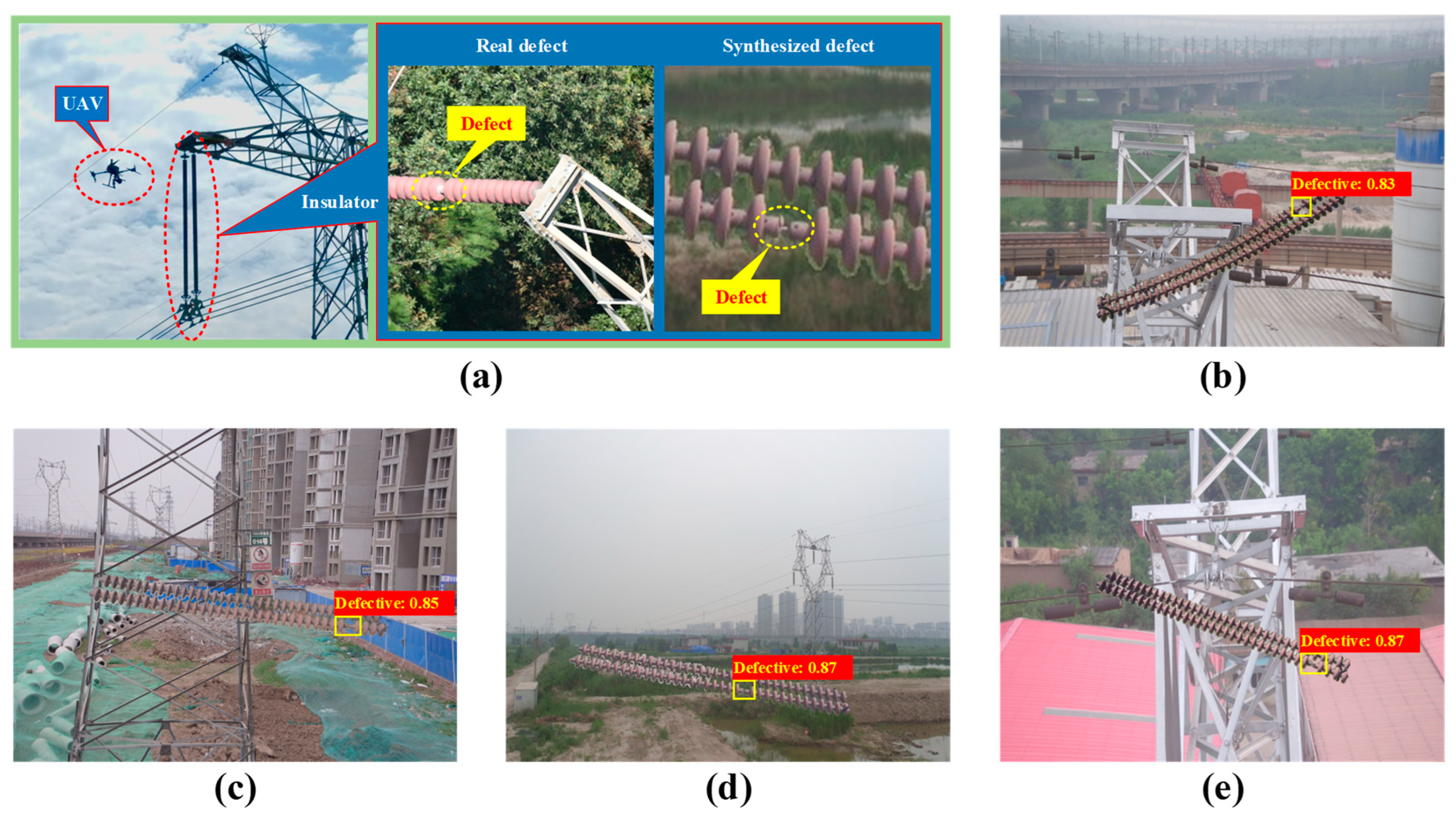
To explore the application potential of our method on objects other than arc magnets, we attempted to use our model for the detection of image-based insulator defects in a high-voltage tower. The data used in this attempt were sourced from the Chinese Power Line Insulator Dataset (CPLID) [42], which provided 600 defect-free insulator images captured by unmanned aerial vehicles (UAVs) and 248 synthetic defective insulator images. All images in this dataset were derived from a synthesis of the ground truth and defective insulators due to the limited number of real defective insulator images. The purpose of this identification was to determine whether the insulator in each image has defects. The same data augmentation was still followed due to the small and unbalanced sample data. The number of images of both defect-free and defective insulators was expanded to 1200, which were also respectively divided into the training set, the validating set, and the testing set according to a ratio of 8:1:1. The model employed wass still derived from a fine-tuned network based on the same pre-trained YOLOv5s and compressed with the help of pruning and distillation. An example of the detection of defective insulators is shown in Figure 10. We found that the defective insulators in the figure could be detected accurately. We chose the original YOLOv5s trained directly with the augmented CPLID data to compare with our model to investigate their performance in detecting defective insulators. As exhibited in

Table 3. Performance comparison of the proposed model and original YOLOv5s in the image-based insulator defect detection.

Model	TNNP (M)	FLOPS (G)	MS (MB)	AITC (mS)	mAP (%)	AD (%)
YOLOv5s	7.064	6.919	27.170	10.046	99.960	98.333
Our model	0.455	0.804	1.906	9.480	99.990	100.000

, compared to the original YOLOv5s, our model reduced TNNP, FLOPS, MS, and AITC by 93.559%, 88.380%, 92.985%, and 5.634%, respectively. This indicates that the complexity and computing power dependence of the model were significantly smaller, implying a faster detection speed and a more convenient deployment. More importantly, mAP increased by 0.03% and $A_D$ was boosted by 1.667% and improved to 100%, enabling the most accurate detection of defective insulators. It follows that there is considerable potential for broader applications given the advantages of our method in compressing models and improving accuracy.

5. Conclusions

This paper proposed a machine-vision method for identifying surface defects on arc magnets. The proposed method combines transfer learning, network pruning, and knowledge distillation for the YOLOv5s model to obtain high recognition accuracy of surface defects while greatly compressing the model size at a slight loss of accuracy, thereby improving the recognition speed. In our work, the type and quantity of the original public image-based dataset of surface defects on arc magnets were appended by us to make the dataset more extensive and representative. To overcome the dependence of model training on massive image-based data of arc magnets, our model was derived from YOLOv5s that had been robustly pre-trained by another publicly available dataset with a large number of different targets other than arc magnets. The transfer-learning mechanism under the frozen and fine-tuned YOLOv5s enabled the target recognition ability obtained by pre-training on the other dataset to be converted into highly accurate surface-defect identification after training based on relatively few image-based arc magnets. The proposed pruning rate, validated by the objective function we designed, achieved an optimal balance between maximizing model compression and minimizing accuracy loss during the network pruning for the transferred YOLOv5s. The unpruned and pruned transferred YOLOv5s were respectively employed as the teacher and student networks for knowledge distillation. A proposed λ weighting factor was introduced into the confidence loss function of knowledge distillation to increase the sensitivity of the student network for extracting and identifying image-based features of surface defects, but such a sensitivity improvement was bound to sacrifice a small amount of recognition accuracy for defect-free arc magnets. The experimental results show that our model is only 1.921 MB in size and can identify any defective arc magnet with 100% accuracy within an average inference time of 9.46 ms. Moreover, the misidentification rate for defect-free arc magnets did not exceed 1%. Considering accuracy, speed, and size together, our model outperforms other conventional lightweight models and is more conducive to high-precision and rapid identification of surface defects on arc magnets under a lightweight model deployment with low computing power. Similar superior performance was also obtained for the detection of insulator defects in a high-voltage tower, for which our model was used to identify image-based insulator data. Given the advantages of our model in compressing models and improving accuracy, more applications based on our method have the potential to be developed.

Even though the identification accuracy of defective arc magnets reached 100%, 1% of defect-free arc magnets still could not be accurately identified. The significant compression of the model size did not result in a substantial reduction of inference time. These phenomena make it necessary to continue improving our method in terms of accuracy and speed, but the corresponding improvements are also limited by the performance of YOLOv5s. Along with developing the YOLO series, we will attempt newer and better YOLO models to update YOLOv5s for the surface-defect identification of arc magnets in future work. Meanwhile, we will continue to explore different model compression methods to achieve faster identification speed.

References

1. Huang, Q.Y.; Xie, L.F.; Yin, G.F.; Ran, M.X.; Liu, X.; Zheng, J. Acoustic signal analysis for detecting defects inside an arc magnet using a combination of variational mode decomposition and beetle antennae search. ISA Trans. 2020, 102, 347–364. [Google Scholar] [CrossRef]
2. Yang, C.L.; Liu, P.Y.; Yin, G.F.; Jiang, H.H.; Li, X.Q. Defect detection in magnetic tile images based on stationary wavelet transform. NDT E. Int. 2016, 83, 78–87. [Google Scholar] [CrossRef]
3. Zhong, Z.Y.; Wang, H.X.; Xiang, D. Small defect detection based on local structure similarity for magnetic tile surface. Electronics 2023, 12, 185. [Google Scholar] [CrossRef]
4. Xie, L.F.; Xiang, X.; Xu, H.N.; Wang, L.; Lin, L.J.; Yin, G.F. FFCNN: A deep neural network for surface defect detection of magnetic tile. IEEE Trans. Ind. Electron. 2020, 68, 3506–3516. [Google Scholar] [CrossRef]
5. Li, X.Q.; Jiang, H.H.; Yin, G.F. Detection of surface crack defects on ferrite magnetic tile. NDT E. Int. 2014, 62, 6–13. [Google Scholar] [CrossRef]
6. Xie, L.F.; Lin, L.J.; Yin, M.; Meng, L.T.; Yin, G.F. A novel surface defect inspection algorithm for magnetic tile. Appl. Surf. Sci. 2016, 375, 118–126. [Google Scholar] [CrossRef]
7. Ling, X.F.; Wu, Y.P.; Ali, R.; Zhu, H.Z. Magnetic tile surface defect detection methodology based on self-attention and self-supervised learning. Comput. Intell. Neurosci. 2022, 2022, 3003810. [Google Scholar] [CrossRef]
8. Yang, C.L.; Liu, P.Y.; Yin, G.F.; Wang, L. Crack detection in magnetic tile images using nonsubsampled shearlet transform and envelope gray level gradient. Opt. Laser Technol. 2017, 90, 7–17. [Google Scholar] [CrossRef]
9. Cui, L.S.; Jiang, X.H.; Xu, M.L.; Li, W.Q.; Lv, P.; Zhou, B. SDDNet: A fast and accurate network for surface defect detection. IEEE Trans. Instrum. Meas. 2021, 70, 1–13. [Google Scholar] [CrossRef]
10. Li, X.Q.; Liu, Z.; Yin, G.F.; Jiang, H.H. Ferrite magnetic tile defects detection based on nonsubsampled contourlet transform and texture feature measurement. Russ. J. Nondestruct. 2020, 56, 386–395. [Google Scholar]
11. Gharsallah, M.B.; Braiek, E.B. Defect identification in magnetic tile images using an improved nonlinear diffusion method. Trans. Inst. Meas. Control 2021, 43, 2413–2424. [Google Scholar] [CrossRef]
12. Li, X.Q.; Liu, Z.; Feng, Z.M.; Zheng, L.; Liu, S. Magnetic tile crack defect detection based on Contourlet transform and singular value decomposition. Nondestruct. Test. Eval. 2022, 37, 820–833. [Google Scholar] [CrossRef]
13. Bhatt, P.M.; Malhan, R.K.; Rajendran, P.; Shah, B.C.; Thakar, S.; Yoon, Y.J.; Gupta, S.K. Image-based surface defect detection using deep learning: A review. J. Comput. Inf. Sci. Eng. 2021, 21, 040801. [Google Scholar] [CrossRef]
14. An, Y.; Lu, Y.N.; Wu, T.R. Segmentation method of magnetic tile surface defects based on deep learning. Int. J. Comput. Commun. 2022, 17, 4502. [Google Scholar] [CrossRef]
15. Hu, C.; Liao, H.W.; Zhou, T.; Zhu, A.J.; Xu, C.P. Online recognition of magnetic tile defects based on UPM-DenseNet. Mater. Today Commun. 2022, 30, 103105. [Google Scholar] [CrossRef]
16. Liu, T.; Ye, W. A semi-supervised learning method for surface defect classification of magnetic tiles. Mach. Vision Appl. 2022, 33, 1–14. [Google Scholar] [CrossRef]
17. Cao, X.C.; Chen, B.Q.; He, W.P. Unsupervised defect segmentation of magnetic tile based on attention enhanced flexible U-Net. IEEE Trans. Instrum. Meas. 2022, 71, 1–10. [Google Scholar] [CrossRef]
18. Liang, W.J.; Sun, Y.R. ELCNN: A Deep Neural Network for Small Object Defect Detection of Magnetic Tile. IEEE Trans. Instrum. Meas. 2022, 71, 1–10. [Google Scholar] [CrossRef]
19. Wu, C.X.; Luo, C.; Xiong, N.X.; Zhang, W.; Kim, T.H. A greedy deep learning method for medical disease analysis. IEEE Access 2018, 6, 20021–20030. [Google Scholar] [CrossRef]
20. Zhang, S.M.; Wu, R.Z.; Xu, K.Y.; Wang, J.M.; Sun, W.W. R-CNN-based ship detection from high resolution remote sensing imagery. Remote Sens. 2019, 11, 631. [Google Scholar] [CrossRef]
21. Li, J.N.; Liang, X.D.; Shen, S.M.; Xu, T.F.; Feng, J.S.; Yan, S.C. Scale-aware fast R-CNN for pedestrian detection. IEEE Trans. Multimed. 2017, 20, 985–996. [Google Scholar] [CrossRef] [Green Version]
22. Lei, X.S.; Sui, Z.H. Intelligent fault detection of high voltage line based on the Faster R-CNN. Measurement 2019, 138, 379–385. [Google Scholar] [CrossRef]
23. Tan, Y.; Cai, R.Y.; Li, J.R.; Chen, P.L.; Wang, M.Z. Automatic detection of sewer defects based on improved you only look once algorithm. Automat. Constr. 2021, 131, 103912. [Google Scholar] [CrossRef]
24. Yi, J.R.; Wu, P.X.; Metaxas, D.N. ASSD: Attentive single shot multibox detector. Comput. Vis. Image Underst. 2019, 189, 102827. [Google Scholar] [CrossRef]
25. Wang, D.D.; He, D.J. Channel pruned YOLO V5s-based deep learning approach for rapid and accurate apple fruitlet detection before fruit thinning. Biosyst. Eng. 2021, 210, 271–281. [Google Scholar] [CrossRef]
26. Xu, Z.B.; Huang, X.P.; Huang, Y.; Sun, H.B.; Wan, F.X. A real-time zanthoxylum target detection method for an intelligent picking robot under a complex background, based on an improved YOLOv5s architecture. Sensors 2022, 22, 682. [Google Scholar] [CrossRef] [PubMed]
27. Zhao, S.Z.; Kang, F.; Li, J.J. Concrete dam damage detection and localisation based on YOLOv5s-HSC and photogrammetric 3D reconstruction. Autom. Constr. 2022, 143, 104555. [Google Scholar] [CrossRef]
28. Shell, J.; Coupland, S. Fuzzy transfer learning: Methodology and application. Inform. Sci. 2015, 293, 59–79. [Google Scholar] [CrossRef]
29. Saber, A.; Sakr, M.; Abo-Seida, O.M.; Keshk, A.; Chen, H.L. A novel deep-learning model for automatic detection and classification of breast cancer using the transfer-learning technique. IEEE Access 2021, 9, 71194–71209. [Google Scholar] [CrossRef]
30. Ali, M.S.; Miah, M.S.; Haque, J.; Rahman, M.M.; Islam, M.K. An enhanced technique of skin cancer classification using deep convolutional neural network with transfer learning models. Mach. Lear. Appl. 2021, 5, 100036. [Google Scholar] [CrossRef]
31. Wang, Z.Y.; Li, F.; Shi, G.; Xie, X.M.; Wang, F.Y. Network pruning using sparse learning and genetic algorithm. Neurocomputing 2020, 404, 247–256. [Google Scholar] [CrossRef]
32. Wang, L.; Yoon, K.J. Knowledge distillation and student-teacher learning for visual intelligence: A review and new outlooks. IEEE Trans. Pattern. Anal. 2021, 44, 3048–3068. [Google Scholar] [CrossRef] [PubMed]
33. Jiang, Y.; Wang, S.Q.; Valls, V.; Ko, B.J.; Lee, W.H.; Leung, K.K.; Tassiulas, L. Model pruning enables efficient federated learning on edge devices. IEEE Trans. Neural Netw. Learn. 2022, 1–13. [Google Scholar] [CrossRef] [PubMed]
34. Xu, Q.; Chen, Z.H.; Wu, K.Y.; Wang, C.; Wu, M.; Li, X.L. KDnet-RUL: A knowledge distillation framework to compress deep neural networks for machine remaining useful life prediction. IEEE Trans. Ind. Electron. 2021, 69, 2022–2032. [Google Scholar] [CrossRef]
35. Ying, Z.P.; Lin, Z.T.; Wu, Z.Y.; Liang, K.; Hu, X.D. A modified-YOLOv5s model for detection of wire braided hose defects. Measurement 2022, 190, 110683. [Google Scholar] [CrossRef]
36. Zhuang, F.Z.; Qi, Z.Y.; Duan, K.Y.; Xi, D.B.; Zhu, Y.C.; Zhu, H.S.; Xiong, H.; He, Q. A comprehensive survey on transfer learning. Proc. IEEE 2020, 109, 43–76. [Google Scholar] [CrossRef]
37. Liang, T.L.; Glossner, J.; Wang, L.; Shi, S.B.; Zhang, X.T. Pruning and quantization for deep neural network acceleration: A survey. Neurocomputing 2021, 461, 370–403. [Google Scholar] [CrossRef]
38. Gou, J.P.; Yu, B.S.; Maybank, S.J.; Tao, D.C. Knowledge distillation: A survey. INT. J. Comput. Vis. 2021, 129, 1789–1819. [Google Scholar] [CrossRef]
39. Huang, Y.B.; Qiu, C.Y.; Yuan, K. Surface defect saliency of magnetic tile. Vis. Comput. 2020, 36, 85–96. [Google Scholar] [CrossRef]
40. Yan, B.; Fan, P.; Lei, X.Y.; Liu, Z.J.; Yang, F.Z. A real-time apple targets detection method for picking robot based on improved YOLOv5. Remote Sens. 2021, 13, 1619. [Google Scholar] [CrossRef]
41. Basheer Ahmed, M.I.; Zaghdoud, R.; Ahmed, M.S.; Sendi, R.; Alsharif, S.; Alabdulkarim, J.; Albin Saad, B.A.; Alsabt, R.; Rahman, A.; Krishnasamy, G. A real-time computer vision based approach to detection and classification of traffic incidents. Big Data Cogn. Comput. 2023, 7, 22. [Google Scholar] [CrossRef]
42. Tao, X.; Zhang, D.P.; Wang, Z.H.; Liu, X.L.; Zhang, H.Y.; Xu, D. Detection of power line insulator defects using aerial images analyzed with convolutional neural networks. IEEE Trans. Syst. Man Cybern. Syst. 2018, 50, 1486–1498. [Google Scholar] [CrossRef]
Figure 1. The YOLOv5s structure.
Applsci 13 02078 g001
Figure 2. Proposed framework for identifying arc magnet surface defects.
Applsci 13 02078 g002
Figure 3. The experimental rig designed to identify the surface defects on arc magnets: (a) the three-dimensional diagram; (b) partial actual details of the individual identification of each arc magnet; (c) partial actual details of the simultaneous identification of multiple arc magnets.
Applsci 13 02078 g003
Figure 4. The appearance of experimental samples and the data augmentation of their images: (a) the appearance of experimental samples; (b) the data augmentation.
Applsci 13 02078 g004
Figure 5. Transfer learning effects: (a) the mAP@0.5 result for different combinations of freezing and fine-tuning; (b) the training loss result for different combinations of freezing and fine-tuning; (c) the visualization difference of the output of the last CSP1-X in the backbone network between the un-frozen and un-tuned YOLOv5s model and the transferred YOLOv5s model; (d) results of the surface defect identification based on the transferred and un-transferred YOLOv5s.
Applsci 13 02078 g005
Figure 6. Results of network pruning in the transferred model: (a) our network pruning strategy; (b) the visualization for the initial output of the specific layer in our model; (c) the visualization for the channel removal in the specific layer under descending L 2 norm value; (d) influence on network pruning on the model performance; (e) the impact of different pruning rates on F x in the validating set; (f) changes in the number of channels before and after pruning.
Applsci 13 02078 g006
Figure 7. Results of the knowledge distillation for the student network: (a) the contribution of the introduced weight factor λ to the accuracy improvement; (b) the mAP and loss of student network during the training process; (c) the output visualization of the specific layer in the networks before and after knowledge distillation.
Applsci 13 02078 g007
Figure 8. Identification results for the testing set: (a) confusion matrix of identification results; (b) visualization of identification results.
Applsci 13 02078 g008
Figure 9. Performance of different models for identifying surface defects.
Applsci 13 02078 g009
Figure 10. An example of the detection of defective insulators using our model: (a) the schematic of the insulator defect detection and its images; (be) the identification effect of different defective insulators synthesized with ground-truth images.
Applsci 13 02078 g010